A Novel Sliding Mode Control Scheme for a PMSG-Based Variable Speed Wind Energy Conversion System


1
University Center for Exact Sciences and Engineering, University of de Guadalajara, Guadalajara 44430, Mexico
2
Advanced Studies and Research Center (CINVESTAV), National Polytechnic Institute (IPN), Guadalajara Campus, Zapopan 45015, Mexico
3
CONACYT–Advanced Studies and Research Center (CINVESTAV), National Polytechnic Institute (IPN), Guadalajara Campus, Zapopan 45015, Mexico
*
Author to whom correspondence should be addressed.
†
These authors contributed equally to this work.
Energies 2017, 10(10), 1476; https://doi.org/10.3390/en10101476
Submission received: 5 August 2017
/
Revised: 10 September 2017
/
Accepted: 12 September 2017
/
Published: 24 September 2017
(This article belongs to the Special Issue Wind Generators Modelling and Control)
Abstract
:This work proposes a novel control scheme for a variable speed wind turbine system based on the permanent magnet synchronous generator. Regions II and III for a wind speed profile are considered, hence the control is designed for maximizing the generated power from the wind turbine when the wind speed is below the nominal wind speed, and to saturate the generated power when the wind speed is above its nominal value in order to avoid damage to the system. Based on nonlinear models, the control scheme is also designed for introducing robustness to the closed-loop system. The pitch angle reference signal is also designed based on a mathematical model of the system, yielding in that way to a great performance of the wind turbine as predicted by the numeric simulations.
1. Introduction
In recent years, the demand for electrical energy has been an important aspect in a global context, where fossil fuels are the main sources for the generation of electrical energy. These sources of energy have significant disadvantages since their use produces the emission of gases that pollute the atmosphere, and in addition to that, the reserves are beginning to be depleted [1]. For these reasons, renewable energy is playing a decisive role in the generation of electricity [2]. The renewable energies include hydropower, wind, solar, geothermal, marine energy, biomass and biofuels. Nowadays, there is a significant increase in the exploitation of wind energy, and as consequence, this has become an interesting research area for the last three decades [3,4].
One of the basic constituents of a wind speed conversion system is the wind turbine, which is a set mainly formed by the blades and the electric generator. As far as the electric generator is concerned, it is the one that is responsible for converting the mechanical energy (transmitted from the blades) into electrical energy. At present, there are mainly two types of electric generators: the induction generator and the synchronous generator. In particular, the permanent magnet synchronous generator (PMSG) is gaining popularity with respect to the induction generator (double-fed and squirrel-cage) [5], due to the fact that a synchronous machine with permanent magnets does not have rotor winding so its lost power is lower, and, as a consequence, its efficiency is greater than that of an induction machine [6]. Another aspect to highlight is that the volume and weight of a synchronous machine with permanent magnets are much smaller than those of an induction machine.
Regarding the control of synchronous generators with permanent magnets, it has become a challenge for electrical engineers since it is a nonlinear coupled system with uncertain parameters [4]. Nowadays, the related control problems to a wind conversion system are to control such systems under an unknown fluctuating wind source. This fact yields to four operational regions for variable speed turbines as described in [7]. Region I is characterized by a wind speed delimited by 0 m/s and by the cut-in value. In this region, the generator is disconnected from the grid. Region II operates from the cut-in value to the nominal wind speed, where a control algorithm is designed for maximizing the captured wind energy. In this region, the pitch angle is controlled to the set-point value of . Region III operates above the nominal wind speed bounded by the cut-out value. In this region, the pitch angle is controlled for the tracking of a desired pitch angle signal that must be generated in such a way that guarantees the operation of the wind turbine as in nominal wind conditions. Region IV is characterized by a wind speed that exceeds the cut-out value, in this case, the generator is disconnected and the turbine is stopped.
Some researchers have focused their attention in the designing of control algorithms for Region II and/or Region III. For example, in [7], two control algorithms are designed based on a bumpless transfer technique for switching between Region II and III, which avoids the bumps at the switching instant of controllers. Despite the control technique employed, the separated controllers are simple PID controllers where the variation of plant parameters is not considered; moreover, the generation of the reference signal for the pitch angle () is not described. In the work presented in [8], a sliding mode controller based on the backstepping tehcnique is designed just for the mechanical part of the wind turbine where the design of is not specified. The work [9] presents a controller for the maximum power point tracking (MPPT) by means of a lookup table. The work [10] is devoted to the pitch angle control design, where is calculated from a pitch angle versus wind speed curve obtained by means of the boundary element method for a given turbine. In the work [11], a single controller (based on the sliding mode technique) for the generator along with a single pitch angle controller are proposed for Regions II and III, where the pitch angle command signal is generated without .
Despite the efforts made by researchers for controlling variable speed wind energy systems, there is a need for designing suitable controllers for Regions II and III that can be robust to unknown bounded perturbations (wind fluctuations) and plant parameters’ variations, along with a clear design of both and the corresponding pitch angle controller.
Hence, in this work, we are compelled with the design of two control schemes for Regions II and III. For Region II, we propose a controller based on the sliding mode technique for the regulation of an optimal rotor speed based on MPPT, where the super twisting algorithm (STA) is used since it alleviates the well known chattering problem [12,13]. In this region, is fixed to zero. For Region III, a controller based on the sliding mode technique is designed for the regulation of the rotor speed to the optimal speed, where the pitch angle () is considered as pseudo-control variable that becomes in ; then, considering the actuator dynamics for the blades, a controller based on a PI strategy is designed for the tracking of . Finally, a STA is proposed for regulating the electrical torque of the generator for the tracking of the sum of the mechanical and frictional torques in order to prevent the instability of the mechanical dynamics of the generator.
The organization of the rest of the work is as follows. Section 2 describes the dynamics of the wind turbine, generator, and the pitch angle actuator. In Section 3, the control strategies are designed for the variable speed wind energy conversion system, and the simulation results are presented in Section 4. Final comments are presented in Section 5.
2. System Modeling
This section deals with the mathematical modeling of the wind turbine, the synchronous generator with permanent magnets mounted on the surface, and the pitch angle actuator.
2.1. Wind Turbine Model
The aerodynamic power can be expressed as follows [14,15]:
where is the air density, is the power performance coefficient, is the wind speed upstream of the rotor and A is the area swept by the rotor. The variable is the corresponding angle for the blade pitch (in degree), and the tip-speed ratio is represented by and it is expressed by:
with as the angular rotor speed, and R being the radius of the blade. The power coefficient as a function of and is defined as:
Finally, the wind turbine mechanical torque output is given as:
2.2. Generator Model
Assuming a mechanical transmission with unitary conversion factor, the surface mounted PMSG dynamics are presented with respect to the reference frame fixed to the rotor [16]:
with L as the stator inductance, is the stator resistance, is the permanent magnetic flux linkage, is the number of pole pairs, J is the moment of inertia of the system, and F is the viscous friction coefficient. The variables are as the electromagnetic torque, is the mechanical torque developed by the turbine, and are the stator currents, and are the stator voltages, and , and are unknown bounded perturbations due to plant parameter variations.
2.3. Pitch Angle Actuator Model
The actuator for the pitch consists of an electromechanical and/or an electrohydraulic system. The mathematical model for the actuator relates the output of the pitch controller (pitch demand represented by ) and the real pitch angle . For a variable-speed wind turbine, an electromechnical actuator is commonly used for regulating the angle of the pitch, so the power coefficient is decreased and the power lies at its rated value [17]. The actuator dynamics can be approximated as a first order system:
where is the time constant of the actuator [18].
3. Development of the Control Strategy
3.1. Maximum Power Point
For the maximum power point (MPP), the speed of the turbine must be determined for a given wind velocity as in [19]. For that, the turbine speed derivative of Equation (1) is taken
with
Under condition one can determine the value for the turbine speed that yields to a MPP:
Since, for Region II, we have that , the optimal turbine speed is defined as follows:
where is the optimal tip-speed ratio. From Equation (5), one can define the nominal turbine speed as:
with as the nominal wind velocity. The maximum power of the turbine system is given as:
where , and the nominal power and torque generated by the turbine are:
3.2. Rotor Speed Control Design for Region II
In order to achieve the MPPT below the nominal wind speed, one proposes the tracking error as follows:
The dynamics of the tracking error result as:
where is considered as a pseudo-control input and can be proposed as a desired signal of the following form:
with as a sigmoidal function that is defined as follows:
Sigmoidal functions approximate the discontinuous sign function with a smooth function, permitting in that way to continue with the control design procedure. Hence, one can write , with , with [20]. Thus, sigmoidal functions provide robustness to the closed-loop system in the presence of unknown bounded and matched perturbations. Continuing with the control design, one defines the tracking errors for the stator currents:
where usually is set to zero for maximizing the torque [12]. The dynamics for tracking error result as follows:
Then, we propose as a sliding mode controller based on the equivalent control method and the STA
with and as positive design gains, and as the equivalent controller that results from the nominal equation (without perturbation term) as follows:
Now, we continue with the dynamics of :
where is proposed in a similar fashion to :
with and as positive design gains, and as the equivalent controller calculated from
The new variables , , and define a diffeomorphism that yields system (3) to the following form:
It has already been shown in [21] that, with appropriate gain values, the STA will ensure that and reach zero in finite-time. Then, when the sliding mode takes place, i.e., , the resulting sliding mode dynamics is as follows:
3.3. Pitch Angle and Electrical Torque Controller Designs for Region III
When the wind speed exceeds its nominal value, the power generated by the turbine exceeds its nominal value, so the wind turbine can be damaged. Hence, we propose a pitch angle controller where the reference signal for the pitch angle is obtained by controlling the rotor speed in a master–slave control scheme. By controlling the pitch angle, the turbine variables as the power, the torque and the speed will reach its corresponding nominal values, and the generator is controlled for guaranteeing that its electrical torque can track the sum of the mechanical and frictional torques in order to avoid the instability of the mechanical dynamics of the generator.
3.3.1. Pitch Angle Control Design
Based on a master–slave control scheme, we first propose the tracking error for the rotor speed as . By using Equation (2), the corresponding dynamics for are as follows:
where is considered as a pseudo control input, and it is determined as a reference signal () of the following form:
where is the sigmoidal function already introduced in Section 3.2, as a positive design gain, and will be defined in the following lines. It is worth noting that the reference signal () in Equation (19) depends on , where this variable is an estimate of . If this estimate is not used, then an algebraic loop is created. The estimation is obtained by using a sliding mode differentiator [22]:
with , , and as positive design gains, the estimate of is , and the estimate of its time derivative is . This approach is useful when the control variable depends on itself and/or its time derivative as already shown in [23,24].
Now, we define the tracking error for the pitch angle as , and, with the help of Equation (4), the corresponding dynamics for are as follows:
Now, is proposed as a PI controller:
with as the time derivative of the estimated reference signal for the pitch angle and it is generated from the the robust differentiator (20). The new variables and define a new system, that, when closed-loop with Equation (21) yields to the following form:
where is a nonlinear function that satisfies .
According to [22], if it is considered that the signal is bounded and free of noise, then, the robust differentiator (20) guarantees finite-time convergence of the relations: and . Hence, system (22) reduces to:
3.3.2. Electrical Torque Control Design
Let us define the tracking errors for the electrical torque and the direct current component as follows:
where is set to zero. Their corresponding dynamics are of the following form:
The control input signals and are proposed with the equivalent control method and the STA:
with , , , as positive design gains, and and as a solution of the nominal equations and , respectively. As already mentioned, in the work presented in [21], it was shown that, with suitable gain values, the STA will ensure that and reach zero in finite-time.
A block diagram of the proposed solution is shown in Figure 1.
4. Simulation Results
Simulations were carried out for the performance verification of the closed-loop system. We consider a wind turbine system with nominal parameters as shown in Table 1. The control gains have been chosen as in Table 2.
The robustness of the closed-loop system is verified with plant parameters’ variations; for that, we have considered an increment of with respect to the corresponding nominal values for J and . The behaviour of the wind speed is presented in Figure 2, which is varying above and below the nominal wind speed at 12 m/s. The crossing points at the nominal wind speed are located at 0.45, 2.66 and 3.81 s approximately.
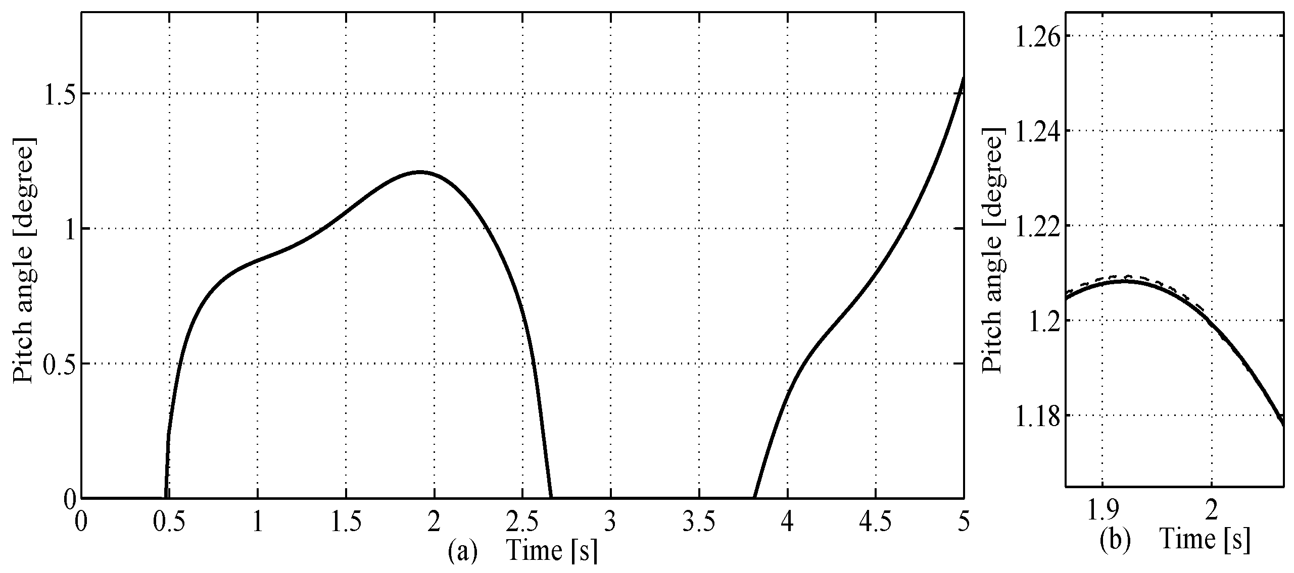
Figure 3 shows the pitch angle. One can note that, when the wind speed is below the nominal value, the pitch angle is zero, and, when the wind speed is above the nominal value, the pitch angle is greater than zero in order to compensate the extra wind power.
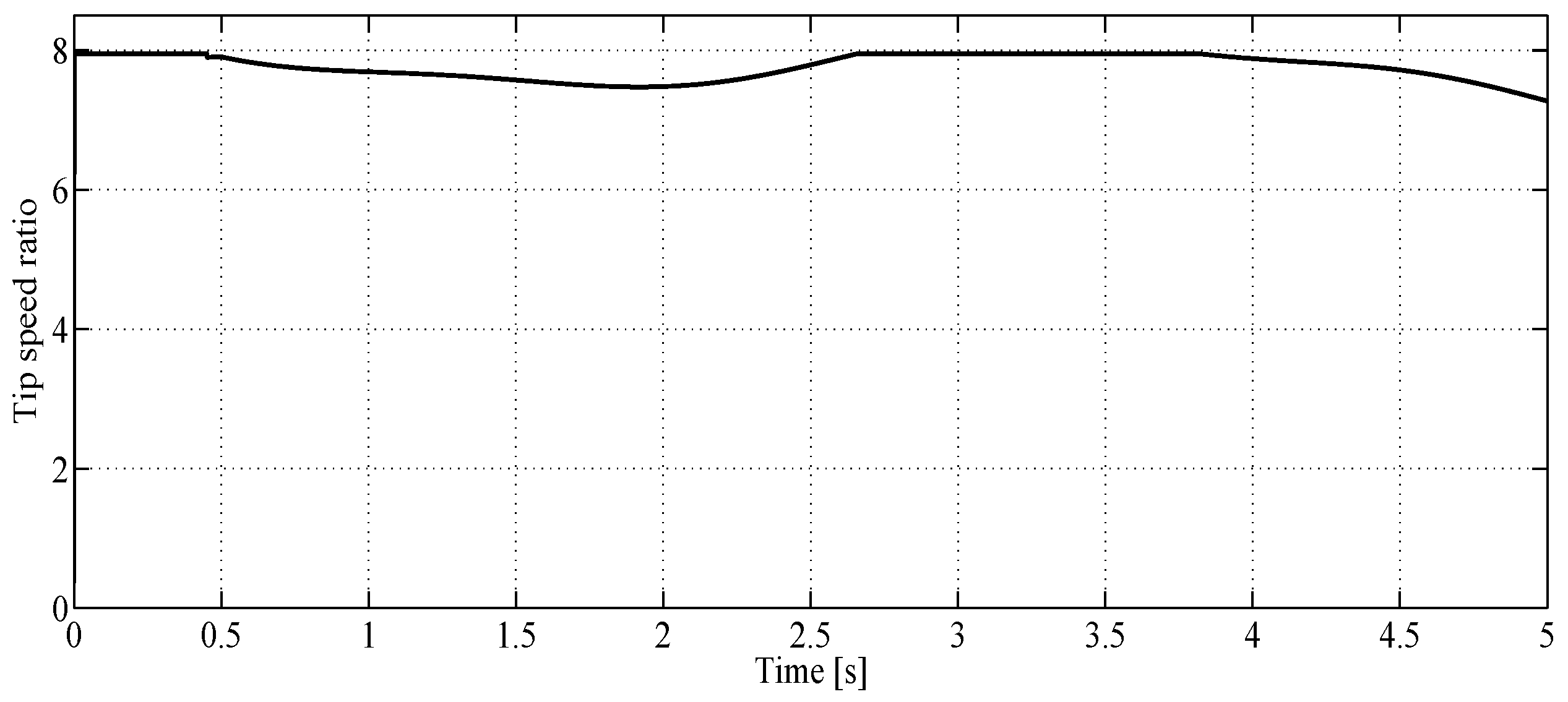
The power performance coefficient and the tip speed ratio are shown in Figure 4 and Figure 5, respectively. One can observe in and that, when the speed of the wind is underneath its nominal value, they are fixed at the optimal values and , respectively. In the case that the speed of the wind is above its nominal value, both signals are decreasing their corresponding values.
Figure 6 shows the behaviour of the optimal and real rotor speed of the generator. The first one varies up to a maximum value of 2.38 rad/s when the speed of the wind is above its nominal value.
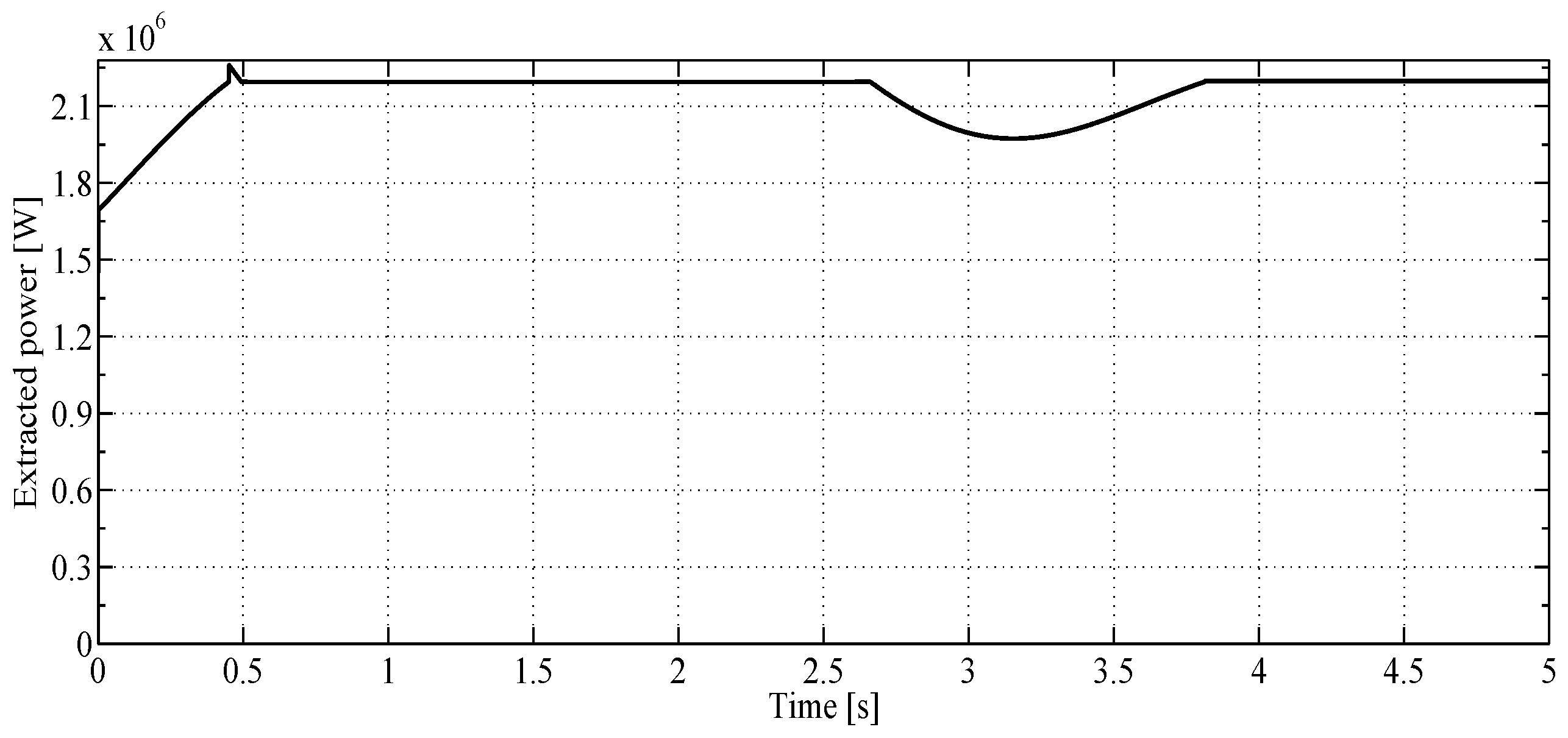
The generated power is shown in Figure 7. One can note that the MPPT is achieved satisfactorily. The power is saturated at the nominal value of 2.195 MW thanks to the pitch angle and torque controllers.
5. Conclusions
Renewable energies are playing an important role for the electrical energy generation, where the wind energy exploitation is a current research area. Generators such as the PMSG are gaining popularity with respect to the induction generator due to fact that PMSG are characterized by a lower lost power, volume and weight. Current research on the control of a wind turbine system based on PMSG fail when simplified mathematical models are considered in the design of controllers for Regions II and III, and for the design of the reference signal for the pitch angle. Hence, in this work, the proposed controllers for the wind turbine system in Regions II and III are well designed, since they are based on the characteristics of such regions, on nonlinear models and a novel control algorithm as the STA. In addition, the reference signal for the pitch angle is also well designed since it is based on the mathematical model of the system, and, as a consequence of this, the wind turbine operates at its nominal point when wind speed variations are greater than its nominal value. Moreover, thanks to the introduction of sigmoidal functions, the proposed controllers are robust against plant parameter variations, as just demonstrated with the numeric simulations. Some issues remain such as the control design for the grid side and the evaluation of the proposed algorithm with a prototype.
Acknowledgments
Florentino Chavira is grateful for the grant provided by the National Council of Science and Technology (CONACYT) México.
Author Contributions
The authors contributed equally to this work.
Conflicts of Interest
The authors declare no conflict of interest.
References
- Shafiee, S.; Topal, E. When will fossil fuel reserves be diminished? Energy Policy 2009, 37, 181–189. [Google Scholar] [CrossRef]
- Ahmad, A.; Khan, A.; Javaid, N.; Hussain, H.M.; Abdul, W.; Almogren, A.; Alamri, A.; Azim Niaz, I. An optimized home energy management system with integrated renewable energy and storage resources. Energies 2017, 10, 549. [Google Scholar] [CrossRef]
- Shi, J.; Wang, L.; Wang, Y.; Zhang, J. Generalized energy flow analysis considering electricity gas and heat subsystems in local-area energy systems integration. Energies 2017, 10, 514. [Google Scholar] [CrossRef]
- Sahin, P.; Resmi, R.; Vanitha, V. PMSG based standalone wind electric conversion system with MPPT. In Proceedings of the 2016 International Conference on Emerging Technological Trends (ICETT), Kollam, India, 21–22 October 2016; pp. 1–5. [Google Scholar]
- Li, S.; Li, J. Output predictor-based active disturbance rejection control for a wind energy conversion system with PMSG. IEEE Access 2017, 5, 5205–5214. [Google Scholar] [CrossRef]
- Housseini, B.; Okou, A.F.; Beguenane, R. Performance comparison of variable speed PMSG-based wind energy conversion system control algorithms. In Proceedings of the 2017 Twelfth International Conference on Ecological Vehicles and Renewable Energies (EVER), Monte Carlo, Monaco, 11–13 April 2017; pp. 1–10. [Google Scholar]
- Chen, Q.; Li, Y.; Seem, J.E. Bumpless transfer-based inter-region controller switching of wind turbines for reducing power and load fluctuation. IEEE Trans. Sustain. Energy 2016, 7, 23–31. [Google Scholar] [CrossRef]
- Rajendran, S.; Jena, D. Backstepping sliding mode control for variable speed wind turbine. In Proceedings of the 2014 Annual IEEE India Conference (INDICON), Pune, India, 11–13 December 2014; pp. 1–6. [Google Scholar]
- Mohammadi, E.; Fadaeinedjad, R.; Shariatpanah, H.; Moschopoulos, G. Performance evaluation of yaw and stall control for small-scale variable speed wind turbines. In Proceedings of the 30th IEEE Canadian Conference on Electrical and Computer Engineering (CCECE), Windsor, ON, Canada, 30 April–3 May 2017; pp. 1–4. [Google Scholar]
- Abir, A.; Mehdi, D.; Lassaad, S. Pitch angle control of the variable speed wind turbine. In Proceedings of the 17th International Conference on Sciences and Techniques of Automatic Control and Computer Engineering (STA), Sousse, Tunisia, 19–21 December 2016; pp. 582–587. [Google Scholar]
- Errami, Y.; Ouassaid, M.; Cherkaoui, M.; Maaroufi, M. Sliding mode control scheme of variable speed wind energy conversion system based on the PMSG for utility network connection. In Advances and Applications in Sliding Mode Control Systems; Azar, A.T., Zhu, Q., Eds.; Springer International Publishing: Cham, Germany, 2015; pp. 167–200. [Google Scholar]
- Utkin, V.; Guldner, J.; Shi, J. Sliding Mode Control in Electro-Mechanical Systems, 2nd ed.; Automation and Control Engineering; CRC Press: Boca Raton, FL, USA, 2009. [Google Scholar]
- Rivera, J.; Garcia, L.; Mora, C.; Raygoza, J.J.; Ortega, S. Super-twisting sliding mode in motion control systems. In Sliding Mode Control; InTech: Rijeka, Croatia, 2011. [Google Scholar]
- Ackermann, T. Wind Power in Power Systems; Wiley: Hoboken, NJ, USA, 2012. [Google Scholar]
- Freris, L. Wind Energy Conversion Systems; Prentice Hall: Upper Saddle River, NJ, USA, 1990. [Google Scholar]
- Wu, B.; Lang, Y.; Zargari, N.; Kouro, S. Power Conversion and Control of Wind Energy Systems; IEEE Press Series on Power Engineering; Wiley: Hoboken, NJ, USA, 2011. [Google Scholar]
- Zhang, J.; Cheng, M.; Chen, Z.; Fu, X. Pitch angle control for variable speed wind turbines. In Proceedings of the 2008 Third International Conference on Electric Utility Deregulation and Restructuring and Power Technologies, Nanjing, China, 6–9 April 2008; pp. 2691–2696. [Google Scholar]
- Eisenhut, C.; Krug, F.; Schram, C.; Klockl, B. Wind-turbine model for system simulations near cut-in wind speed. IEEE Trans. Energy Convers. 2007, 22, 414–420. [Google Scholar] [CrossRef]
- Agarwal, V.; Aggarwal, R.K.; Patidar, P.; Patki, C. A novel scheme for rapid tracking of maximum power point in wind energy generation systems. IEEE Trans. Energy Convers. 2010, 25, 228–236. [Google Scholar] [CrossRef]
- Gennaro, S.D.; Domínguez, J.R.; Meza, M.A. Sensorless high order sliding mode control of induction motors with core loss. IEEE Trans. Ind. Electron. 2014, 61, 2678–2689. [Google Scholar] [CrossRef]
- Chalanga, A.; Kamal, S.; Fridman, L.M.; Bandyopadhyay, B.; Moreno, J.A. Implementation of super-twisting control: Super-twisting and higher order sliding-mode observer-based approaches. IEEE Trans. Ind. Electron. 2016, 63, 3677–3685. [Google Scholar] [CrossRef]
- Levant, A. Robust exact differentiation via sliding mode technique. Automatica 1998, 34, 379–384. [Google Scholar] [CrossRef]
- Espinoza-Jurado, J.; Dávila, E.; Rivera, J.; Raygoza-Panduro, J.J.; Ortega, S. Robust control of the air to fuel ratio in spark ignition engines with delayed measurements from a UEGO sensor. Math. Probl. Eng. 2015, 2015, 1–13. [Google Scholar] [CrossRef]
- Castillo-Toledo, B.; Cuevas, A.L. Tracking through singularities using a robust differentiator. In Proceedings of the 2009 6th International Conference on Electrical Engineering, Computing Science and Automatic Control (CCE), Toluca, Mexico, 10–13 January 2009; pp. 1–5. [Google Scholar]
Figure 1.
Block diagram of the proposed control strategy, where is fixed at zero, and corresponds to Equation (19).
Figure 1.
Block diagram of the proposed control strategy, where is fixed at zero, and corresponds to Equation (19).
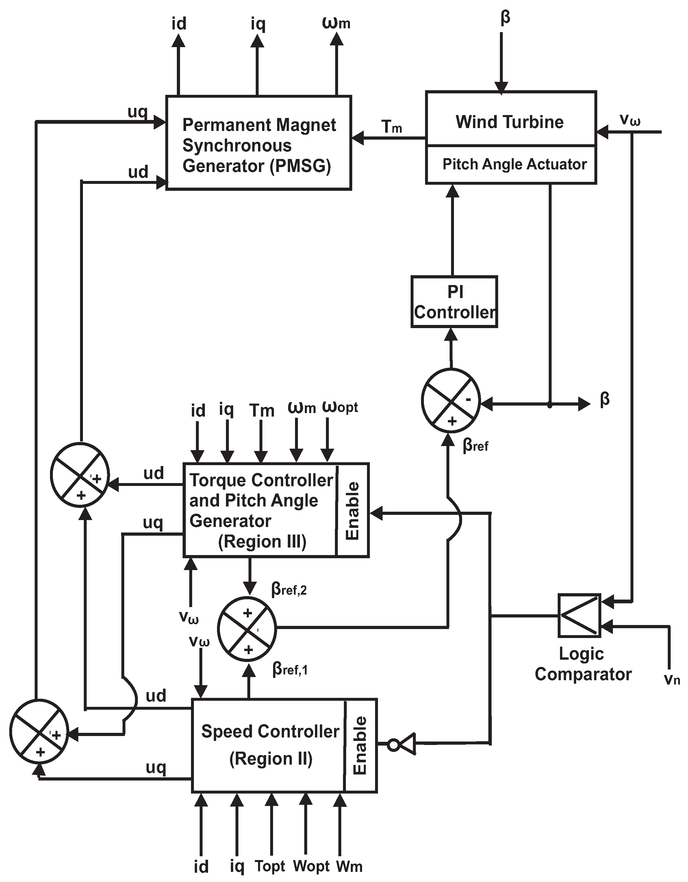
Figure 2.
Wind speed profile.
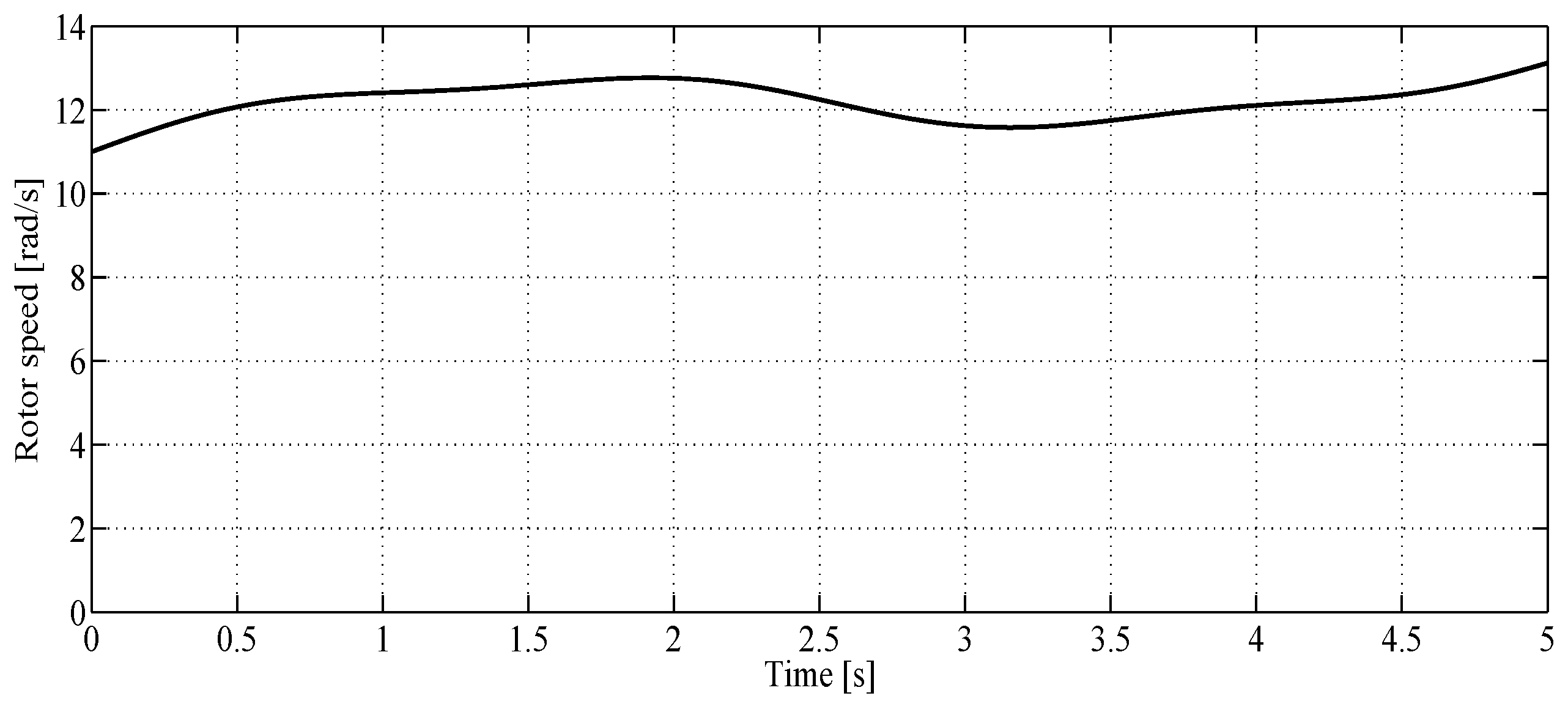
Figure 3.
(a) vs. ; dashed , solid ; (b) zoom of the figure on the left.

Figure 4.
Power performance coefficient, .

Figure 5.
Tip speed ratio, .

Figure 6.
(a) vs ; dashed , solid ; (b) zoom of the figure on the left.
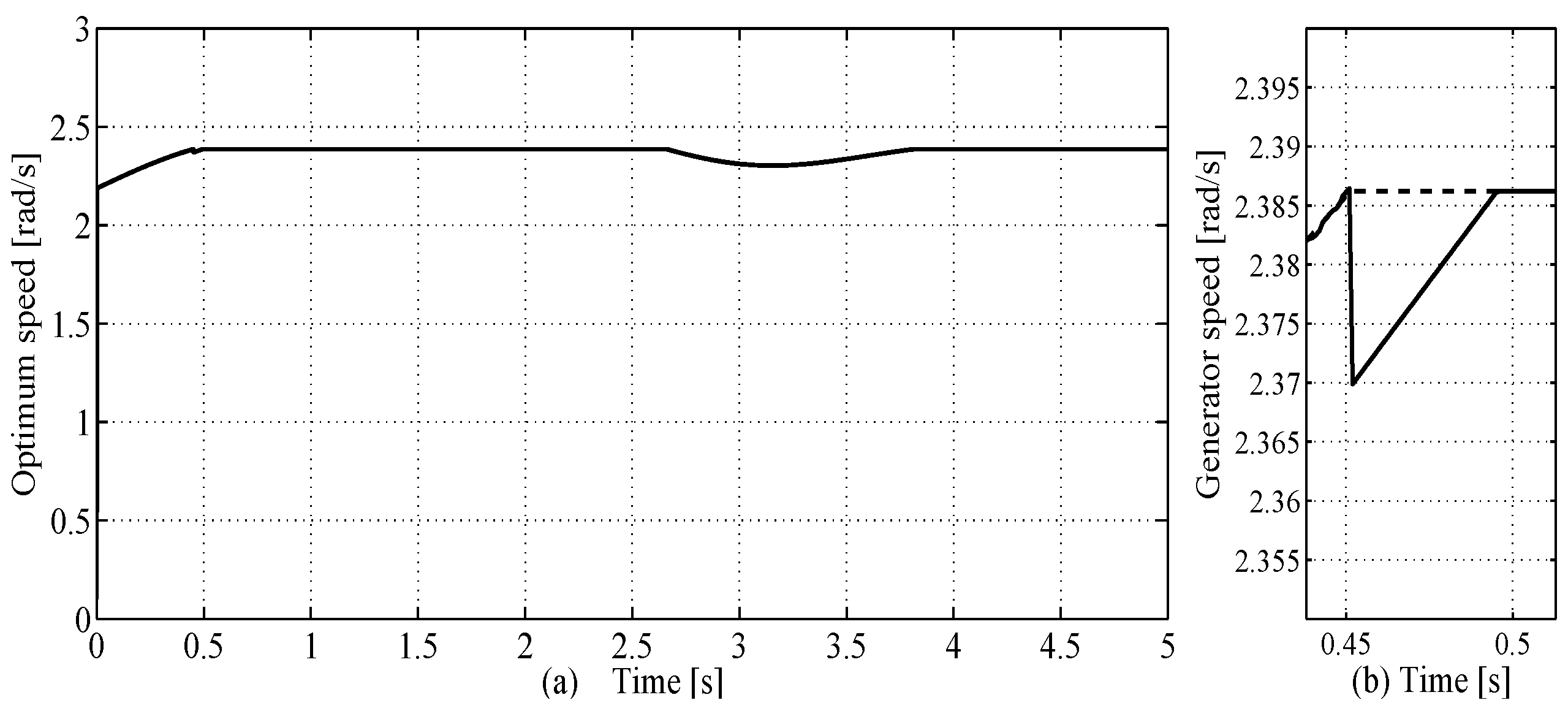
Figure 7.
Generated turbine power, .

Table 1.
Plant parameters for the synchronous generator and wind turbine.
| Parameter | Value | Parameter | Value |
|---|---|---|---|
| 2.195 MW | 0.0008 | ||
| 1.23 kg/m3 | L | 0.61 H | |
| A | 5026.54 m2 | 3.86 Wb | |
| 12 m/s | 60 | ||
| 2.3862 rad/s | J | 10 kg m2 | |
| 1 s | − | − |
Table 2.
Speed controller gains.
| Gains | Value | Gains | Value | Gains | Value |
|---|---|---|---|---|---|
| 135 | 3p /(1000L) | 600 | |||
| 150 | 20/L | 10 | |||
| 300 | 10 | 1 | |||
| 500,000 | 500 | 150 | |||
| 20 | 200 | 20 | |||
| 0.001 | 0.001 | − | − |
© 2017 by the authors. Licensee MDPI, Basel, Switzerland. This article is an open access article distributed under the terms and conditions of the Creative Commons Attribution (CC BY) license (http://creativecommons.org/licenses/by/4.0/).
Share and Cite
MDPI and ACS Style
Chavira, F.; Ortega-Cisneros, S.; Rivera, J. A Novel Sliding Mode Control Scheme for a PMSG-Based Variable Speed Wind Energy Conversion System. Energies 2017, 10, 1476. https://doi.org/10.3390/en10101476
AMA Style
Chavira F, Ortega-Cisneros S, Rivera J. A Novel Sliding Mode Control Scheme for a PMSG-Based Variable Speed Wind Energy Conversion System. Energies. 2017; 10(10):1476. https://doi.org/10.3390/en10101476
Chicago/Turabian StyleChavira, Florentino, S. Ortega-Cisneros, and Jorge Rivera. 2017. "A Novel Sliding Mode Control Scheme for a PMSG-Based Variable Speed Wind Energy Conversion System" Energies 10, no. 10: 1476. https://doi.org/10.3390/en10101476
Note that from the first issue of 2016, this journal uses article numbers instead of page numbers. See further details here.