Optimal Allocation of Photovoltaic Systems and Energy Storage Systems based on Vulnerability Analysis


1
Graduate School of Science and Technology, Keio University, Yokohama 223-0061, Japan
2
Faculty of Science and Technology, Keio University, Yokohama 223-0061, Japan
3
Japan Science and Technology Agency (JST), CREST, Kawaguchi 332-0012, Japan
*
Author to whom correspondence should be addressed.
Energies 2017, 10(10), 1477; https://doi.org/10.3390/en10101477
Submission received: 22 August 2017
/
Revised: 15 September 2017
/
Accepted: 20 September 2017
/
Published: 24 September 2017
(This article belongs to the Special Issue Resilience of Energy Systems 2017)
Abstract
:There is a growing need to connect renewable energy systems (REs), such as photovoltaic systems (PVs), to the power grid for solving environmental problems such as global warming. However, an electricity grid with RE is vulnerable to problems of power shortage and surplus owing to the uncertainty of RE outputs and grid failures. Energy storage systems (ESSs) can be used to solve supply reliability problems, but their installation should be minimized considering their high costs. This study proposes a method to optimize the allocations of PVs and ESSs based on vulnerability analysis, and utilizes our proposed concept of “slow” and “fast” ESSs, which can reflect the influences of both uncertainties: PV outputs and grid failures. Accordingly, this paper demonstrates an optimal allocation of PVs and ESSs that minimizes the amount of ESSs while satisfying the PV installation target and the constraints on supply reliability indices for power shortage and power surplus in the event of a grid failure.
1. Introduction
Grid operators require electric power systems with high fault tolerance because grid failures could have a severe impact from technical and economical viewpoints. Moreover, the importance of fault tolerance has been rising as the uncertainties in power systems become more significant. One of the causes of uncertainties is the increased installation of renewable energy systems (REs) such as photovoltaic systems (PVs) and wind power systems, because the outputs of REs depend on the solar radiance or wind velocity. These uncertainties could cause both power shortages and surpluses in power systems, which render power systems unstable. Several methods have been proposed to overcome the constraints of power shortage and surplus. In this study, the installation of energy storage systems (ESSs) in transmission systems is considered. Using ESSs such as batteries and pumped storage power plants, the issues of power shortage and surplus can be addressed by discharging and charging, respectively. In particular, the alleviation of power surpluses is increasingly becoming important because the curtailment of outputs of REs might prevent the installation of a large number of REs.
Many studies focused on the allocation of distributed generators (DGs) including REs and ESSs because siting and sizing of DGs have a major impact on the stability of power systems. These studies covered a broad range of topics in terms of objective functions, constraints, algorithms, and problem settings. Our study focuses on a typical trade-off problem for grid operators to minimize the equipment and operation costs of transmission systems in order to provide accessible services to their users and customers, while achieving both high fault tolerance and low costs.
Moreover, grid operators have to determine the allocations of REs and ESSs considering the expected contingencies from the viewpoint of resilience, because critical issues could occur under some contingencies in power systems with REs. For example, REs can prevent power shortages even when an area with REs is isolated during a break of transmission lines; alternatively, power surpluses could occur unless some ESSs are installed. Therefore, our study tackles the optimal allocation problem of REs and ESSs considering grid failures and their impacts. There are multiple factors to be considered in the optimization problem. First, the number of installed ESSs should be minimized owing to their high cost. Second, grid operators are provided the installation target of REs, and this target should be achieved. Third, power shortages and surpluses must be less than certain predetermined values.
Many studies have investigated the allocations of DGs including REs and ESSs in transmissions systems [1,2,3], but these studies did not consider contingencies. In Ref [1], the authors formulated a problem to determine the allocation and scheduling of ESSs by employing a bi-level programming problem, and in Ref [2], the stochastic framework to enhance reliability and operability was proposed considering both power shortages and surpluses. In Ref [3], the authors determined the siting and sizing, in addition to the technology portfolios of ESSs. Moreover, some researchers have studied the allocation of DGs considering the contingencies in power systems [4,5,6,7]. A new method for the allocation of new generation capacity was presented, focusing on the fault level in power systems in Ref [4], but it did not consider the allocation of ESSs. In Ref [5], a problem was proposed to determine the allocation of DGs considering two factors: congestion of transmission lines and contingencies. However, the size of DG was fixed to simplify the problem. The authors in Ref [6] proposed a scheme to determine the allocations of PVs and ESSs in order to improve resiliency. Furthermore, the curtailment of PV outputs was considered for alleviating power surpluses. Our previous study [7] focused on the above allocation problems under grid failures, but we did not consider the uncertainty in RE outputs. Moreover, the solution couldn’t be precise because a genetic algorithm was employed on the large-scale optimization problem.
Based on the above discussion, our literature review clarified the following points: (1) lack of quantitative and probabilistic evaluation of power surpluses, (2) scenario-based approaches toward the uncertainties in power systems, and (3) the difficulties in solving a large-size nonlinear problem considering contingencies. First, most of the previous studies employed a probabilistic evaluation only for power shortages, such as expected energy not supplied (EENS) [8], even though it is important to restrain power surpluses in power systems owing to REs. Second, most of the studies dealt with the uncertainties in power systems, such as outputs in REs, by enumerating limited cases. The disadvantage of this approach is that only limited number of cases are considered. Third, some studies employed meta-heuristics approaches such as a genetic algorithm because the solution of an optimization problem considering contingencies requires substantial computational costs owing to the size and complexity of the problem [9]. This approach has several advantages that facilitate a solution to the problem with exact constraints within a realistic computational time, but the scope of this paper is to solve such a problem accurately with some assumptions and approximations by utilizing the characteristics of allocation problems such as Refs [6,9]. Some studies focused on the pre-selection of a small number of most significant contingencies, and this study also employs such a pre-selection method.
Therefore, this study proposes a methodology to determine the optimal allocations of PVs and ESSs under the expected contingencies by employing probabilistic approaches. Two approaches are introduced in this study: vulnerability analysis based on centrality measures and the concept of slow and fast ESSs. In the former approach, we analyze the vulnerability of buses and transmission lines in power systems before the allocations of REs and ESSs are determined. Although it is possible for grid operators to consider all the candidates of grid failures, this preliminary analysis is beneficial because they should install ESSs at high-priority locations, namely more vulnerable points. In the latter approach, our previous research [10] employed a probabilistic evaluation of power shortages and surpluses caused by uncertainties, and proposed a framework to solve the optimization problem using probabilistic evaluations, using an algorithm called “block coordinate descent (BCD),” which divides the original problem into some blocks. In BCD, we determined variables adequately in each block, and obtained inverse functions for nonlinear constraints, which resulted in a simplified formulation. Simultaneously, new variables were introduced in this procedure, which are called as slow and fast ESSs, because the method not only divided the effects of means and variances, but also demonstrated the impact of grid failures mainly owing to slow ESSs. In order to verify the effectiveness of our proposal, we perform simulations on an IEEE reliability test system (RTS) [11], which includes data of grid failures.
The major contribution of this study are as follows: (i) employing probabilistic indices including power shortages and surpluses under the contingencies, (ii) proposing the methodology to solve the large-scale nonlinear problem of allocations of PVs and ESSs using BCD, and (iii) obtaining new knowledges about the allocations of ESSs through the concept of “slow” and “fast” ESSs.
2. Optimal Allocation of PVs and ESSs based on Vulnerability Analysis
This section describes the proposed framework to determine the optimal allocation of PVs and ESSs based on vulnerability analysis. The proposed framework consists of two steps: vulnerability analysis using centrality measures (Section 2.1), and optimization of the allocation of PVs and ESSs considering grid failures selected in the first step (Section 2.2). The proposed framework is shown in Figure 1.
2.1. Vulnerability Analysis
2.1.1. Assumptions
This study considers several assumptions to simplify the analysis. First, we assume that only one grid failure occurs at once. This rule is known as “N-1 security”, and widely used when we consider grid failures. Second, we only consider failures of transmission lines because a large number of REs is installed in power systems. Third, an electric power network is modeled as an undirected graph for vulnerability analysis. Specifically, this assumption converts generators and substations to nodes, and transmission lines and transformers to edges.
2.1.2. Centrality Measures
Many studies used centrality measures to perform the vulnerability analysis of electric power systems [12,13,14], and this study applies two of them: degree centrality for nodes and betweenness centrality for edges.
The degree centrality for a node is the simplest form of centrality measures for networks. This measure indicates the connectivity of a node, i.e., the number of edges connected to the node, and can explain the risks of isolation of the node if it scores low. Equation (1) expresses the degree centrality for a bus, , using an adjacency matrix, which represents the graph topology.
where is the total number of buses in power systems.
From the viewpoint of grid operators, it is important to consider additional investments on the bus with low , especially , because a failure of the corresponding transmission line could cause the isolation of a power system.
The betweenness centrality represents the influence of a node or an edge on the flow of information between nodes, especially in cases where information flow over a network primarily follows the shortest available path [15]. In particular, the betweenness centrality for an edge is utilized in the analysis of community structure [14]. Equation (2) shows the betweenness centrality for a transmission line, .
and are the number of shortest paths between buses i and j including the lth transmission line, and the total number of shortest paths between buses i and j, respectively.
It is known that a failure on an edge with higher could result in cascading failures [12]. Moreover, such a transmission line has higher risks of cascading failures if it is connected to a bus with lower . This is because other lines will be easily overloaded owing to the small degree of the node.
Therefore, this study considers the following transmission lines to be vulnerable: a transmission line to a bus whose is equal to one, and a line with high connected to a bus with low . The former and latter correspond to the consideration of the isolation of a bus and cascading failures, respectively.
2.2. Optimal Allocation of PV and ESS Considering Uncertainties
This section describes an optimization problem to determine the allocation of PVs and ESSs considering the uncertainties. We formulate an optimization problem that does not include uncertainties in Section 2.2.1, and we extend this problem to a problem with uncertainties in Section 2.2.3, using the probabilistic indices described in Section 2.2.2. The solution is described in Section 2.2.4.
2.2.1. Optimization Problem without Uncertainties
This formulation is an expansion of multi-period optimal power flow (OPF) [16], and can determine not only the grid operation, but also facility allocation. In order to simplify the problem, the transmission system is approximated as a DC circuit in which each bus has the same voltage, named as “DC-OPF” [17]. The time step for grid operation is assumed as 1 h.
The deterministic optimization problem (DP) is formulated as follows:
Objective Functions
Equation (3) is the objective function for optimizing the allocation of PVs and ESSs ( and ) while minimizing the costs of facility allocation and grid operation. The first and second terms represent the investment costs of PVs and ESSs, respectively. These are converted to operating costs during the period, , after they are annualized from the prices of PVs and ESSs ( and ). Here, r, and are discount rate, useful lifetime of PVs and ESSs in years, respectively. The third term indicates the costs of grid operation including the fuel cost of conventional power plants, such as thermal and hydro power plants. Here, is an output of the k th conventional generator running from 1 to , and is a polynomial coefficient of the n th term in a fuel cost function of the kth generator.
Constraints
- -
- Installation target of PVs in the grid:where is installation target of PVs.
- -
- Supply-demand balance that considers the PV outputs:indicates mismatch of power demand and supply in bus i at t, and the negative and positive values of denote power shortage and surplus, respectively. consists of the following terms: the total output of conventional generators in each bus (), an output of PV per unit () , a scheduling of slow ESSs (), inflow/outflow power (), and an electricity demand ().
- -
- Limitation of shortages and surpluses:where and are upper limits of power shortages and surpluses for 1 h in bus i at t, respectively.
- -
- Output of conventional power plants in each bus:is converted from by using a generator connection matrix and its element, and .
- -
- Limitation of output of conventional power plants:
Equations (8) and (9) represent the upper and lower limits of generator output ( and ), and the upper and lower limits of the rate of change of generation (), respectively.
- -
- Relationship between the phase angle in a bus and the transmission power:denotes a phase angle in bus i at t, and is susceptance between buses i and j, using a DC approximation.
- -
- Limitation of transmission capacity:where is a capacity of transmission line between buses i and j.
- -
- Relational expression for charging/discharging and state of charge:where is a state of charge of slow ESSs in bus i at t.
- -
- Limitation of state of charge:where is a capacity of slow ESSs.
The above problem (DP) is formulated as a quadratic programming problem, because the objective functions are quadratic and the constraints are linear based on the assumption of a DC circuit. Moreover, the PV outputs are considered deterministic in this step. Notably, this problem can handle the operation for a designated duration by choosing adequately, but we assume that it focuses on the operation for 24 h, namely .
2.2.2. Probabilistic Indices of Power Shortage and Surplus
This section describes the probabilistic indices representing the shortages and surpluses used to formulate the problem with respect to PV output and grid failure uncertainties.
First, we describe the indices related to uncertainties in the PV output.
is set as shown in Equation (14), which is derived from Equation (5) with uncertainties in PV outputs.
where denotes an estimated value of stochastic variable x.
In order to simplify the modeling of the indices, we assume that the PV output for 1 h follows a Gaussian distribution, The use of other kinds of probability distributions is reserved for future work.
Consequently, mean value and standard deviation of PV output, and , are modeled as expressed in Equations (15) and (16), respectively.
where is the standard deviation of PV outputs per unit.
Using this assumption for the probability density function, two probabilistic indices are formulated: EENS [8] and expected energy not used (EENU) [18]. The former measures the incidence of power shortages, and the latter is a metric for power surpluses. Equations (17) and (18) express the formulation of EENS and EENU, and , as the expectation of power shortages or surpluses given the inherent uncertainties, respectively. These indices are introduced as constraints in our optimization problem that considers uncertainties.
where is the probability density function of Gaussian distribution, and can be expressed as Equation (19). Here, denotes the error function.
Subsequently, we derive the composite probabilistic indices of PV outputs and grid failures. We assume that EENS, considering both PV outputs and grid failures, is calculated as expressed in Equation (20) because these two events are not correlated. This formulation also applies to EENU.
where is a probability of the m th grid failure, and is the EENS calculated under the m th failure. This model increases the priority of a failure with higher probability. Notably, the duration of each failure is not considered in this model because it is different from the optimization problem.
2.2.3. Optimization Problem with Uncertainties
This section describes an optimization problem to determine the facility allocation, including uncertainties in PV outputs and grid failures.
Since the EENS and EENU constraints are deterministic in terms of and based on Equations (17) and (18), the optimization problem with uncertainties, stochastic programming (SP), is formulated as an one-stage problem:
Objective Functions
The objective function as shown in Equation (21) is the sum of the following four terms:
- -
- Investment costs of PVs and ESSs:
- -
- Fuel costs of conventional power plants:
- -
- Penalty costs of violated EENS and EENU:where is a penalty term for the violation of constraints of EENS and EENU.
Constraints
- -
- Supply-demand balance that considers the expectation of PV outputs:
- -
- Limistations of EENS and EENU:
- -
We must introduce the variables of relaxation of power shortages and surpluses, and , into these equations to tackle the conditions with no feasible solutions when both constraints of EENS and EENU are employed.
Moreover, Equations (27) and (28) represent the constraints of EENS and EENU for each case of failure, and , but it is necessary to set those upper limits in bus i at t for 1 h under the mth failure, and . Therefore, we consider three assumptions in order to set the upper limits of power shortages and surpluses based on the upper limits of EENS and EENU in total determined by the grid operators, and . The first assumption is that all the failures have an equivalent priority although we can assign each priority by setting and adequately. The other two assumptions are that there are no power shortages and surpluses in buses without demands, and the same upper limits of power shortages and surpluses exist for all buses and times. Based on the above assumption and Equation (20), is calculated as expressed in Equation (29). This formulation also applies to EENU.
where is the total number of demands in power systems, and is a set of buses with demands.
Thus, Equations (27) and (28) can be written as Equations (30) and (31), respectively.
2.2.4. Solving Procedure
In order to solve the problem (SP), we employ the BCD method. We derive a two-stage optimization problem in (SP-1) and (SP-2) solved alternately. The optimized variables derived from a sub-problem are used as parameters in another sub-problem, and vice versa.
(SP-1)
(SP-2)
When we divide the problem (SP) into two sub-problems under this condition, the convergence of (SP) is guaranteed by the results of [19].
In order to accelerate the process of solving (SP-1), we rewrite Equations (34) and (35) as linear constraints Equation (38), using the inverse functions of EENS and EENU. Thus, and are used as parameters when is determined.
Based on the above optimization method, it is possible to minimize the amount of relaxed EENS and EENU, especially for problem (SP-2). However, it is impossible to achieve the facility allocation that satisfies the constraints of power shortages and surpluses, which is essential for the actual operation of electric power grids. Therefore, we introduce another class of ESS, the “fast” ESS, instead of relaxing EENS and EENU.
Equations (39) and (40) show that two terms can be separately extracted from the inverse functions of EENS and EENU: the upper limits of EENS and EENU, and the relaxed EENS and EENU.
The new variables, and , restrain power shortages and surpluses caused by sudden changes in power supply and demand. Thus, these variables can be regarded as “fast” discharging and charging in ESSs, and we refer to these as “fast” ESSs for shortages () and for surpluses (). In order to simplify the problem, we assume that fast ESSs for shortages and surpluses can only discharge and charge, respectively. Based on this assumption, the required capacities of fast ESSs, and , can be easily determined, as expressed in Equations (41) and (42).
In order to distinguish conventional ESSs () from fast ESSs, we refer to those ESSs that are included in the case wherein uncertainties are not considered as “slow” ESSs. This is because slow ESSs can decrease the mean mismatch of power demand and supply, , as expressed in Equation (33).
Finally, the sizes of slow and fast ESSs should be determined in bus i, considering the optimized sizes under the m th failure, , and . Equation (43) provides the size of a slow ESS in bus i, and this formulation can be applied to fast ESSs because it is evident that all the constraints are satisfied when we install ESSs larger than the optimized sizes.
In summary, we determined the optimal allocation of PVs, slow ESSs, and fast ESSs for shortages and surpluses.
3. Modeling
3.1. Power Systems
3.2. Conditions of Grid Operation
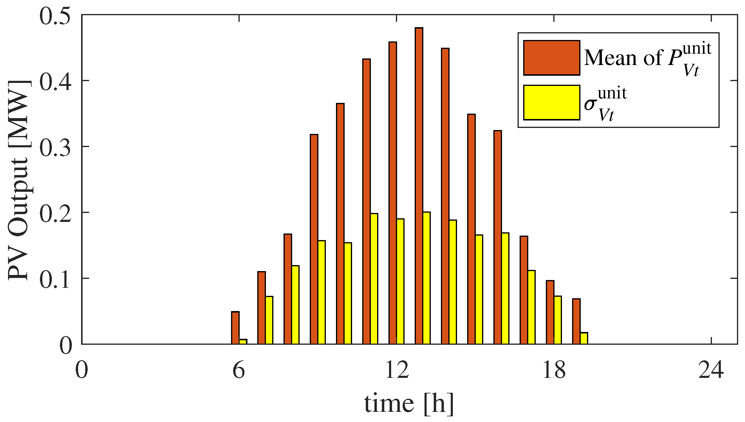
This research determines the allocation of installed PVs and ESSs for long-term. Hence, it is necessary to consider long-term changes in electricity demand and PV outputs. Moreover, it is important to consider the most severe cases of shortages and surpluses. In order to determine the allocation of facilities, we focus on grid operation for a day during which the most surplus occurred, the demand was low, and the PV output was high, because ESSs are necessary mainly to restrain power surpluses. We consider the demand on the 266th day in IEEE RTS as the minimum demand. Moreover, this research models PV outputs using actual solar irradiation data published by AMATERASS [20], and the PV output on June 2015. Figure 3 shows the mean value, , and standard deviation of PV output per unit on the date of interest.
3.3. Parameter Settings and Data
The installation target for PVs was set to 1022 MW considering 30% of the peak demand of RTS. The upper limits of both EENS and EENU, and , were set to 100 MWh/day. Note that grid operators can freely determine their requirements.
The prices of the PV and ESS, and , were 1.77 million $/MW [21] and 0.50 million $/MWh [22], respectively. This study assumed that the useful lifetimes of the PV and ESS, and , are 15 years and 10 years, respectively, and that the discount rate is 5%, even though they depend on several conditions. The penalty term for the amount of violated EENS and EENU, , should be the same as , the price of ESSs, because the relaxations of EENS and EENU play the same role as ESSs. Refer to [11] for other grid parameters, such as .
In addition, the stopping criteria of the nonlinear optimization, the number of maximum iterations, was 300. This value was employed not only in the nonlinear programing for (SP) and (SP-2), but also in the BCD method, which is the repetitive optimization between (SP-1) and (SP-2). Moreover, all the simulations in Section 4.2 are carried out on a computer with Intel(R) Core(TM) i7-6700 CPU 3.40-GHz and 32.0 GB of RAM, using MATLAB (2017a, The MathWorks, Inc., Natick, Massachusetts, MA, USA) and Matpower (Version 4.1, Power System Engineering Research Center (PSERC), USA) [23].
4. Simulation Results
This section describes the simulation results using benchmark power systems such as IEEE RTS, and thus, we verify our framework.
4.1. Results of Vulnerability Analysis
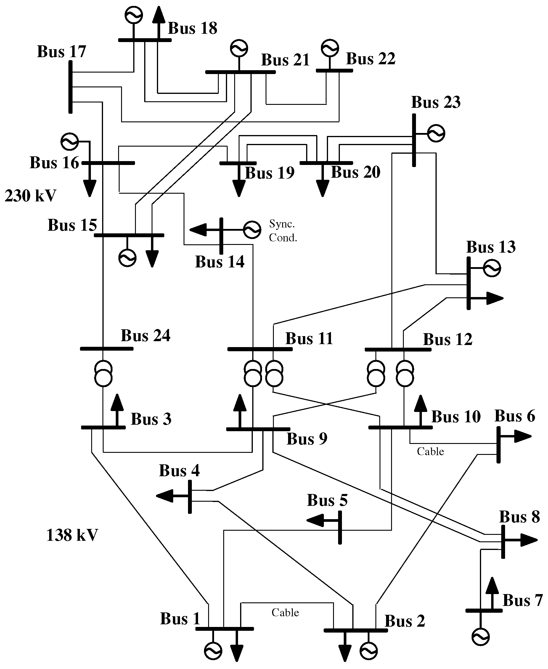
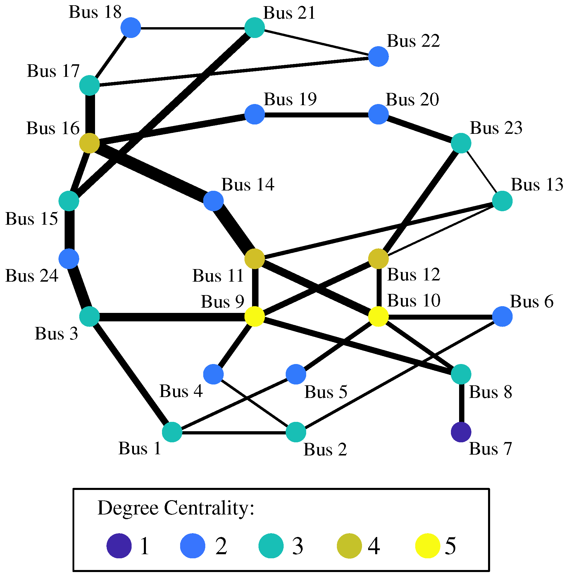
Figure 4 illustrates the IEEE RTS as an undirected graph consisting of 24 nodes and 34 edges, not 38 edges as shown in Figure 2. This is because we treat multiple edges incident onto the same two nodes as a single edge for the purpose of analysis [24]. This graph represents both degree and betweenness centrality measures using the colors of nodes and the widths of edges, respectively. The edge betweenness centrality and the probability of failure in each transmission line are also presented in Table 1, calculated using Equation (2).
Further, we determine the candidates of failures as described in Section 2.1.2. From the viewpoint of avoiding the isolation of a bus, it is evident that bus 7 is vulnerable owing to transmission line failures because the degree centrality is equal to one. Therefore, we handle the transmission line between buses 7–8. From the viewpoint of preventing cascading failures, the candidates of grid failures are as follows: transmission lines between buses 11–14, 14–16, and 15–24 because these are lines with high connected to buses with low , as presented in Figure 2 and Table 1. Notably, we exclude the edge between buses 3–24 from the candidate because it works as a transformer, and our model cannot consider the influence on voltages. In total, we consider four transmission line failures: lines between 7–8, 11–14, 14–16, and 15–24, which are set as the indices of failure, , respectively.
4.2. Results of PV and ESS Allocation
4.2.1. Case 1: Without Failures
This section describes the simulation results for the optimal allocation of PVs and ESSs without grid failures.
Figure 5 shows the allocation of PVs and ESSs, , and . The total capacity of PVs, , was 1,022 MW, thus satisfying the target. The PVs were almost evenly allocated to each bus except buses 11, 12, 17, 21, 22, and 23, because no shortages and surpluses are allowed in these buses, which do not have electricity demands. The slow ESSs were allocated to each bus evenly because the power shortages and surpluses caused by the PVs were distributed. One reason for this strategy is that the upper limit of power transmission in each line is relatively moderate, and the other is that transmission losses are not calculated in the optimization problem. Both fast ESSs for shortages and surpluses were allocated to buses with smaller PVs because the degree of uncertainty of PV outputs was smaller than that of the other buses. Moreover, the number of fast ESSs allocated for surpluses was larger than those for shortages because we focused on the most severe cases of surpluses.
4.2.2. Case 2: With Selected Failures
This section describes the allocations of PVs and ESSs considering grid failures selected in vulnerability analysis.
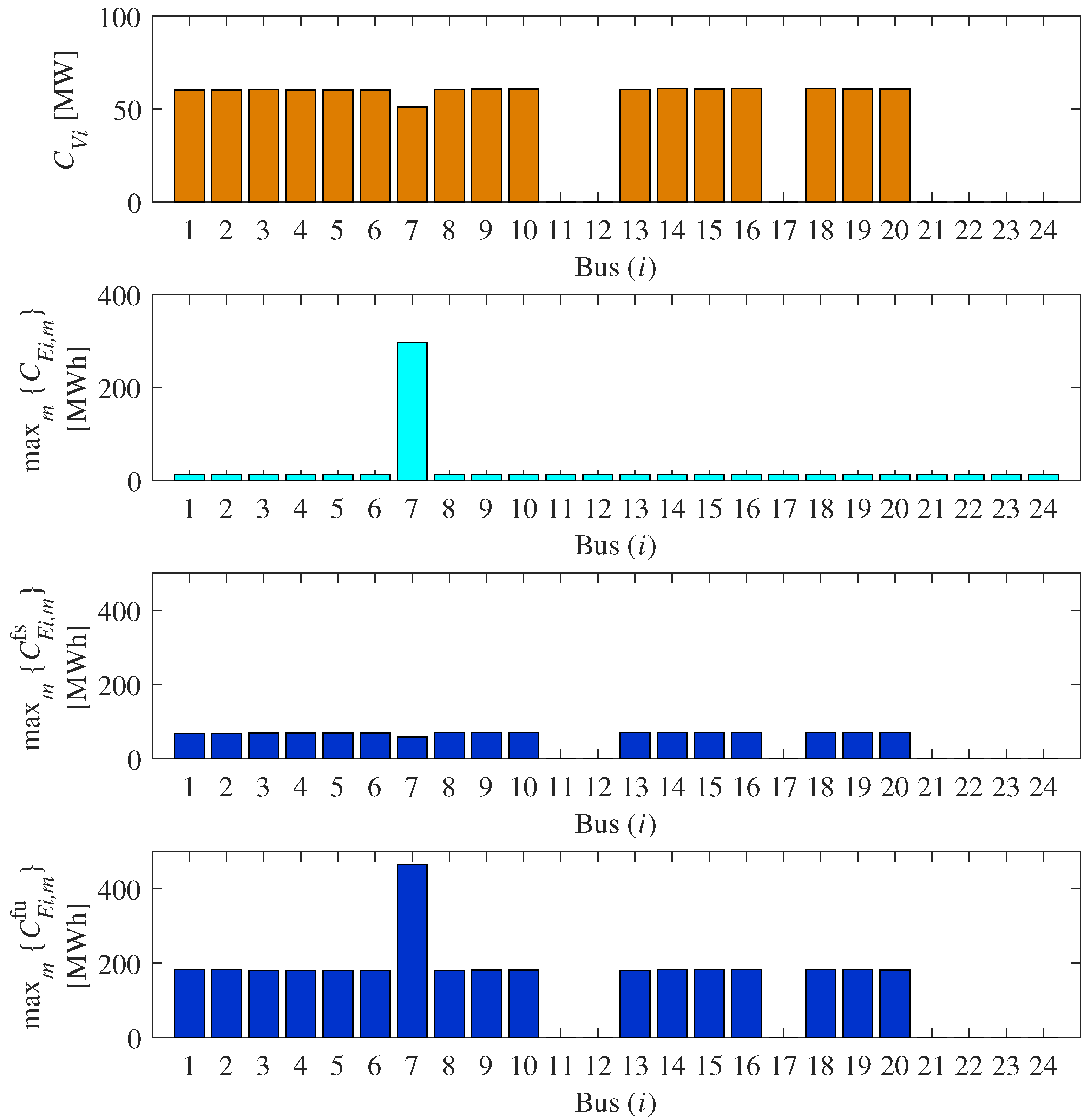
Figure 6 represents the allocation of PVs and ESSs considering failures. The sizes of slow and fast ESSs shown in Figure 6 are determined using Equation (43). The total capacity of PVs was 1022 MW, thus satisfying the target. The tendency of allocation of PVs and ESSs was similar to Case 1, except for bus 7.
Figure 7 shows the optimized allocations of slow and fast ESSs under each failure, and ().
First, the allocation of PV, slow ESS, and fast ESS for surpluses in bus 7 resulted from a failure between buses 7 and 8 (Failure ). When bus 7 is isolated, slow ESSs must be installed in bus 7 to supply electricity at night because no conventional generator is connected to bus 7, which has electricity demands. Moreover, PVs should be installed in order to reduce the number of slow ESSs installed because PVs can supply electricity in the daytime. Simultaneously, the installation of fast ESSs should be minimized when PV is installed in order to reduce the number of slow ESSs installed. Consequently, only the constraint of surpluses was relaxed because more surpluses occurred, which indicates that only fast ESSs for surpluses were allocated.
Second, the allocation of fast ESSs for shortages in bus 7 resulted from a failure between buses 15 and 24 (Failure ). Compared with the case of Failure , the results of allocation were similar for the other three failures, but the difference in failure probability had an impact on the total size of allocated ESSs, as presented in Table 2. The sizes of installed ESSs in the case of Failure were larger than those in the cases of Failures and , which have a similar tendency, because the failure probability of Failure was higher than that of others. Consequently, more fast ESSs were required to restrain shortages and surpluses owing to the more severe upper limits of EENS and EENU.
Third, however, the allocation results could not consider the impact of cascading failures caused by the failures. The major reason was that the upper limits of power transmission in these lines were relatively moderate, and consequently, an overload on transmission lines did not occur. Furthermore, the model of betweenness centrality used in this work did not consider the transmission capacity. Employing modified centrality measures will be our future work.
4.2.3. Case 3: By Comparison Method
To investigate the robustness and effectiveness, this section describes the simulation results by a comparison method with grid failures. The employed comparison method is to solve the large-scale nonlinear problem (SP) directly without dividing into two blocks.
Although to perform the simulations with four contingencies was tried, that couldn’t be solved in our environment (See Section 3.3) due to the size of problem (SP). Therefore, the allocation results considering only one fail was shown in Figure 8.
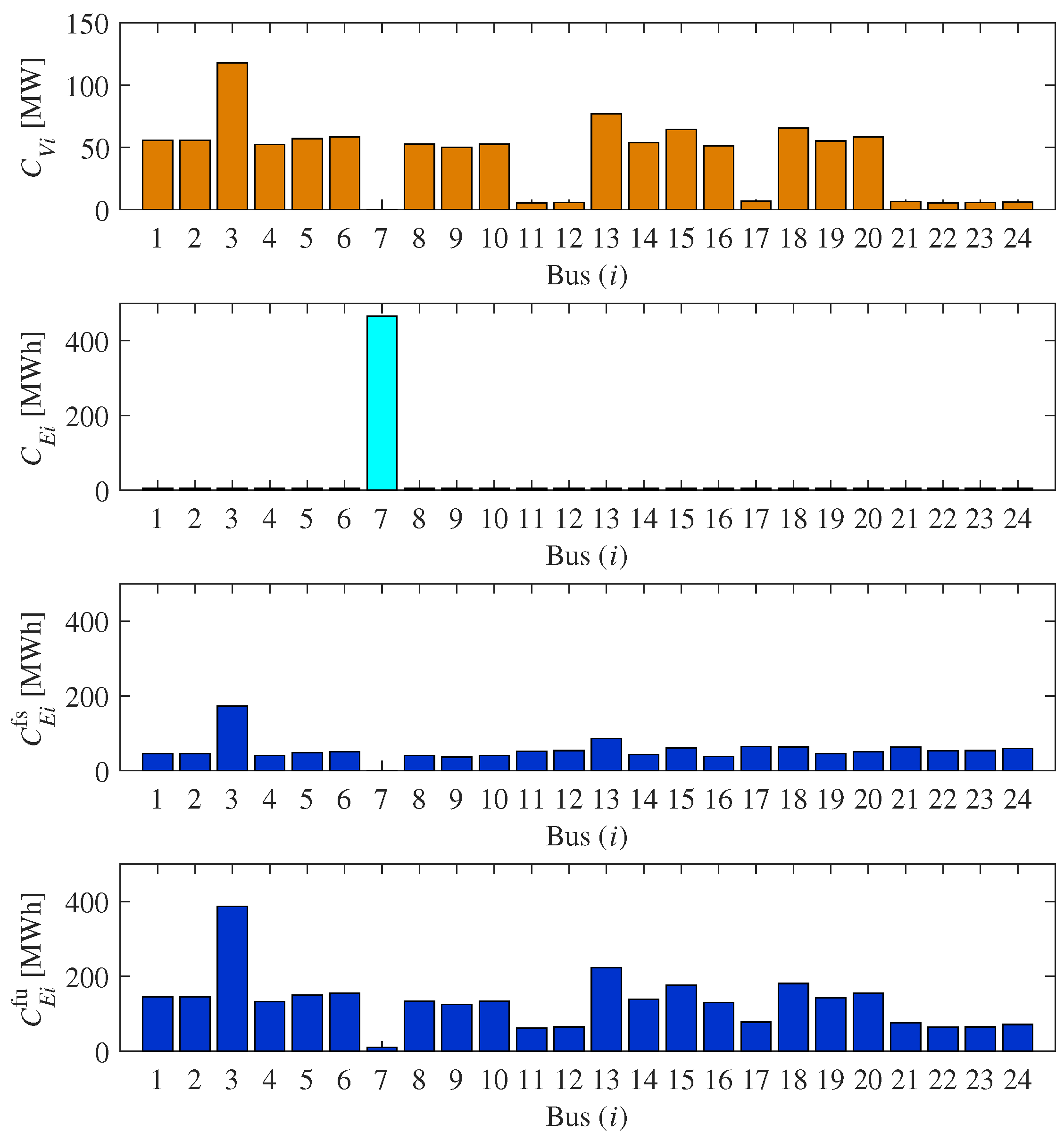
The total capacity of PVs, , was 1022 MW, thus satisfying the target. The sizes of installed slow, fast for shortage, fast for surplus ESSs were 574 MWh, 1308 MWh and 3143 MWh, respectively. The total size of ESSs was 5026 MWh.
The tendency of allocation of PVs and ESSs was similar to Case 2, but the sizes of ESSs was increased rather than the result considering failure in Case 2. Moreover, the PVs were not evenly allocated to each bus except buses 11, 12, 17, 21, 22, and 23, which resulted in the larger sizes of slow and fast ESSs. Notably, the PV was not allocated in bus 7 because this simulation considered only one failure .
The reason of the increased ESSs was because the optimization was interrupted due to the number of maximum iterations before the convergence conditions were satisfied. It is clear that this was caused by the size of the problem (SP).
As a result, it was verified that the proposed optimization scheme using the BCD method had the advantages in solution of the problem (SP).
5. Conclusions
For the development of resilient power systems under uncertainties, this research proposed a framework to determine the optimal allocations of PVs and ESSs in a power grid considering grid failures and uncertain PV outputs. The first step was to perform vulnerability analysis on the power system in order for decision makers to identify points with higher risks. We employed two centrality measures: degree centrality of nodes and betweenness centrality of edges from the viewpoint of the isolation of an area and cascading failures, respectively. The second step was to determine the allocation of PVs and ESSs considering the candidates of grid failures derived from the vulnerability analysis. We formulated the optimization problems based on the concept of “slow” and “fast” ESSs, which can play different roles in the analysis of uncertainties. Consequently, we derived the optimal allocations of PVs and ESSs under the uncertainties including the selected grid failures and PV outputs, and especially, slow ESS reflected the influences of grid failures.
Our future work will employ other centrality measures that can consider the configuration of power systems such as the capacity of a transmission line. Furthermore, other types of probability distributions will be considered when evaluating the probabilistic indices. Moreover, the formulation in this study utilized DC-OPF, which cannot consider a variation of voltages and transmission losses; however, our future work will extend the formulation to one with AC-OPF, which can introduce the above conditions. This future work will facilitate the solution of similar optimization problems in not only transmission systems, but also distribution systems.
Acknowledgments
This work was supported in part by the Program for Leading Graduate Schools, “Science for Development of Super Mature Society” and Japan Science and Technology Agency (JST), CREST Grant Number JPMJCR15K5.
Author Contributions
All the authors contributed equally to the design and writing process of this publication.
Conflicts of Interest
The authors declare no conflict of interest.
Abbreviations
Indices and Sets:
| i | Index of buses, running from 1 to |
| l | Index of transmission lines, running from 1 to |
| k | Index of conventional generators, running from 1 to |
| m | Index of grid failures, running from 1 to |
| t | Index of time, running from 1 to |
| Set of buses in power systems | |
| Set of conventional generators () | |
| Set of buses with demands () |
Decision variables:
| Output of the k th conventional generator at t | |
| Total output of conventional generators in bus i at t | |
| Capacity of PVs in bus i | |
| Capacity of slow ESSs in bus i at t | |
| Capacity of fast ESSs for shortages and surpluses in bus i at t, respectively | |
| Mismatch of power demand and supply in bus i at t | |
| Scheduling of slow ESSs in bus i at t | |
| Scheduling of fast ESSs for shortages and surpluses in bus i at t, respectively | |
| Inflow/outflow power in bus i at t | |
| Phase angle in bus i at t | |
| State of charge of slow ESSs in bus i at t | |
| Relaxation of power shortages and surpluses for 1 h in bus i at t, respectively | |
| Vector of decision variables related to allocation of PV and ESS | |
| Vector of decision variables related to grid operation |
Parameters:
| Degree centrality of bus i | |
| Adjacency matrix of a power system and its element, respectively | |
| Betweenness centrality for the l th transmission line | |
| Number of shortest paths between buses i and j including the l th transmission line | |
| Total number of shortest paths between buses i and j | |
| Polynomial coefficient of the n th term in a fuel cost function of the k th generator | |
| r | Discount rate |
| Useful lifetime of ESSs and PVs in years, respectively | |
| Price of ESSs and PVs, respectively | |
| Installation target of PVs | |
| Output of PV per unit in bus i at t | |
| Electricity demand in bus i at t | |
| Susceptance between buses i and j | |
| Capacity of transmission line between buses i and j | |
| Upper limits of power shortages and surpluses for 1 h in bus i at t | |
| Generator connection matrix and its element, respectively | |
| Minimum and maximum output of the k th generator, respectively | |
| Maximum difference of the k th generator for 1 h | |
| Standard deviation of PV output in bus i at t for 1 h | |
| Penalty term for the violation of constraints of EENS and EENU |
Functions and others:
| Probability density function of Gaussian distribution | |
| Error function | |
| Function of EENS and EENU for 1 h in bus i at t, respectively | |
| Probability of the m th grid failure | |
| Estimated value of stochastic variable x | |
| Mean value of stochastic variable x | |
| Optimal value in the previous step in BCD Method |
References
- Zheng, L.; Hu, W.; Lu, Q.; Min, Y. Optimal energy storage system allocation and operation for improving wind power penetration. IET Gener. Transm. Distrib. 2015, 9, 2672–2678. [Google Scholar] [CrossRef]
- Ghofrani, M.; Arabali, A.; Etezadi-Amoli, M.; Fadali, M.S. Energy storage application for performance enhancement of wind integration. IEEE Trans. Power Syst. 2013, 28, 4803–4811. [Google Scholar] [CrossRef]
- Wogrin, S.; Gayme, D.F. Optimizing storage siting, sizing, and technology portfolios in transmission-constrained networks. IEEE Trans. Power Syst. 2015, 30, 3304–3313. [Google Scholar] [CrossRef]
- Vovos, P.N.; Harrison, G.P.; Wallace, A.R.; Bialek, J.W. Optimal power flow as a tool for fault level-constrained network capacity analysis. IEEE Trans. Power Syst. 2005, 20, 734–741. [Google Scholar] [CrossRef]
- Masaud, T.M.; Mistry, R.D.; Sen, P.K. Placement of large-scale utility-owned wind distributed generation based on probabilistic forecasting of line congestion. IET Renew. Power Gener. 2017, 11, 979–986. [Google Scholar] [CrossRef]
- Zhang, B.; Dehghanian, P.; Kezunovic, M. Optimal allocation of pv generation and battery storage for enhanced resilience. IEEE Trans. Smart Grid. [CrossRef]
- Konishi, R.; Takahashi, M. Optimal allocation of photovoltaic systems and energy storages in power systems considering power shortage and surplus. In Proceedings of the 9th International: 2014 Electric Power Quality and Supply Reliability Conference (PQ), Rakvere, Estonia, 11–13 June 2014; pp. 127–132. [Google Scholar]
- Billinton, R.; Allan, R. Reliability Evaluation of Power Systems, 1 ed.; Springer: New York, NY, USA, 1996. [Google Scholar]
- Dent, C.J.; Ochoa, L.F.; Harrison, G.P.; Bialek, J.W. Efficient secure AC OPF for network generation capacity assessment. IEEE Trans. Power Syst. 2010, 25, 575–583. [Google Scholar] [CrossRef] [Green Version]
- Konishi, R.; Takahashi, M. Optimal facility allocation and determination of demand response participation rate considering uncertainties in power systems. Trans. Inst. Syst. Control Inf. Eng. 2017, 30, 10–19. [Google Scholar] [CrossRef]
- Subcommittee, P.M. IEEE reliability test system. IEEE Trans. Power Appar. Syst. 1979, PAS-98, 2047–2054. [Google Scholar] [CrossRef]
- Baldick, R.; Chowdhury, B.; Dobson, I.; Dong, Z.; Gou, B.; Hawkins, D.; Huang, Z.; Joung, M.; Kim, J.; Kirschen, D.; et al. Vulnerability assessment for cascading failures in electric power systems. In Proceedings of the 2009 IEEE/PES Power Systems Conference and Exposition, Seattle, WA, USA, 15–18 March 2009; pp. 1–9. [Google Scholar]
- Bompard, E.; Pons, E.; Wu, D. Extended topological metrics for the analysis of power grid vulnerability. IEEE Syst. J. 2012, 6, 481–487. [Google Scholar] [CrossRef]
- Girvan, M.; Newman, M.E.J. Community structure in social and biological networks. Proc. Natl. Acad. Sci. USA 2002, 99, 7821–7826. [Google Scholar] [CrossRef] [PubMed]
- Freeman, L.C. A set of measures of centrality based on betweenness. Sociometry 1977, 40, 35. [Google Scholar] [CrossRef]
- Snyder, L. Multi-period optimal power flow problems. Optima 2013, 93, 8–9. [Google Scholar]
- Stott, B.; Jardim, J.; Alsac, O. DC power flow revisited. IEEE Trans. Power Syst. 2009, 24, 1290–1300. [Google Scholar] [CrossRef]
- Wang, P.; Gao, Z.; Tjernberg, L.B. Operational adequacy studies of power systems with wind farms and energy storages. In Proceedings of the 2013 IEEE Power Energy Society General Meeting, Vancouver, BC, Canada, 21–25 July 2013. [Google Scholar]
- Grippo, L.; Sciandrone, M. On the convergence of the block nonlinear Gauss-Seidel method under convex constraints. Oper. Res. Lett. 2000, 26, 127–136. [Google Scholar] [CrossRef]
- AMATERASS. Specified Nonprofit Corporation Solar Radiation Consortium. Available online: http://www.amaterass.org/ (accessed on 1 August 2017). (In Japanese).
- Chung, D.; Davidson, C.; Fu, R.; Ardani, K.; Margolis, R. U.S. Photovoltaic Prices and Cost Breakdowns: Q1 2015 Benchmarks for Residential, Commercial, and Utility-Scale Systems; Technical Report September; National Renewable Energy Laboratory: Golden, CO, USA, 2015.
- Deloitte. Energy Storage: Tracking the Technologies That Will Transform the Power Sector. Available online: https://www2.deloitte.com/content/dam/Deloitte/us/Documents/energy-resources/us-er-energy-storage-tracking-technologies-transform-power-sector.pdf (accessed on 15 August 2017).
- Zimmerman, R.; Murillo Sánchez, C.; Thomas, R. MATPOWER: Steady-state operations, planning, and analysis tools for power systems research and education. IEEE Trans. Power Syst. 2011, 26, 12–19. [Google Scholar] [CrossRef]
- Zio, E.; Golea, L.R. Analyzing the topological, electrical and reliability characteristics of a power transmission system for identifying its critical elements. Reliab. Eng. Syst. Saf. 2012, 101, 67–74. [Google Scholar] [CrossRef] [Green Version]
Figure 1.
Proposed Framework to Determine Optimal Allocations of PVs and ESSs.
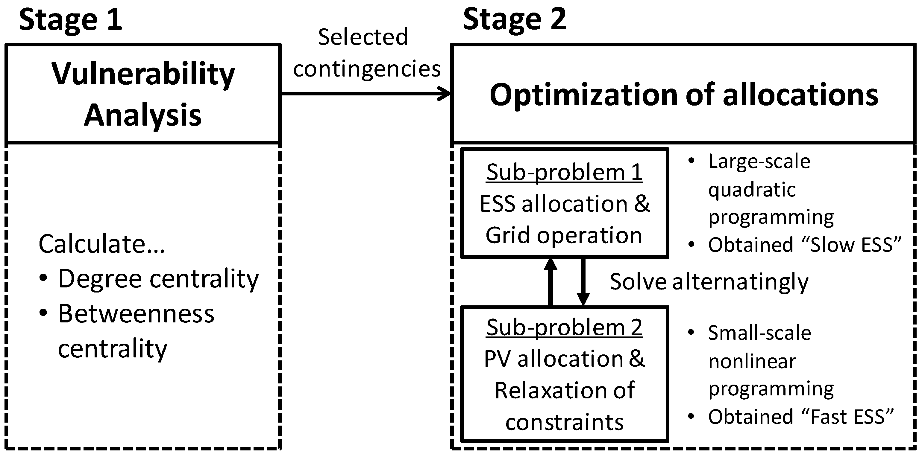
Figure 2.
IEEE Reliability Test System [11].
Figure 2.
IEEE Reliability Test System [11].

Figure 3.
Mean and Standard Deviation of PV Outputs.

Figure 4.
Topological graph of IEEE RTS.

Figure 5.
Allocation of PVs and ESSs without grid failures.
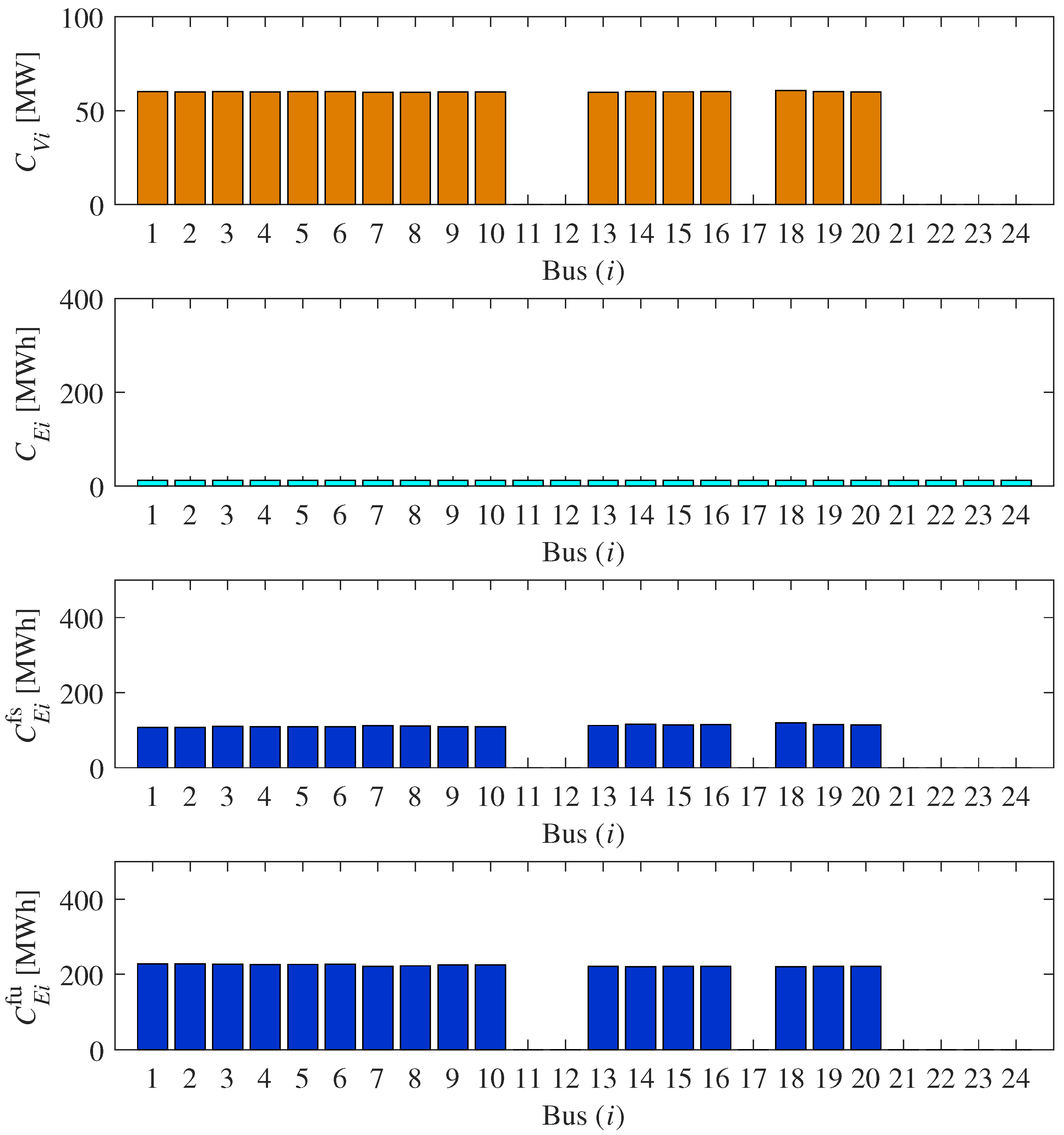
Figure 6.
Allocation of PVs and ESSs considering grid failures.

Figure 7.
Allocation of Slow ESSs considering grid failures.
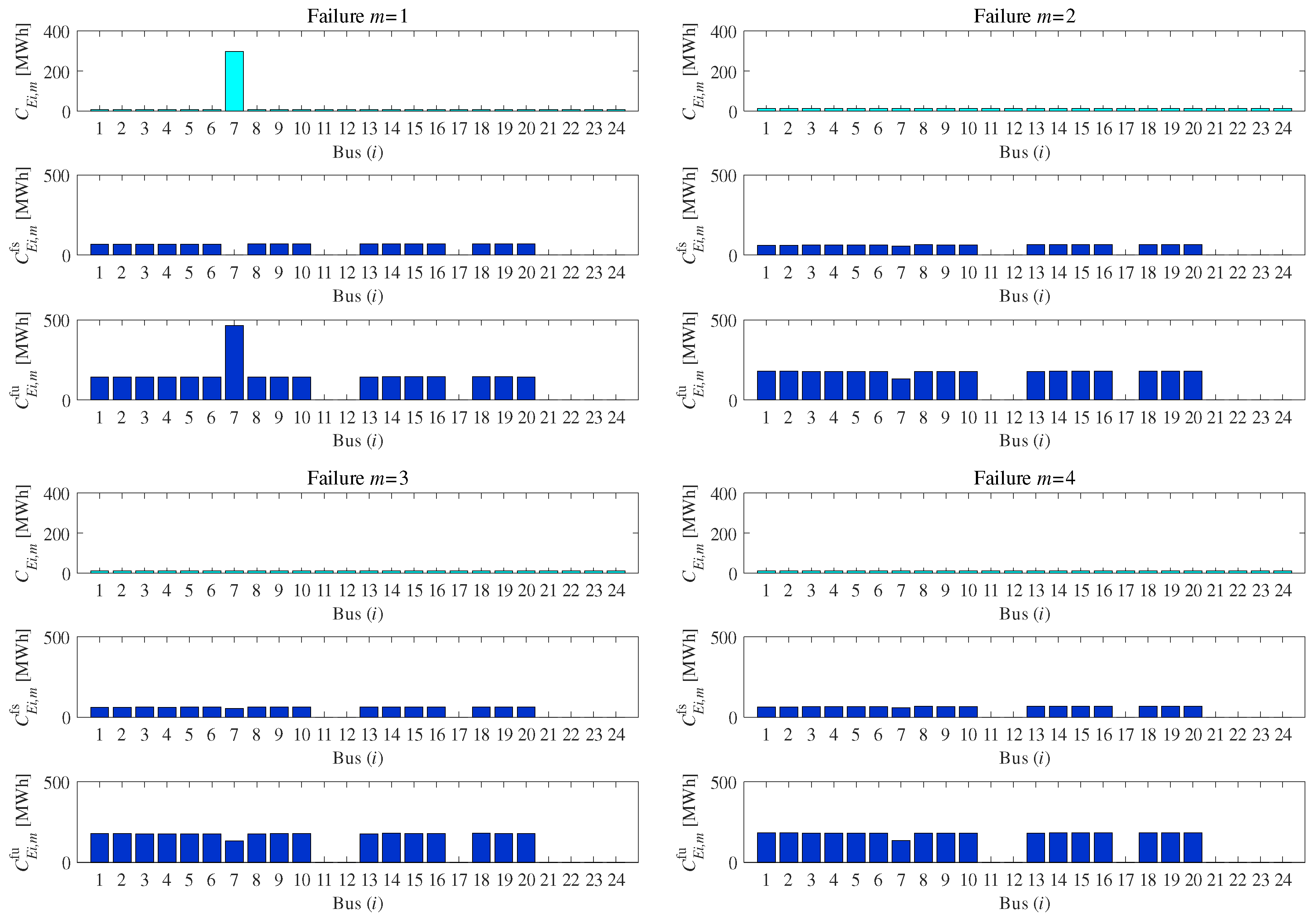
Figure 8.
Allocation of PVs and ESSs considering failure by comparison method.


Table 1.
Transmission Lines in RTS and Betweenness Centrality.
| l | From Bus | To Bus | l | From Bus | To Bus | ||||
|---|---|---|---|---|---|---|---|---|---|
| 1 | 1 | 2 | 7.4 | 0.24 | 18 | 11 | 13 | 9.0 | 0.40 |
| 2 | 1 | 3 | 14.8 | 0.51 | 19 | 11 | 14 | 30.8 | 0.39 |
| 3 | 1 | 5 | 6.9 | 0.33 | 20 | 12 | 13 | 4.0 | 0.40 |
| 4 | 2 | 4 | 5.3 | 0.39 | 21 | 12 | 23 | 14.4 | 0.52 |
| 5 | 2 | 6 | 6.3 | 0.48 | 22 | 13 | 23 | 3.0 | 0.49 |
| 6 | 3 | 9 | 19.2 | 0.38 | 23 | 14 | 16 | 28.3 | 0.38 |
| 7 | 3 | 24 | 25.3 | 0.02 | 24 | 15 | 16 | 14.9 | 0.33 |
| 8 | 4 | 9 | 12.5 | 0.36 | 25 | 15 | 21 | 17.4 | 0.41 |
| 9 | 5 | 10 | 10.1 | 0.34 | 26 | 15 | 24 | 22.8 | 0.41 |
| 10 | 6 | 10 | 11.5 | 0.33 | 27 | 16 | 17 | 22.6 | 0.35 |
| 11 | 7 | 8 | 11.5 | 0.30 | 28 | 16 | 19 | 15.0 | 0.34 |
| 12 | 8 | 9 | 13.6 | 0.44 | 29 | 17 | 18 | 7.3 | 0.32 |
| 13 | 8 | 10 | 10.0 | 0.44 | 30 | 17 | 22 | 7.3 | 0.54 |
| 14 | 9 | 11 | 14.4 | 0.02 | 31 | 18 | 21 | 4.7 | 0.35 |
| 15 | 9 | 12 | 13.6 | 0.02 | 32 | 19 | 20 | 11.4 | 0.38 |
| 16 | 10 | 11 | 17.9 | 0.02 | 33 | 20 | 23 | 13.9 | 0.34 |
| 17 | 10 | 12 | 11.4 | 0.02 | 34 | 21 | 22 | 4.7 | 0.45 |
Table 2.
Capacities of ESSs considering failures.
| Type of ESS | Allocated | Derived under the mth Failure | |||
|---|---|---|---|---|---|
| Capacity | |||||
| Slow | 587 | 469 | 302 | 302 | 302 |
| Fast for Shortage | 1168 | 1110 | 1082 | 1058 | 1128 |
| Fast for Surplus | 3370 | 2994 | 2970 | 2970 | 3040 |
| Total | 5126 | 4573 | 4354 | 4330 | 4470 |
© 2017 by the authors. Licensee MDPI, Basel, Switzerland. This article is an open access article distributed under the terms and conditions of the Creative Commons Attribution (CC BY) license (http://creativecommons.org/licenses/by/4.0/).
Share and Cite
MDPI and ACS Style
Konishi, R.; Takahashi, M. Optimal Allocation of Photovoltaic Systems and Energy Storage Systems based on Vulnerability Analysis. Energies 2017, 10, 1477. https://doi.org/10.3390/en10101477
AMA Style
Konishi R, Takahashi M. Optimal Allocation of Photovoltaic Systems and Energy Storage Systems based on Vulnerability Analysis. Energies. 2017; 10(10):1477. https://doi.org/10.3390/en10101477
Chicago/Turabian StyleKonishi, Ryusuke, and Masaki Takahashi. 2017. "Optimal Allocation of Photovoltaic Systems and Energy Storage Systems based on Vulnerability Analysis" Energies 10, no. 10: 1477. https://doi.org/10.3390/en10101477
Note that from the first issue of 2016, this journal uses article numbers instead of page numbers. See further details here.