Economic Microgrid Planning Algorithm with Electric Vehicle Charging Demands

Abstract

Two of the most important technologies for future power systems to reduce greenhouse gas are electric vehicles (EVs) and renewable generation. When EVs become more common, the overall demand of electricity will significantly increase because EVs consume a large amount of electricity. Also, a daily load curve with EVs heavily depends on how much electricity EVs consume and when electricity is consumed. The microgrid is an important technology to promote renewable generation, and the increased demand and changed load curve should be considered in the microgrid planning stage to install robust and economical microgrids. In this paper, we propose an algorithm for microgrid planning with EV charging demand to find the most economical configuration through which to maximally utilize renewable generation. The algorithm uses a renewable generation-following EV charging scheme and HOMER. Through simulations, it is shown that the microgrid constructed by the proposed algorithm reduces the investment cost and CO₂ emission.

1. Introduction

Sustainable development is one of the key engineering challenges for future society. To this end, 195 countries agreed in December 2015 to reduce greenhouse gas through the Paris agreement [1]. According to the agreement, Korea must reduce greenhouse emissions 37% by 2030 compared to that of business-as-usual (BAU). From the perspective of the power system, two of the most vital technologies to reduce greenhouse gas are electric vehicles (EVs) and renewable generation. Note that in this paper, an EV indicates any battery-type plug-in electric vehicle such as a plug-in hybrid electric vehicle (PHEV) or plug-in electric vehicle (PEV).

EVs are receiving attention as a promising alternative to the fossil fuel-based vehicles that are one of the major causes of the greenhouse effect [2]. However, since EVs consume a very high amount of electricity during the charging period, the power system will be exposed to considerable stress when EVs become widespread [3]. It has been shown that simple electricity price rates such as time-of-use (TOU) pricing induce a new rebound peak in the off-peak hours because most EVs are mainly charged during that period [4].

Many studies have been conducted on reducing the stress on the grid by distributing the EV charging demand, i.e., the EV charging scheduling issue [4,5,6,7,8,9,10,11]. Distributing methods for EV charging demands can be classified into centralized [5,6,7,8] or decentralized [9,10,11] schemes. In [5], a real-time EV charging scheme has been proposed to improve voltage profile through centralized charging control. In addition, the authors of [6] have proposed various objective functions such as total feeder losses, total cost of energy, and total cost of PEV charging to protect the distribution grid. To reduce computational complexity, a scalable EV charging scheduling scheme has been proposed through Model Predictive Control (MPC) by using statistical information [7]. In [8], a semi-centralized scheme has been proposed in which, on behalf of each EV owner, a fleet operator interacts with a distribution system operator to determine the hourly electricity price. Conversely, in [9,10,11], a decentralized scheme has been proposed. The EV scheduling was modeled as a Stackelberg game, in which the players are an electricity retailer and EV customers [9]. In [10], an optimal EV charging scheme has been proposed to fill the valleys of electric load curve. Last, with an assumption of predictable EV user’s behavior, an optimal EV scheduling has been proposed with discrete EV charging levels [11].

The microgrid is a vital technology to promote renewable generation to the power system. It is defined as a group of interconnected loads and distributed energy resources with clearly defined electrical boundaries. The two major advantages of the microgrid are: (i) a number of distributed generations can be adopted in the grid through the microgrid [12]; and (ii) the microgrid improves the grid resilience against disasters [13].

Since microgrids include fewer households and consume less electricity than a main grid, the adoption of EVs in a microgrid will have a more serious impact. Therefore, EV charging in microgrids should be precisely controlled to ensure their economy and resilience. To this end, recent studies have investigated the EV charging issue in the microgrid [14,15].

The optimal microgrid planning problem has been investigated through simulation tools such as HOMER and WebOpt [16,17], or through numerical analysis by considering uncertainties in the future [18,19,20]. In [18], an optimal microgrid planning problem has been proposed for island-mode microgrids while a similar optimization problem has been proposed for grid-connected microgrids in [19]. Another optimization problem for microgrid planning has been proposed that minimizes risk rather than cost [20].

EV charging demands will significantly change the load curve in microgrid, so we should consider EV charging scheduling schemes in the microgrid planning stage. To the best of our knowledge, however, none of the studies consider the load curve changes due to the EVs in the microgrid planning stage.

In this paper, the microgrid planning problem with EV charging demands is investigated. Three main contributions of this work are: (i) we derive load curves from several EV charging scheduling schemes; (ii) optimal microgrid configurations for above charging schemes are investigated using HOMER; and (iii) we propose an algorithm for microgrid planning that maximally uses renewable generators. The proposed algorithm iteratively searches between an optimal EV charging schedule and an optimal microgrid configuration. Through simulations, it is shown that the microgrid constructed by the proposed algorithm reduces the investment cost and CO₂ emission by controlling the EV charging demands effectively.

The remainder of the paper is organized as follows. We first describe EV charging scheduling schemes in Section 2. Then, the optimal microgrid planning problem by using HOMER is shown in Section 3. Using the renewable generation-following EV charging scheme and HOMER, we propose an algorithm for microgrid planning in Section 4. After evaluating case studies in Section 5, we conclude our paper in Section 6.

2. EV Charging Scheduling Schemes

In this section, the EV charging model is described and the four EV charging scheduling schemes are then shown.

2.1. EV Charging Model

We consider a set $\mathcal{N}$ of EVs in a microgrid. Each day is divided into $H$ time periods. A period set and period index are denoted as $\mathscr{H}=\{1,2,\cdots ,H\}$ and $h$, respectively. Let $x_i^h$ denote the amount of electricity consumption by customer $i$ at time $h$ to charge the EV in units of kW. It is assumed that all EVs are charged at home and on campus for the residential microgrid and campus microgrid, respectively.

The charging requirement of each EV $i$ is a full charging of its battery before departure. This can be modeled as

$$\begin{array}{ll}\multicolumn{2}{c}{{\displaystyle \sum _{h\in {\mathcal{T}}_i}{\mu }_c}{x}_i^h=E_i,}\\ 0\le x_i^h\le {\delta }_i,& \mathrm{if}h\in {\mathcal{T}}_i,\\ x_i^h=0,& \mathrm{if}h\notin {\mathcal{T}}_i.\end{array}$$

(1)

where ${\mu }_c$, $E_i$, and ${\delta }_i$ denote the battery charging efficiency, electricity in kWh required for full charging of EV $i$, and the maximum charging rate of EV $i$, respectively. The charging period for EV $i$ starts at ${\alpha }_i$ and ends at ${\beta }_i$. Let ${\mathcal{T}}_i=[{\alpha }_i,{\beta }_i]$ denote the set of time periods in which EV $i$ is at the place of charging, i.e., at home or on campus.

2.2. Min Time Charging Scheduling Scheme

The most naïve charging scheduling scheme is that EVs are charged as soon as possible. That is, when an EV is parked at home or on campus, it is charged with ${\delta }_i$ charging rate until fully charged. In this paper, we call this scheme the “min time charging scheduling scheme” [21]. It is important to note that this scheme does not require interaction between customers and control entities such as the microgrid energy management system (EMS) and fleet operator, i.e., it is an uncontrolled charging scheme.

2.3. Min Cost Charging Scheduling Scheme

Currently, utility companies provide special electricity price rates for EV charging demand. In general, they provide TOU rates by dividing one day into peak, partial-peak, and off-peak periods.

Table 1. Electric Vehicle (EV) Charging Price Rate for Pacific Gas and Electric Company (PG&E) and Korea Electric Power Corporation (KEPCO).

Utility Company	Off-Peak Period	Partial-Peak Period	Peak Period
PG&E	[11 p.m., 7 a.m.]	[7 a.m., 2 p.m.], [9 p.m., 10 p.m.]	[2 p.m., 9 p.m.]
	0.099 $/kWh	0.226 $/kWh	0.428 $/kWh
KEPCO	[11 p.m., 9 a.m.]	[9 a.m., 10 a.m.], [12 p.m., 1 p.m.], [5 p.m., 11 p.m.]	[10 a.m., 12 p.m.], [1 p.m., 5 p.m.]
	0.048 $/kWh 1	0.121 $/kWh	0.194 $/kWh

¹ We use the exchange rate of $1 = 1200 Won.

shows two EV charging price rate examples for Pacific Gas and Electric Company (PG&E) in the US [22] and Korea Electric Power Corporation (KEPCO) in Korea [23] during the summer season. There is another type of electricity pricing rate named real-time pricing (RTP), which announces hourly price rate for the next day. Southern California Edison (SCE) in the US currently offers RTP in which the hourly price is decided from past daily load data and weather data. Note that a graph of RTP and SMP in one day of summer 2014 in Korea in Section 5 shows examples of TOU and RTP price rates offered by KEPCO.

The second uncontrolled EV charging scheme is the cost minimization charging scheduling scheme, called the “min cost charging scheduling scheme”. In this charging scheme, customers decide the amount of electricity for the EV charging in each period to minimize the cost of electricity [24]. Since we consider two price rates, i.e., TOU rate and RTP, they are called “min cost1” and “min cost2”, respectively. The optimization problem can be formulated as

$$({\mathrm{U}}_i)\underset{x_i^h}{\min }\sum _{h\in {\mathcal{T}}_i}{p}^h·x_i^h$$

(2)

$$\begin{array}{lll}\mathrm{subject}\mathrm{to}\hfill & \multicolumn{2}{c}{{\displaystyle \sum _{h\in {\mathcal{T}}_i}{\mu }_c}{x}_i^h=E_i,}\\ \hfill & 0\le x_i^h\le {\delta }_i,\hfill & \mathrm{if}h\in {\mathcal{T}}_i,\\ \hfill & x_i^h=0,\hfill & \mathrm{if}h\notin {\mathcal{T}}_i.\end{array}$$

where $p^h$ is the electricity price rate at time $h$. It is assumed that the electricity price rate of the day is known to all customers.

The control variable for the problem $({\mathrm{U}}_i)$ is only related to each customer $i$ and it does not depend on other customers’ charging behaviors. Therefore, each customer decides his/her charging scheduling. That is, this scheme does not require real-time interaction between each customer and the control entity. The only information for customer $i$ needed to solve the problem $({\mathrm{U}}_i)$ is the electricity price rate of the day.

Generally, the problem $({\mathrm{U}}_i)$ can have many solutions. and we choose the one which has the fastest charging end time because it is the most convenient solution for the EV owner.

2.4. Min Var Charging Scheduling Scheme

In the microgrid case, another important metric is the peak electricity demand, since the microgrid should be planned to fulfill the peak demand. Therefore, we choose the objective to be minimizing the maximum demand of one-day load. In general, the problem has more than one solution, so we choose the one that minimizes the variance of one-day load. We call this the “min Var charging scheduling scheme”.

To this end, the amount of base load, denoted by $x_0^h$, as well as EV loads should be considered together. We formulate the optimization problem as

$$(\mathrm{C})\underset{x_i^h,i\in \mathcal{N}}{\min }\mathrm{Var}(X^h)$$

(3)

$$\begin{array}{lll}\mathrm{subject}\mathrm{to}\hfill & {\displaystyle \sum _{h\in {\mathcal{T}}_i}{\mu }_c}{x}_i^h=E_i,\hfill & \forall i\in \mathcal{N},\hfill \\ \hfill & 0\le x_i^h\le {\delta }_i,\hfill & \mathrm{if}h\in {\mathcal{T}}_i,\forall i\in \mathcal{N},\\ \hfill & x_i^h=0,\hfill & \mathrm{if}h\notin {\mathcal{T}}_i,\forall i\in \mathcal{N}.\end{array}$$

where $X^h$ and $\mathrm{Var}(X^h)$ are the total electricity consumption at $h$ and its variance, respectively. They are defined as $X^h=x_0^h+{\displaystyle \sum _{i\in \mathcal{N}}{x}_i^h}$ and $\mathrm{Var}(X^h)=\frac{1}{H}{\displaystyle \sum _h{(X^h-\mu )}^2}$.

The problem $(\mathrm{C})$ is a standard convex optimization problem, so we can get its solution. Detailed procedures and the closed form solution for the problem $(\mathrm{C})$ are presented in Appendix A.

The control variable for this optimization problem is the charging rates for all of the EVs in the microgrid. Therefore, the problem $(\mathrm{C})$ requires a central control entity in order to obtain the optimal solution and to distribute power to all customers.

Note that, in [15], the EV scheduling problem of minimizing the load variance was proposed without showing its closed form solution, while this work derived the closed form solution for $(\mathrm{C})$. Also, the target of [15] is the EV scheduling in the case of one house while the target of this work is microgrid planning.

2.5. Max Renewable Charging Scheme

Since a number of renewable generations will be adopted in a microgrid [12], one key goal for charging scheduling in a microgrid is a maximum use of the renewable generations. Mathematically, the objective of this scheduling scheme is to minimize the difference between electric load and the renewable generation output by controlling the EV charging demands. We call this “max renewable charging scheduling scheme”.

Since the power output of renewable generation displays randomness, we use an expected value for the output of a renewable generation. Let $R^h$ denote a random variable defined to be the output of renewable generations at time $h$, and recall that the total electricity consumption at $h$ is $X^h$, which consists of base load and EV charging load. Then, we formulate the optimization problem as

$$(\mathrm{R})\underset{x_i^h,i\in \mathcal{N}}{\min }{(X^h-E(R^h\left)\right)}^2$$

$$\begin{array}{lll}\mathrm{subject}\mathrm{to}\hfill & {\displaystyle \sum _{h\in {\mathcal{T}}_i}{\mu }_c}{x}_i^h=E_i,\hfill & \forall i\in \mathcal{N},\hfill \\ \hfill & 0\le x_i^h\le {\delta }_i,\hfill & \mathrm{if}h\in {\mathcal{T}}_i,\forall i\in \mathcal{N},\hfill \\ \hfill & x_i^h=0,\hfill & \mathrm{if}h\notin {\mathcal{T}}_i,\forall i\in \mathcal{N}.\hfill \end{array}$$

We assume that the type and capacity of renewable generations in the microgrid are given. Like the problem $(\mathrm{C})$, the problem $(\mathrm{R})$ is a standard convex optimization problem, so we can get the solution. Because of the space limit, we omit the detailed procedure.

3. Microgrid Planning Problem

When the EV charging demand is added to the base load, the load curve significantly changes. The optimal microgrid planning problem for the changed load is described in this section. We use HOMER Energy software to obtain the optimal microgrid configurations.

3.1. HOMER Energy

HOMER energy software was originally developed by the US National Renewable Energy Laboratory (NREL) and is commercially available [25]. It is a simulation tool used to find the optimal combination of generations for a microgrid. For this software, basic parameters need to be manually set, including electrical load, diesel price, solar and wind resources, generation capacities, system costs for each generation, etc. The term ‘optimal’ in HOMER means that the obtained solution has the lowest total net present cost (NPC) [26] to build the microgrid. The total NPC is mathematically defined as

$$\mathrm{Total}\mathrm{NPC}={\displaystyle \sum _{t=0}^M\frac{C_{ann}}{{(1+r)}^t}}.$$

(4)

where $M$, $r$, and $C_{ann}$ are the project lifetime, discount rate, and the total annualized cost during the project lifetime, respectively.

Note that, to obtain the optimal microgrid configuration, HOMER uses an exhaustive search algorithm that simply calculates the NPCs of all candidate solutions and chooses the one with the lowest NPC as an optimal solution [27].

3.2. Microgrid Component Modeling

We consider the possible energy supply options to be solar photovoltaics (PV), wind turbine, diesel generator, battery, and alternating current (AC)/direct current (DC) converter.

Table 2. Unit Component Cost for Microgrid Configuration.

Generators	Capital Cost ($)	Replacement Cost ($)	O&M Cost ($/yr)
Solar PV (20 kW)	60,000	60,000	200
Wind turbine (20 kW)	100,000	100,000	1000
Diesel (50 kW)	25,000	25,000	13,000
Battery (20 kWh)	6000	6000	200
Converter (20 kW)	6000	6000	0

shows the system cost for each generator obtained in [28] and default value. The system cost comprises capital cost, replacement cost, and operation and maintenance (O&M) cost.

The load profiles for the targeted areas include the base load and EV charging demand. The base load curves are obtained from [29], which is an electricity consumption measurement report by the Korean government. The load curves for EV charging are obtained as shown in Section 2 for the various charging schemes. Also, the daily noise of 15% and hourly noise of 20% are added to the load.

The daily solar radiation data for Seoul, Korea (37°34′ N, 126°58′ E) are obtained from the National Aeronautics and Space Administration (NASA) Surface Meteorology and Solar Energy website [30]. The annual average daily solar radiation for Seoul is 4.05 kWh/m²/day. The maximum and minimum values are 5.54 kWh/m²/day and 2.44 kWh/m²/day in May and December, respectively. The diesel price is set as $1.22 per liter, which is obtained from the diesel price monitoring website [31]. The project life time of 25 years and the annual interest rate of 6.0% are used.

4. Max Renewable Microgrid Planning Algorithm

To construct a robust and economical microgrid with EVs, we propose an algorithm for microgrid planning that uses renewable generation as much as possible.

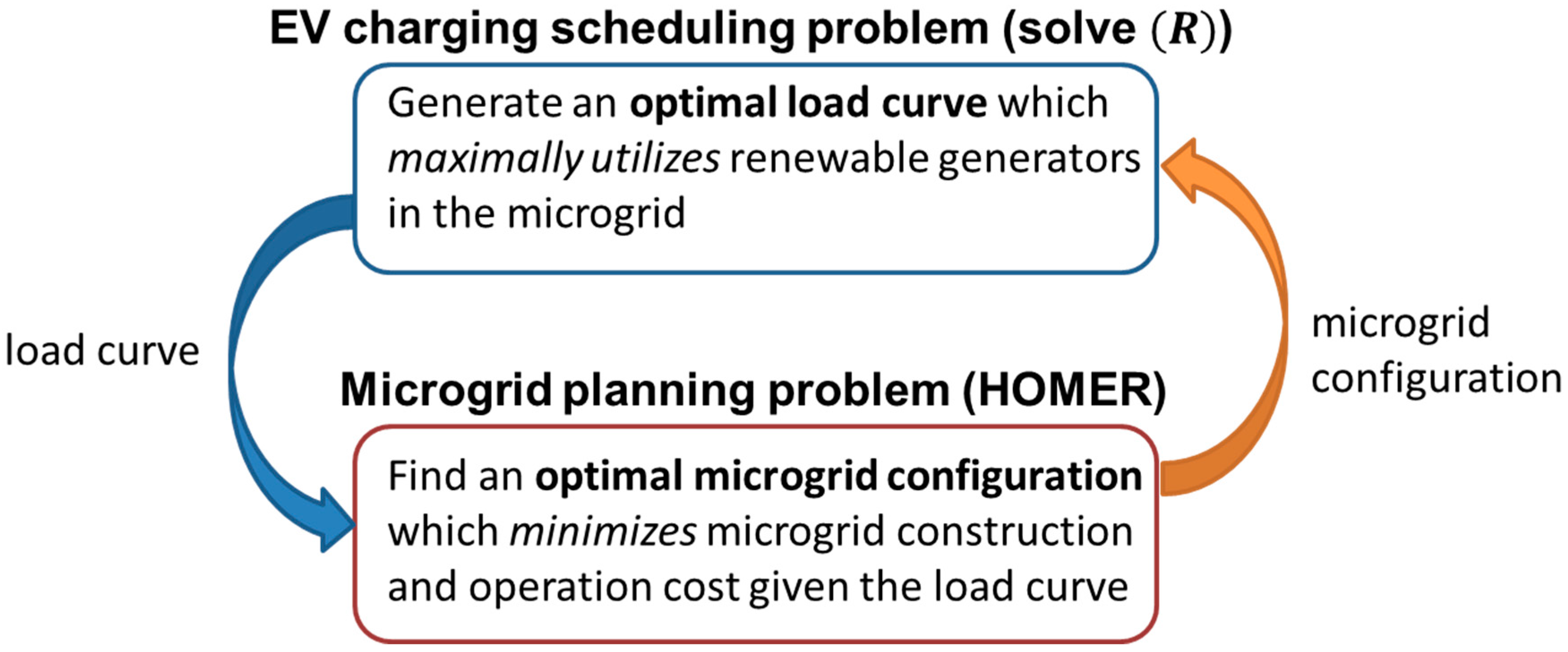
Figure 1 shows the structure of the proposed microgrid planning algorithm. The proposed algorithm iteratively solves between an EV charging scheduling problem and a microgrid planning problem until the solution converges. The EV charging scheduling problem is $(\mathrm{R})$ because the goal of this algorithm is the maximum use of renewables. To solve the first problem, a microgrid configuration is required as input and its output is the load curve in the microgrid. Conversely, the second problem requires the load curve and it finds an optimal microgrid configuration that minimizes the microgrid construction and operation cost. This solution is obtained using HOMER.

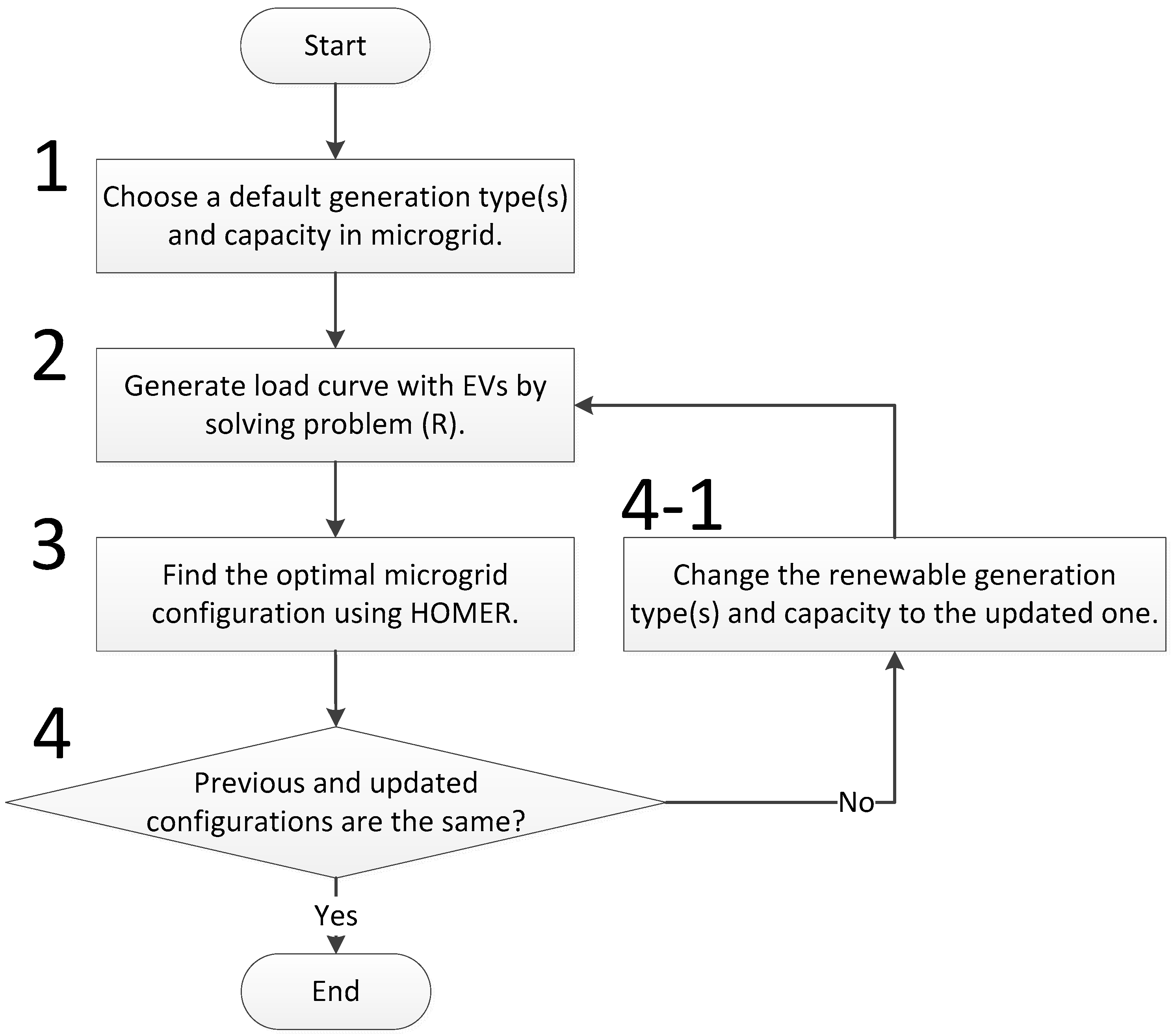
The flowchart of the proposed algorithm is shown in Figure 2, and its explanation is as follows.

Step 1:

The proposed algorithm begins by setting a default renewable generation type(s) and their capacity with given load curve and diverse EV scheduling schemes.

Step 2:

The load curve with EVs using max renewable charging scheme is generated by solving the problem $(\mathrm{R})$ in Section 2.5.

Step 3:

With the updated load curve, the optimal microgrid configuration is investigated using HOMER.

Step 4:

We compare the previous and updated configurations, i.e., generation type and capacity, in the microgrid. If they are the same, the proposed algorithm ends.

Step 4-1: Otherwise, we change the renewable generation types and capacity with the updated ones and the next step is step 2.

In the case study, we use a default setting as the min var scheme’s microgrid configuration. However, any other microgrid configurations can be used as a default. We confirmed that the same final configuration is obtained even if the microgrid configurations with min time and min cost are used as the default setting.

5. Case Study

In this section, two different microgrid cases, i.e., residential microgrid and campus microgrid, are planned at Seoul, Korea. First, the load curves with various EV charging scheduling schemes are presented. Then, optimal microgrid configurations for each load curve are shown.

5.1. Case Study Settings

In this case study, one day is divided into $H=24$ h with the time interval of 1 h.

For EV battery modeling, we use the default parameters of Nissan Leaf [32]. That is, the battery capacity is 24 kWh and ${\delta }_i$ for the residential area, i.e., level 2 charging, is 3.3 kW. Average driving efficiency is 5.36 km/kWh and ${\mu }_c=0.85$.

For an EV $i$, the EV parameters, i.e., arrival time ${\alpha }_i$, departure time ${\beta }_i$, and battery capacity to charge $E_i$, are randomly generated. To obtain the values for these parameters, we use the “2009 National Household Travel Survey” reported by the US Department of Transportation [33]. According to the survey data, the average daily vehicle kilometers of travel is 46.62 km. From the parameters of the Nissan Leaf [32], 10.2 kWh is required to drive 46.62 km. It is then assumed that $E_i/{\mu }_c$, ${\alpha }_i$, and ${\beta }_i$ are uniformly distributed in [8 kWh, 12 kWh], [5 p.m. 9 p.m.], and [5 a.m., 7 a.m.], respectively. Note that the considered arrival and departure time ranges cover more than 90% of drivers [33].

To use the max renewable charging scheme, $E(R^h)$ in the problem $(\mathrm{R})$ is needed. In this case study, no specific distribution for $R^h$ is assumed, but we use real measurement data to get $E(R^h)$. We have the output data of a 30 kW PV generator in Korea. Then, the output of a PV generator in microgrid is interpolated with the measurement data. For example, if a PV generator has 100 kW capacity, its output is obtained by multiplying the measurement data by 3.33.

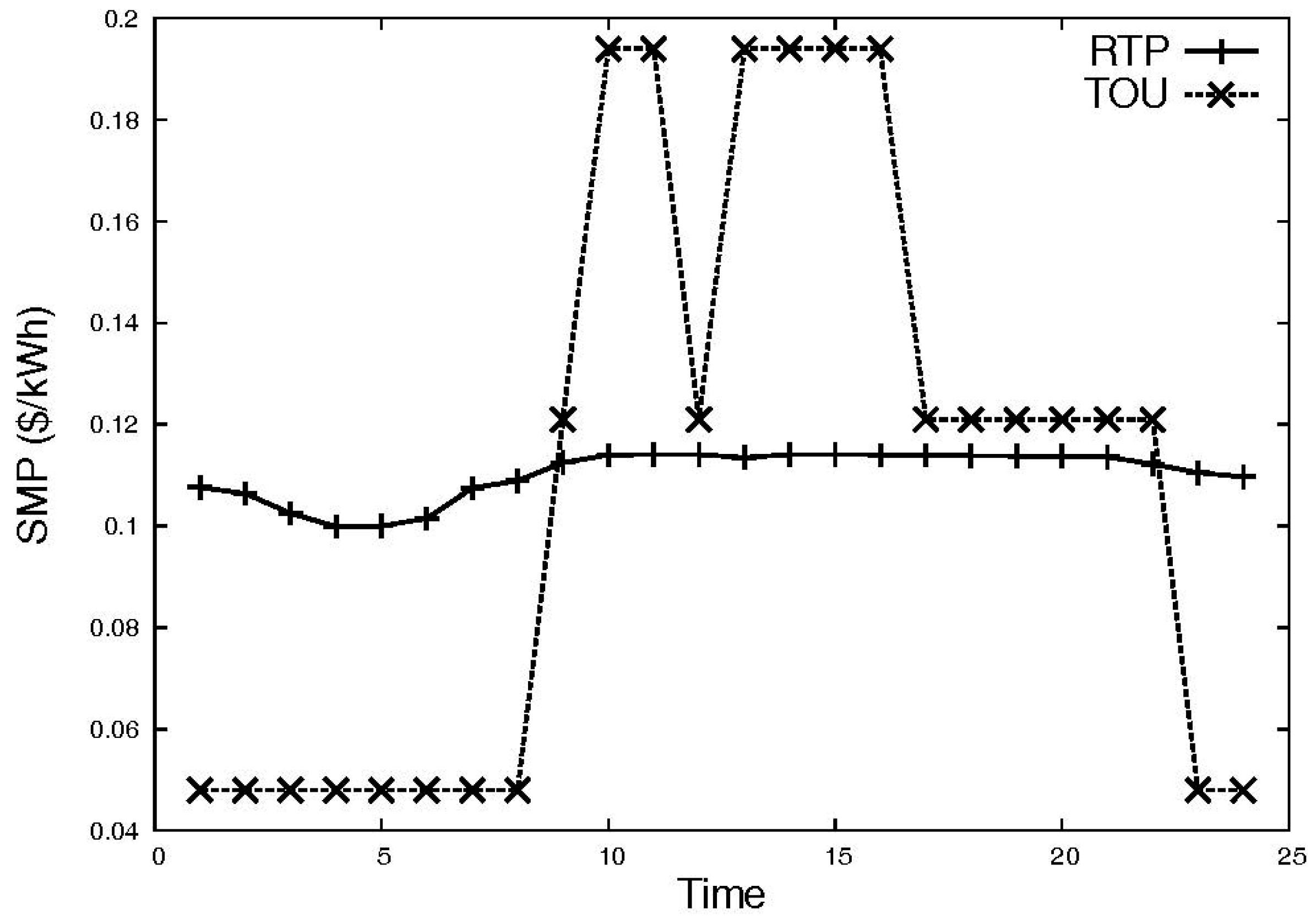
The TOU-based EV charging price rate of KEPCO is used for the min cost1 charging scheme. However, the results of this work are not limited to the KEPCO price rate. Any TOU pricing-based EV charging tariff shows a similar result. For the min cost2, i.e., RTP, it is assumed that the system marginal price (SMP) at each hour is the electricity price for the hour. Figure 3 shows the SMP in summer 2014 obtained by Korea Power Exchange and the TOU-based EV charging price rate. Note that the SMP of a day is announced every day, but the TOU price rate is the same.

5.2. Load Curve with EVs

5.2.1. Residential Area

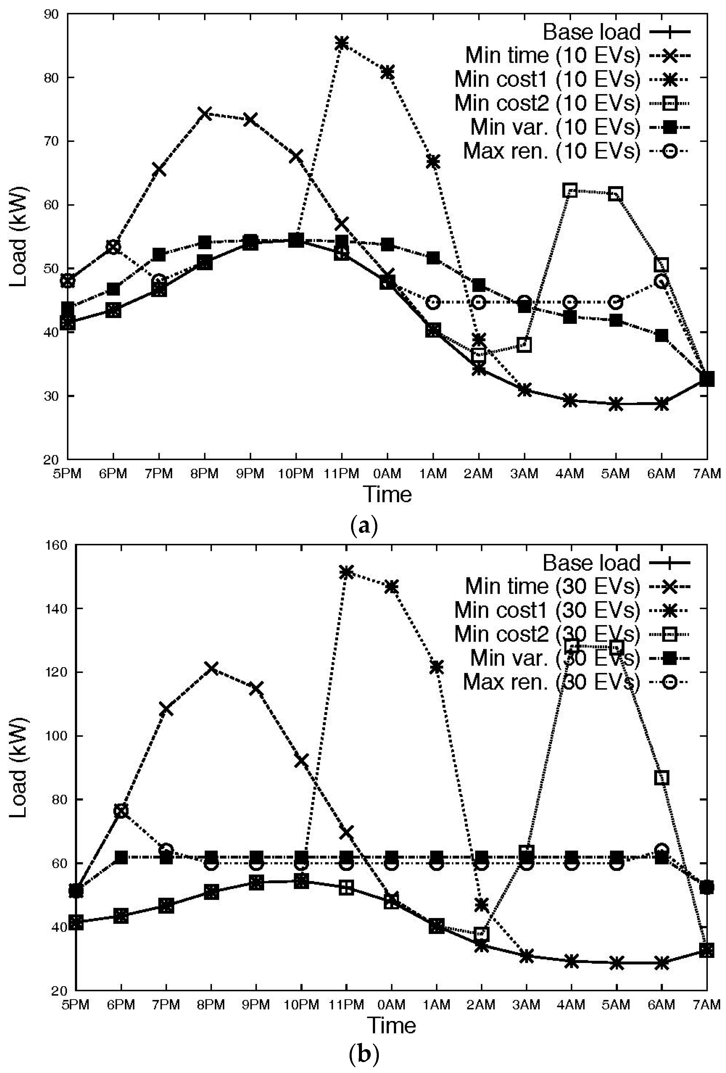
We first consider a microgrid for a residential area with 100 households. A household load curve is obtained from [29]. We use the residential load curve during the summer season, which is shown in Figure 4 as “Base load”. The electricity consumption for one day is 9.85 kWh and the peak demand is 0.54 kW at 10 p.m. With this base load, the EV charging demand is added.

The daily load curve shape changes according to the EV penetration ratio and charging scheduling schemes. Figure 4 shows the load curve for the residential area with the min time, min cost1, min cost2, min Var, and max renewable charging scheduling schemes. We consider 10 EVs and 30 EVs cases, which refer to the EV penetration ratios of 10% and 30%, respectively. Since we assumed that all EVs return home from 5 p.m. to 9 p.m., and leave home from 5 a.m. to 7 a.m. [33], Figure 4 shows only the period when EVs are parked, i.e., from 5 p.m. to 7 a.m. For the uncontrolled charging scheduling schemes, i.e., min time, min cost1, and min cost2 charging schemes, even if a few EVs (2–3 EVs) exist in the residential area, the peak demand and time are changed.

In the case of the min time charging scheme, the charging demands are naturally distributed as the arrival times of EVs are distributed in [5 p.m., 9 p.m.], resulting in less peak demand than that of the min cost schemes. For the min Var charging scheme, the EV charging demand first fills the valley of the off-peak hours. Therefore, the peak demand is not increased to 20 EVs. The max renewable charging scheme shows similar load curve to that of min Var charging scheme, but it reveals two small peak demands at 6 p.m. at 6 a.m. since PV generates power at those times.

Note that in this scenario, only PV generation is considered as the renewable generation since wind speed is insufficient to be competitive.

5.2.2. Campus

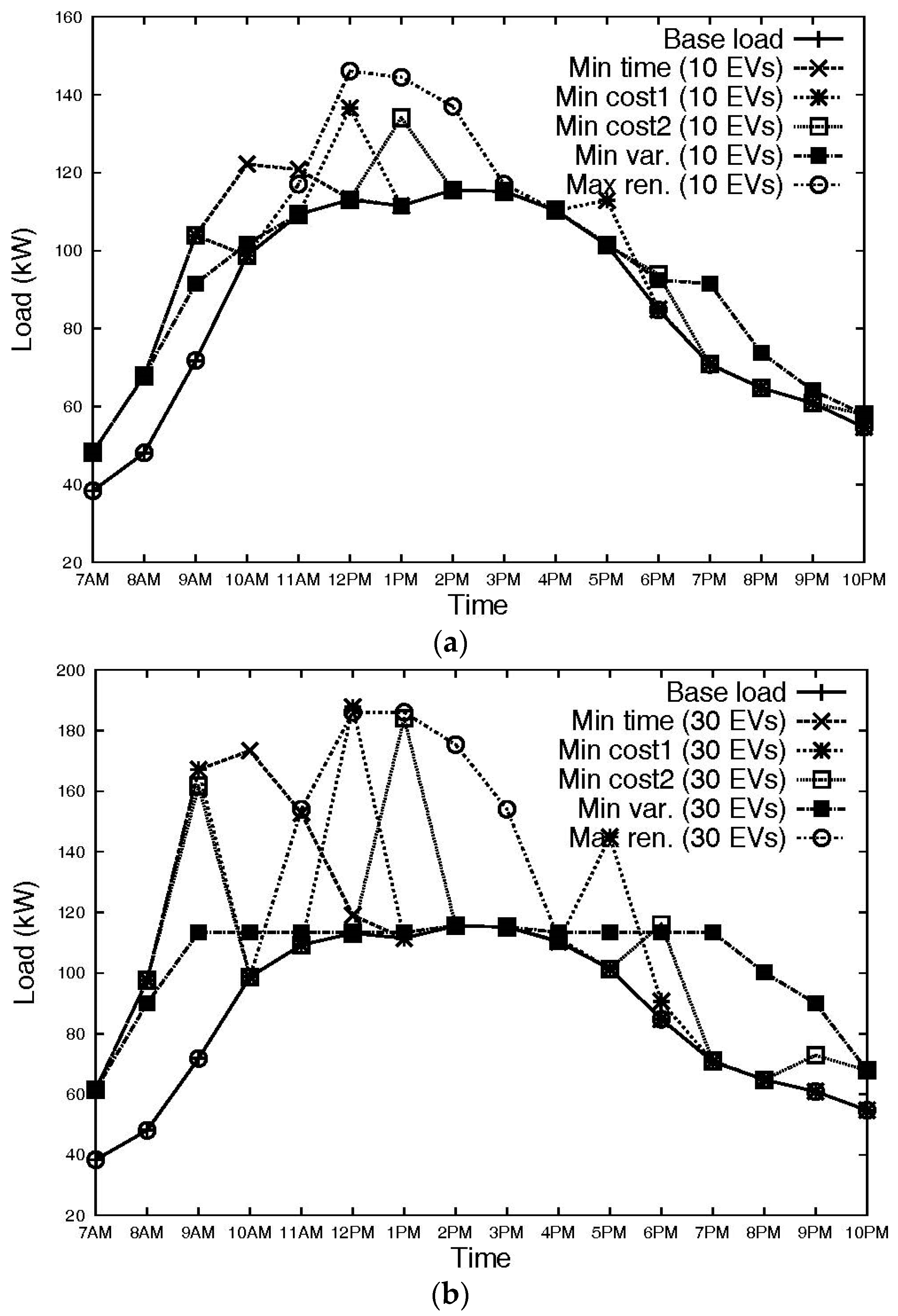
The base load curve for the campus is also obtained from the measurement report in [29]. We use the campus load curve during the summer season, which is shown in Figure 5 as “Base load”. The total electricity consumption for one day is 1687 kWh and the peak demand of 115.6 kW occurred at 2 p.m.

The same average daily vehicle kilometers of travel, ${\alpha }_i$, and ${\beta }_i$ are used with an offset of driving time to work. That is, $E_i/{\mu }_c$, ${\alpha }_i$, and ${\beta }_i$ are uniformly distributed in [8 kWh, 12 kWh], [7 a.m., 9 a.m.], and [5 p.m., 10 p.m.], respectively. In this case, it is assumed that all EVs are charged on the campus. Therefore, Figure 5, which displays the load curve for the campus, shows only the period when EVs are parked at the campus, i.e., from 7 a.m. to 10 p.m.

The min time and min cost charging schemes increase peak demand while the peak demand for the min Var charging scheme is not changed for the 30 EVs. The min cost1 charging scheme has three spikes at 9 a.m., 12 p.m., and 5 p.m. because of the KEPCO EV charging price rate. The second spike is the peak demand since the base load at 12 p.m. is the highest among the three spike times. Similar tendency is shown in the min cost2 charging scheme. The load curve of the max renewable charging scheme shows the same shape as the general PV generation output, and the peak demand of the scheme is the same as those of the min cost charging schemes.

5.3. Optimal Microgrid Planning

With these load curves, the optimal microgrid configurations are obtained using HOMER. In this section, the microgrid operates as the island mode. Section 5.3 discusses the case of the microgrid in grid-connected mode.

5.3.1. Residential Area

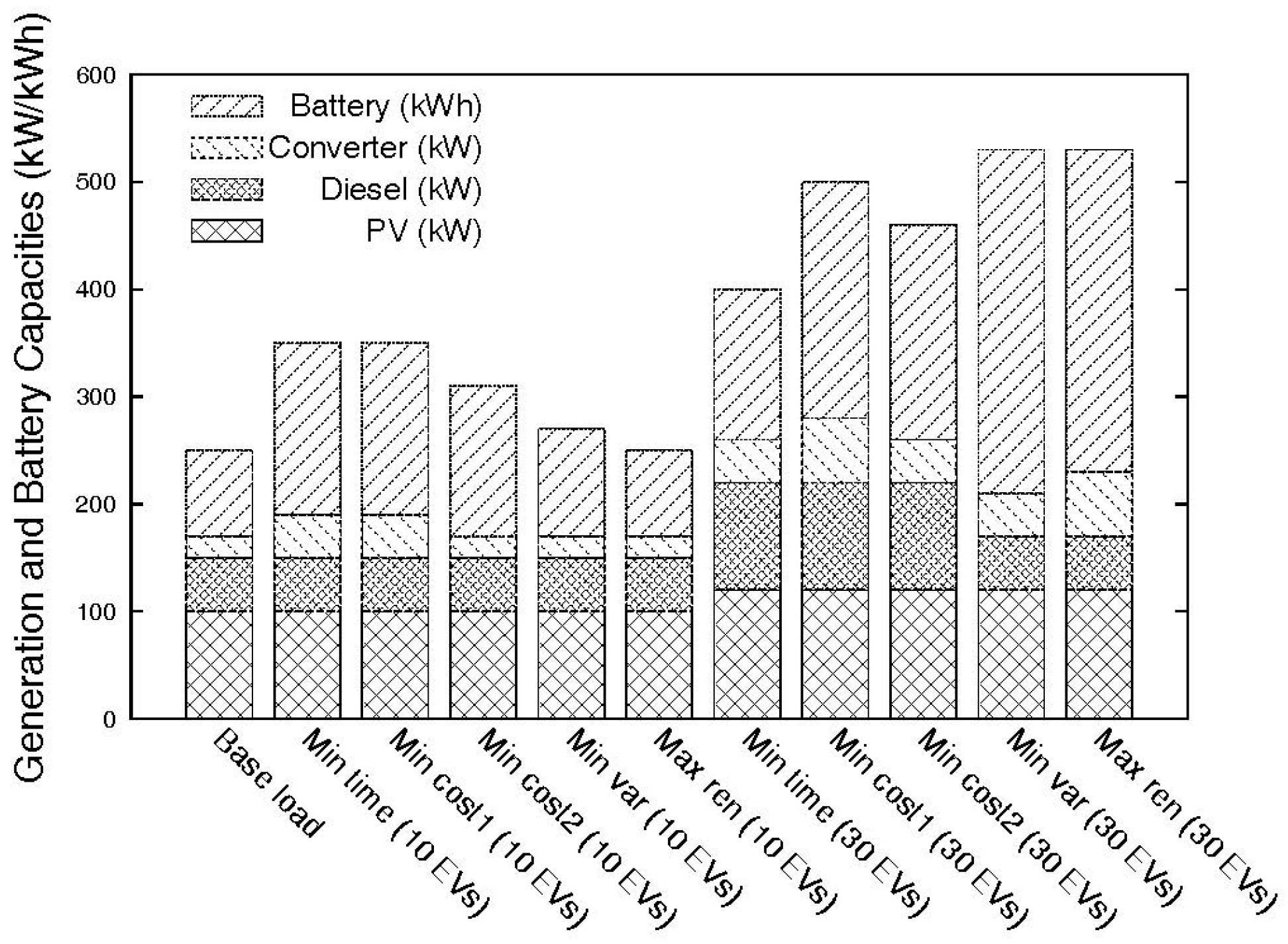
Figure 6 shows the optimal microgrid configurations for the residential area for various EV charging schemes. The microgrid configurations using the min var charging scheme and the proposed algorithm show considerably similar generation and battery capacities (PV and diesel generations) to the base load since load curves show similar shape as shown in Figure 4. Because they only have 50 kW diesel generation capacity with 30 EVs, more battery capacity is required to make a robust microgrid. On the other hand, the other charging schemes have greater diesel generator capacity to support the peak demand in the 30 EVs scenario.

Table 3. Investment cost and CO₂ emission for the residential microgrid configurations.

	Initial Capital ($)	Operating Cost ($/yr)	Total NPC ($)	CO2 Emission (kg/yr)
Base load	355,000	122,169	1,916,725	206,555
Min time (10 EVs)	385,000	144,970	2,238,198	238,495
Min cost1 (10 EVs)	385,000	145,172	2,240,789	237,407
Min cost2 (10 EVs)	373,000	132,456	2,066,238	223,564
Min var. (10 EVs)	361,000	132,744	2,057,912	226,512
Max ren. (10 EVs)	355,000	133,387	2,060,134	229,090
Min time (30 EVs)	464,000	186,050	2,842,343	295,585
Min cost1 (30 EVs)	494,000	200,611	3,058,487	308,342
Min cost2 (30 EVs)	482,000	181,905	2,807,361	285,764
Min var. (30 EVs)	493,000	176,020	2,743,129	279,366
Max ren. (30 EVs)	493,000	175,139	2,731,867	279,578

shows the investment costs and CO₂ emission of the optimal microgrid configurations for each case in detail. The configuration with the min cost1 charging scheduling scheme and the proposed max renewable microgrid configuration are the most expensive and the least expensive solutions to construct the residential microgrid, respectively. The total NPC differences between scheduling schemes are small with 10 EVs, but the gap increases with a number of EVs. The total NPC of the proposed microgrid with 30 EVs saves 10.3% of the cost compared with that of the min cost1 scheme with 30 EVs.

Note that the microgrid with min Var scheme and the proposed microgrid show almost the same result because the PV generation has no impact during the night. In case of the campus microgrid, the two schemes show different results.

5.3.2. Campus

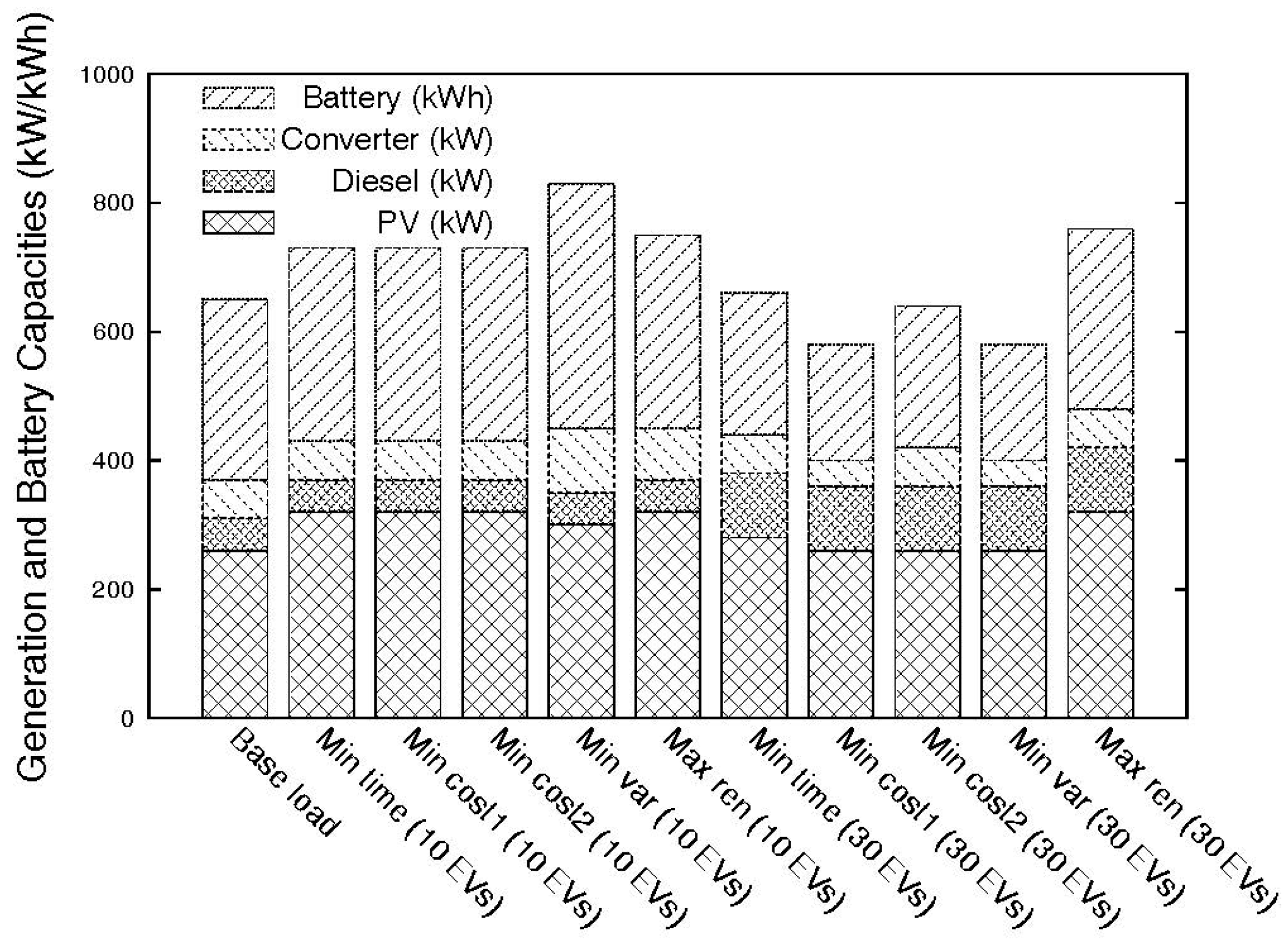
Optimal microgrid configurations for the campus are shown in Figure 7. Unlike the residential microgrid, the configuration for the min Var charging scheme is different to that of the proposed microgrid configuration. Due to the nature of maximizing renewable generation, the proposed microgrid requires the highest renewable capacity.

Table 4. Investment cost and CO₂ emission for the campus microgrid configurations.

	Initial Capital ($)	Operating Cost ($/yr)	Total NPC ($)	CO2 Emission (kg/yr)
Base load	907,000	164,152	3,005,418	267,598
Min time (10 EVs)	1,093,000	164,866	3,200,540	265,982
Min cost1 (10 EVs)	1,093,000	164,926	3,201,313	265,965
Min cost2 (10 EVs)	1,093,000	165,345	3,206,659	266,298
Min var. (10 EVs)	1,069,000	173,858	3,291,483	275,034
Max ren. (10 EVs)	1,099,000	159,638	3,139,714	257,876
Min time (30 EVs)	974,000	211,326	3,675,459	336,167
Min cost1 (30 EVs)	896,000	218,647	3,691,036	352,969
Min cost2 (30 EVs)	914,000	217,554	3,695,074	349,272
Min var. (30 EVs)	896,000	224,112	3,760,900	364,809
Max ren. (30 EVs)	1,112,000	191,039	3,554,125	292,955

shows the investment costs and CO₂ emission for various EV charging schemes in the campus microgrid. The configuration with the min Var charging scheme and the proposed microgrid configuration show the maximum and minimum total NPC, respectively. Again, the cost savings increase with a number of EVs. Since the load curve of the min Var charging scheme shows a flat shape, PV generation is not a viable solution. Therefore, it mainly depends on diesel generation resulting in the highest cost and CO₂ emission. On the other hand, the proposed microgrid maximally utilizes the PV generation output, so it shows the lowest CO₂ emission despite the same diesel generation capacity.

5.4. Discussion

The optimal microgrid configuration in the grid-connected mode is also investigated. When the electricity rate of the main grid is set to SMP as shown in Figure 3, the optimal microgrid configurations for residential and campus are not cost-effective for installing distributed generators. It is because the electricity price of the main grid is lower than installing distributed generators. Therefore, the daily load curve in the grid-connected mode microgrid is “min cost1” or “min cost2” in Figure 3 and Figure 4 according to the pricing schemes.

As shown in Figure 3 and Figure 4, the current EV pricings (TOU pricing and one day before RTP) fail to distribute EV charging load. Therefore, a more intelligent pricing scheme or EV aggregator, which interacts between retailer and EV customer, is required to distribute the EV charging load [34].

In general, a flat load curve reduces investment and O & M cost in the power system. However, when there are many deferrable loads and renewable generations, the flat daily load curve increases the cost. If the deferrable loads follow the outputs of the renewable generation, we can construct a more economical microgrid.

If the microgrid only has diesel generators, the CO₂ emission for residential and campus microgrids are 459,370 kg/yr and 692,302 kg/yr, respectively, in the 30 EVs scenario. That is, the max renewable charging scheme reduces the CO₂ emission as 39.1% and 57.7% in comparison with those of diesel only microgrid. This result achieves the greenhouse gas reduction target of Korea according to the Paris agreement.

The proposed microgrid planning algorithm theoretically provides a configuration that reveals minimum CO₂ emission since it maximally uses renewable generators. In practice, the randomness of renewable generators sometimes causes lower CO₂ emissions by other configurations than the proposed algorithm. However, the difference is minimal, i.e., less than 1%, and this case occurrs when the renewable generators make small contributions as shown in the residential microgrid result. The proposed algorithm results in a significant reduction of CO₂ emissions when renewable generators contribute significantly like in a campus microgrid.

We also considered the wind turbine option, but our configurations do not include wind turbines because wind speed in Seoul, Korea is too low to be a competitive solution [35].

6. Conclusions

To reduce greenhouse gas in the power industry, harmonizing between the two emerging technologies, i.e., microgrid and electric vehicles (EVs) is critical. Therefore, the microgrid planning problem should consider the number of customers in the area who will purchase EVs and how the EV charging loads will be distributed. In this paper, we investigated several uncontrolled and controlled EV charging scheduling schemes: the min time charging scheme, two cost minimization charging schemes, the minimization of variance (min Var) charging scheme, and the max renewable charging scheme. In addition, the optimal microgrid configurations for those charging schemes and different EV penetration ratios were investigated using HOMER. Finally, we proposed a microgrid planning algorithm for a maximum use of renewable generators. The proposed algorithm iteratively solves the EV charging scheduling and microgrid configuration problems to maximally use the renewable generations. Through residential and campus microgrids case studies, the proposed algorithm constructs an economical microgrid with less CO₂ emissions. If the installed renewable generation does not produce output power during EV charging, the proposed algorithm works like the min Var charging scheme. Otherwise, it maximizes the use of renewable generations resulting in the lowest investment cost and CO₂ emission.

References

- UNFCCC. Adoption of the Paris Agreement. Report No. FCCC/CP/2015/L.9/Rev.1 2015. Available online: http://unfccc.int/resource/docs/2015/cop21/eng/l09r01.pdf (accessed on 23 September 2017).
- Trigg, T.; Telleen, P. Global EV Outlook—Understanding the Electric Vehicle Landscape to 2020; International Energy Agency: Paris, France, 2013. [Google Scholar]
- Clement-Nyns, K.; Haesen, E.; Driesen, J. The Impact of Charging Plug-In Hybrid Electric Vehicles on a Residential Distribution Grid. IEEE Trans. Power Syst. 2010, 25, 371–380. [Google Scholar] [CrossRef] [Green Version]
- Kim, J.-H.; Kim, C.-H. Smart EVs Charging Scheme for Load Leveling Considering ToU Price and Actual Data. J. Electr. Eng. Technol. 2017, 12, 1–10. [Google Scholar] [CrossRef]
- Deilami, S.; Masoum, A.; Moses, P.; Masoum, M. Real-Time Coordination of Plug-in Electric Vehicle Charging in Smart Grids to Minimize Power Losses and Improve Voltage Profile. IEEE Trans. Smart Grid 2011, 2, 456–467. [Google Scholar] [CrossRef]
- Sharma, I.; Canizares, C.; Bhattacharya, K. Smart Charging of PEVs Penetrating into Residential Distribution Systems. IEEE Trans. Smart Grid 2014, 5, 1196–1209. [Google Scholar] [CrossRef]
- Tang, W.; Zhang, Y. A Model Predictive Control Approach for Low-Complexity Electric Vehicle Charging Scheduling: Optimality and Scalability. IEEE Trans. Power Syst. 2017, 32, 1050–1063. [Google Scholar] [CrossRef]
- Hu, J.; You, S.; Lind, M.; Østergaard, J. Coordinated Charging of Electric Vehicles for Congestion Prevention in the Distribution Grid. IEEE Trans. Smart Grid 2014, 5, 703–711. [Google Scholar] [CrossRef] [Green Version]
- Yoon, S.-G.; Choi, Y.-J.; Park, J.-K.; Bahk, S. Stackelberg Game based Demand Response for at-Home Electric Vehicle Charging. IEEE Trans. Veh. Technol. 2016, 65, 4172–4184. [Google Scholar] [CrossRef]
- Gan, L.; Topcu, U.; Low, S. Optimal Decentralized Protocol for Electric Vehicle Charging. IEEE Trans. Power Syst. 2013, 28, 940–951. [Google Scholar] [CrossRef]
- Sun, B.; Huang, Z.; Tan, X.; Tsang, D. Optimal Scheduling for Electric Vehicle Charging with Discrete Charging Levels in Distribution Grid. IEEE Trans. Smart Grid 2016. [Google Scholar] [CrossRef]
- Venkataramanan, G.; Marnay, C. A Larger Role for Microgrids. IEEE Power Energy Mag. 2008, 6, 78–82. [Google Scholar] [CrossRef]
- Kwasinski, A.; Krishnamurthy, V.; Song, J.; Sharma, R. Availability Evaluation of Micro-Grids for Resistant Power Supply during Natural Disasters. IEEE Trans. Smart Grid 2012, 3, 2007–2018. [Google Scholar] [CrossRef]
- Wu, T.; Yang, Q.; Bao, Z.; Yan, W. Coordinated Energy Dispatching in Microgrid with Wind Power Generation and Plug-in Electric Vehicles. IEEE Trans. Smart Grid 2013, 4, 1453–1463. [Google Scholar] [CrossRef]
- Jian, L.; Xue, H.; Xu, G.; Zhu, X.; Zhao, D.; Shao, Z. Regulated Charging of Plug-in Hybrid Electric Vehicles for Minimizing Load Variance in Household Smart Microgrid. IEEE Trans. Ind. Electron. 2013, 60, 3218–3226. [Google Scholar] [CrossRef]
- Hafez, O.; Bhattacharya, K. Optimal Planning and Design of a Renewable Energy Based Supply System for Microgrids. Renew. Energy 2012, 45, 7–15. [Google Scholar] [CrossRef]
- Stadler, M.; Marnay, C.; DeForest, N.; Eto, J.; Cardoso, G.; Klapp, D.; Lai, J. Web-Based Economic and Environmental Optimization of Microgrids. In Proceedings of the IEEE Innovative Smart Grid Technologies (ISGT), Washington, DC, USA, 16–20 January 2012. [Google Scholar]
- Khodaei, A.; Bahramirad, S.; Shahidehpour, M. Microgrid Planning under Uncertainty. IEEE Trans. Power Syst. 2015, 30, 2417–2425. [Google Scholar] [CrossRef]
- Khodaei, A. Provisional Microgrid Planning. IEEE Trans. Smart Grid 2017, 8, 1096–1104. [Google Scholar] [CrossRef]
- Narayan, A.; Ponnambalam, K. Risk-Averse Stochastic Programming Approach for Microgrid Planning under Uncertainty. Renew. Energy 2017, 101, 399–408. [Google Scholar] [CrossRef]
- Richardson, P.; Flynn, D.; Keane, A. Optimal Charging of Electric Vehicles in Low-Voltage Distribution Systems. IEEE Trans. Power Syst. 2012, 27, 268–279. [Google Scholar] [CrossRef]
- Electric Vehicle (EV) Rate Plans, PG&E. Available online: https://www.pge.com/en_US/residential/rate-plans/rate-plan-options/electric-vehicle-base-plan/electric-vehicle-base-plan.page (accessed on 22 August 2017).
- Electric Rates Table, KEPCO. Available online: http://cyber.kepco.co.kr/ckepco/front/jsp/CY/E/E/CYEEHP00202.jsp (accessed on 22 August 2017).
- Acha, S.; Green, T.; Shah, N. Optimal Charging Strategies of Electric Vehicles in the UK Power Market. In Proceedings of the IEEE Innovative Smart Grid Technologies (ISGT), Anaheim, CA, USA, 17–19 January 2011. [Google Scholar]
- HOMER Energy. Available online: http://www.homerenergy.com/ (accessed on 27 July 2017).
- Net Present Value. Wikipedia. Available online: https://en.wikipedia.org/wiki/Net_present_value (accessed on 27 July 2017).
- Lambert, T.; Gilman, P.; Lilienthal, P. Micropower System Modeling with HOMER. In Integration of Alternative Sources of Energy; Farret, F., Simões, M., Eds.; John Wiley & Sons: Hoboken, NJ, USA, 2006. [Google Scholar]
- South Australian Government, Data Collection of Diesel Generators in South Australia, September 2013. Available online: http://www.renewablessa.sa.gov.au/investor-information/diesel-generators-directory (accessed on 27 July 2017).
- Korea Energy Agency, Electrical Consumption Pattern Analysis by using the Customer Load Curve, March 2007. Available online: http://www.kemco.or.kr/web/kem_home_new/info/data/open/kem_view.asp?sch_key=&sch_value=&sch_cat=&c=306&q=12847 (accessed on 27 July 2017).
- NASA Surface Meteorology and Solar Energy Website. Available online: https://eosweb.larc.nasa.gov/sse/ (accessed on 27 July 2017).
- Diesel Prices. Available online: http://www.globalpetrolprices.com/diesel_prices/ (accessed on 27 July 2017).
- Nissan Leaf. Available online: https://www.nissanusa.com/electric-hybrid-cars (accessed on 27 July 2017).
- Summary of Travel Trends: 2009 National Household Travel Survey. Available online: http://nhts.ornl.gov/ (accessed on 27 July 2017).
- Ortega-Vazquez, M.; Bouffard, F.; Silva, V. Electric Vehicle Aggregator/System Operator Coordination for Charging Scheduling and Services Procurement. IEEE Trans. Power Syst. 2013, 28, 1806–1815. [Google Scholar] [CrossRef]
- Korea Meteorology Administration Website. Available online: http://www.kma.go.kr/ (accessed on 27 July 2017).
- Boyd, S.; Vandenberghe, L. Convex Optimization; Cambridge University Press: Cambridge, UK, 2004. [Google Scholar]
- Grant, M.; Boyd, S. CVX: Matlab Software for Disciplined Convex Programming, Version 1.22. Available online: http://cvxr.com/cvx (accessed on 27 July 2017).
Figure 1.
Structure of the proposed microgrid planning algorithm.
Figure 2.
Flowchart for the proposed microgrid planning algorithm.
Figure 3.
Daily system marginal price (SMP) in summer 2014 in Korea and TOU-based EV charging price rate.
Figure 4.
Load curves from 5 p.m. to 7 a.m. for the residential area. (a) 10 EVs; (b) 30 EVs.
Figure 5.
Load curves from 7 a.m. to 10 p.m. for the campus. (a) 10 EVs; (b) 30 EVs.
Figure 6.
Optimal microgrid configurations for the residential area.