PV Hosting Capacity Analysis and Enhancement Using High Resolution Stochastic Modeling

Abstract

Reduction of CO₂ emissions is a main target in the future smart grid. This goal is boosting the installation of renewable energy resources (RES), as well as a major consumer engagement that seeks for a more efficient utilization of these resources toward the figure of ‘prosumers’. Nevertheless, these resources present an intermittent nature, which requires the presence of an energy storage system and an energy management system (EMS) to ensure an uninterrupted power supply. Moreover, network-related issues might arise due to the increasing power of renewable resources installed in the grid, the storage systems also being capable of contributing to the network stability. However, to assess these future scenarios and test the control strategies, a simulation system is needed. The aim of this paper is to analyze the interaction between residential consumers with high penetration of PV generation and distributed storage and the grid by means of a high temporal resolution simulation scenario based on a stochastic residential load model and PV production records. Results of the model are presented for different PV power rates and storage capacities, as well as a two-level charging strategy as a mechanism for increasing the hosting capacity (HC) of the network.

1. Introduction

Electrical energy is one of the main elements for the development of modern society, where higher quality and reliability are requested by the consumers whilst reducing emissions and increasing efficiency. In the current context, this has led to the integration of large renewable resources in the electrical grid, meaning a high percentage of the total production in many countries. In the European Union (UE), renewable energies represented 25.4% of the total primary energy production in 2015, and among these sources, solar energy accounted for 4.17% of the total annual renewable production [1].

Nevertheless, the variability and uncertainty associated with these types of sources prevent them from taking part in the electricity market, due to their low dispatchability and the perturbations that they might cause in the grid [2]. Therefore, the effective management of these resources is one of the current challenges, usually solved by means of electrical storage systems [3]. However, storage systems have a considerable cost, and they must be combined with advanced control strategies that maximize their utilization without negatively impacting the lifespan [4].

Opposed to the classical unidirectional grid conception where the end user is simply a consumer, the new context of distributed resources integration is leading towards the major participation of users, who have acquired the role of ‘prosumers’ that might interact bi-directionally with the electrical network [5]. This change has been promoted thanks to the use of advanced metering infrastructures (AMI), advanced communications and demand response (DR) programs [6,7]. Those programs, despite causing sometimes discomfort, may represent substantial economic and energetic savings [8].

Therefore, users are provided with energy management systems (EMS) that ensure the network stability and an uninterrupted supply, all of these by controlling the charging cycles, as well as the possible interactions with the main grid when either an energy surplus or shortage take place [9]. Likewise, this interaction with the grid might contribute to the improvement of the network stability by means of the intercommunication between EMSs. This is particularly useful in decentralized installations or communities with a distributed generation where a global smart community energy management system (SCEMS) is needed to avoid an uncontrolled energy injection that might lead to the overload of the network, exceeding the so-called hosting capacity (HC) [10,11].

In order to assess the future scenarios and develop effective control strategies that overcome these issues, simulation systems are highlighted as an essential tool. Between all the different alternatives, those modeling techniques that provide a high-temporal resolution are regarded as the most suitable ones due to the random nature of the end users’ consumption and the renewable sources [12,13].

In this context, stochastic models can be pointed out as the main tools for high temporal resolution simulations since they are able to emulate the chaotic consumers’ behavior whilst keeping the aggregate trend. A wide range of previous works can be found in the literature regarding these models. In [14,15], Widen et al. modeled the electricity and hot water demand of Swedish households using a bottom-up methodology. Likewise, Richardson et al. developed various models to simulate the residential lighting consumption [16] and the appliances demand [17]. In addition, Mckenna and Thomson [18] implemented the simulation of heating consumption in terms of hot water demand. What is more, the authors have previously developed various models based on the active occupancy, which are able to simulate the lighting [19], appliances andheating, ventilation and air conditioning (HVAC) systems’ consumption [20].

Together with the consumption simulation, the estimation of the instantaneous power produced by the RES must also be done with a high-temporal resolution in order to study the interplay between both elements. In the particular case of PV power, previous authors have based their works on the modeling of irradiance components by means of historical records [21]. Nevertheless, in addition to the global irradiance, some other factors highly influence the PV production such as the technology, the degradation of the components, the energy losses of the installation, the inverters’ performance, etc. [22,23]. In this way, and taking into account the wide available amount of historical records of domestic PV installations and large solar fields, the use of these logs as the main input for the evaluation of future scenarios is one of the most accurate and realistic alternatives [24].

Using this consumption model together with the production records, different scenarios that represent a future grid or installation can be assessed to plan the electrical network, introduce energy management strategies or develop new algorithms. However, it is also necessary to introduce a series of indicators that take into account this high temporal resolution. Previous authors have proposed different quantifiers of the interplay between demand and production such as Sartori et al. [25] and Salom et al. [26], especially in the context of net-zero energy buildings and production-consumption matching. Nevertheless, no additional indicators have been developed to study the integration of distributed energy production in a grid with limited HC.

Therefore, this paper aims to implement a simulation system that allows assessing the integration of PV production and energy storage in a residential context, with a high temporal resolution (1 min) and taking into account the interaction with the grid and the limitations in terms of injected power. Moreover, an indicator of the network interaction with limited HC is introduced, finally, proposing a mechanism for using the distributed storage from the distribution system operator (DSO) point of view to avoid the network overload and enhance the HC in the peak production hours.

The paper is structured as follows. Section 2 presents the main parts of the system and the methodology used to model them, the control strategies, the developed indexes for quantifying the integration and the simulation process. Subsequently, the results obtained using the system are presented in Section 3, first showing the novel characteristics of this simulation system and, posteriorly, evaluating three different scenarios, islanded, grid-connected and grid-connected with HC enhancement operation. Finally, the conclusions are addressed in Section 4.

2. Methodology

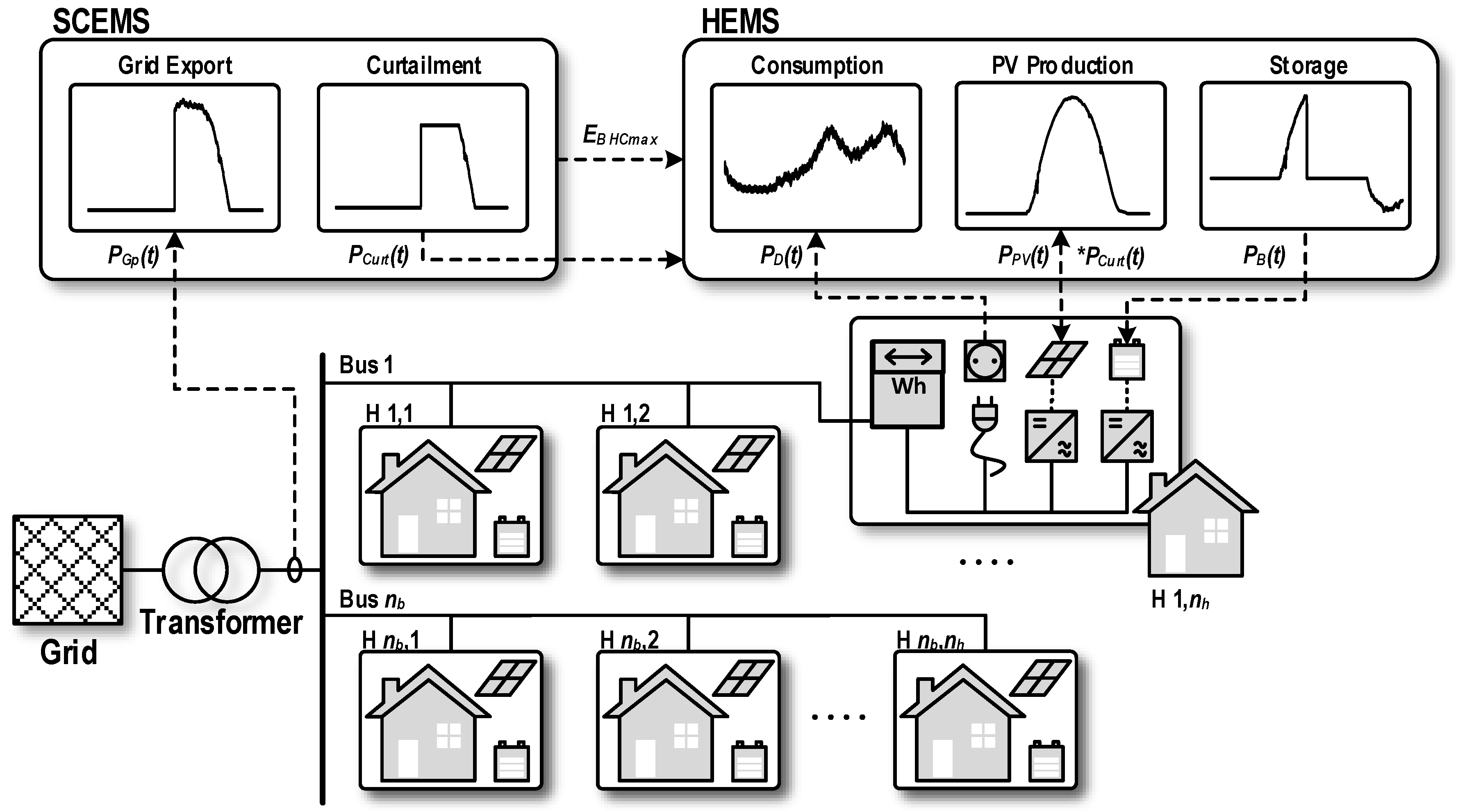
The simulation system aims to represent a low voltage grid composed of $n_h$ households that have distributed renewable production and energy storage systems. Each household is connected to a low-voltage bus $n_b$ that is simultaneously interfaced with the main grid through a medium voltage/low voltage (MV/LV) transformer. The system architecture is shown in Figure 1.

The AC loads are responsible for the power consumption ($P_D\left(t\right)$), and their behavior is modeled by means of a stochastic model. Regarding the PV production ($P_{PV}\left(t\right)$), the panels are considered to be connected through a unidirectional DC/AC converter to the household network. In the case of the batteries ($P_B\left(t\right)$), the converter is bi-directional, so they can interact with the production, as well as with the grid, aiding in the HC process. Moreover, each house is supposed to have a bi-directional smart electricity meter that quantifies the energy flow to and from the grid and sends information to the home EMS (HEMS) and the SCEMS that control the power interchanged with the grid ($P_{Gp}\left(t\right)$) and establish the production curtailments ($P_{Curt}\left(t\right)$) when needed.

The HEMS controls the charging/discharging process of each battery in each household taking into account only the local PV production and the instantaneous consumption. On the top of that, the SCEMS possesses global information about the network status in order to guarantee the stability of the grid and perform the HC enhancement actions when needed using a percentage of the distributed batteries in each dwelling ($E_{BHCMax}$) and reducing the PV production homogeneously between the households ($\ast P_{Curt}\left(t\right)$), according to the curtailment, to avoid the network overcharge.

2.1. Households Simulation

As can be seen in Figure 1, the households are composed of three modeling blocks, which are the AC loads, the PV production and the energy storage system. The characteristics, modeling methodology and simulation of each system are described below.

2.1.1. AC Load

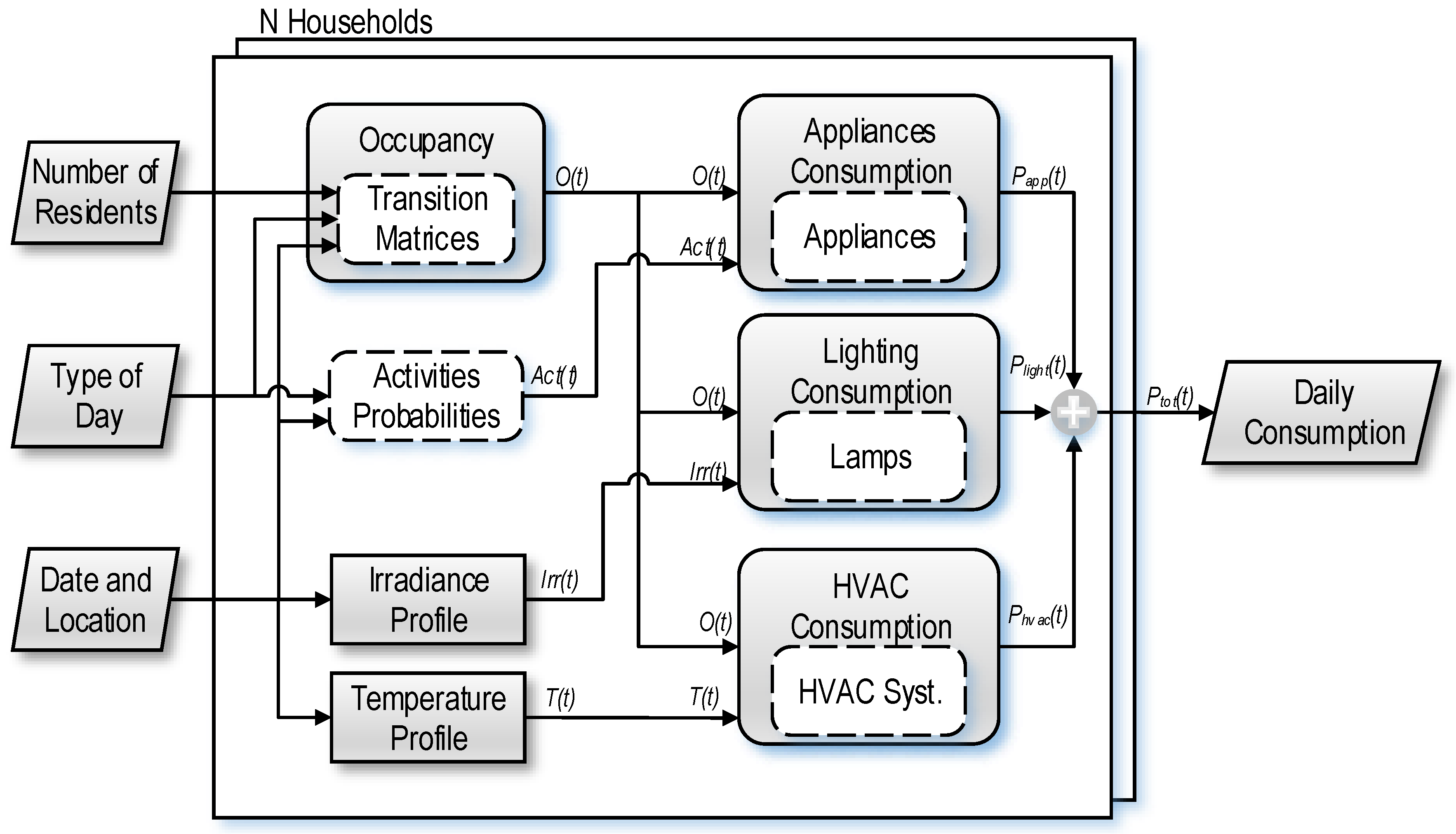
The consumption profiles of each household were calculated using a stochastic model. The estimation uses Monte Carlo simulation techniques and it is based on Markov chains probability theory. The model is composed of four algorithmic blocks that estimate, first, the daily occupancy profiles and, subsequently, the lighting system demand, the consumption due to general home appliances and the needs of HVAC systems, respectively. The general structure of this model is illustrated in Figure 2.

As can be observed, the residents’ behavior is the common influence factor since the activity of the users at home determines the periods when the higher consumption takes place. Thus, the calculation of the daily occupancy profile is the lower level block of the system, denoted as Occupancy in Figure 2. The model has three inputs parameters, which are the number of residents of the household, the type of day (weekday or weekend) and the date and location.

The occupancy model is based on non-homogeneous Markov Chains and has a 10-min resolution. Therefore, for each 10-min interval (144 in a day), the probability transition matrices were calculated. For this aim, the Time Use Survey (TUS) was employed [27]. This survey has been carried out in most European countries, and includes information regarding the interviewees’ activities during the day, where these activities took place and whether the interviewees were accompanied. These matrices determine the different transitions between occupancy states based on a random sampling over the associated discrete probability distribution for a given time and the current state of occupancy [28,29].

Above this block, and using the generated occupancy profile $O\left(t\right)$ as an input dataset, the power demand was calculated applying the three other blocks, each one with specific influence factors and with 1-min resolution. This higher temporal resolution in the consumption patterns is fully justified since, whereas the occupancy transitions occur within a longer interval, being unlikely to have occupancy transitions below 10–15 min, the on/off events of appliances are faster.

From the consumption blocks, the lighting demand block (Lighting Consumption) is influenced by the solar irradiance profile $Irr\left(t\right)$, which determines when the home lighting system are likely to be used. This profile is combined with the occupancy $O\left(t\right)$, so the higher the occupancy level, the higher the probability of switching on the lighting systems when no daylight is available. In addition, by means of a probability distribution of lighting technologies and powers, the lamps that are installed in the household are randomly selected. Further details regarding this model can be found in a previous work [19].

In the case of the appliances consumption block (Appliances Consumption), besides the occupancy profile, the daily probability for different activities $Act\left(t\right)$ was taken into account. These activities were also extracted from the TUS [27], and they are: doing the laundry, ironing, cleaning the house, watching the TV, washing and dressing, cooking and using the PC [29]. Those activities are directly or indirectly related to some energy consumption and subsequently with the probability of turning on the associated appliances. For instance, ironing is directly linked to the use of an iron, whereas the activity cooking can be related to a microwave, an oven or an electric stove.

Finally, the block that estimates the HVAC consumption (HVAC Consumption) uses the annual seasonality and the daily ambient temperature profiles $T\left(t\right)$ as influence factors. The first one relates the energy intensity consumption of each day with the temperature deviation from the comfort one [30] using the regression methodology proposed by Moral-Carcedo and Vicéns-Otero [31], whereas the daily temperature regulates the cycling of the appliances during the day according to the insulation and the devices technology [32]. It should be pointed out that only the electrical demand was studied. Consequently, only those heating appliances supplied with electricity were considered.

The daily consumption profile $P_{tot}\left(t\right)$ for each household n is finally calculated as the sum of the appliances consumption $P_{app}\left(t\right)$, the lighting consumption $P_{light}\left(t\right)$ and the HVAC consumption $P_{HVAC}\left(t\right)$. This confers the model an additional flexibility since not only the global consumption can be studied, but also a specific component can be separated and disaggregated from the rest.

2.1.2. Battery Storage

As was indicated in Figure 1, each household has an energy storage system. A simplified battery model was selected for the study. Its basic operation is ruled by Equation (1).

$$E_B\left(t\right)=\left\{\begin{array}{cc}{E}_B(t-1)+\frac{P_B\left(t\right)}{60}·{\eta }_c\hfill & P_B\left(t\right)\ge 0\hfill \\ E_B(t-1)+\frac{P_B\left(t\right)}{60}·\frac{1}{{\eta }_d}\hfill & P_B\left(t\right)<0\hfill \end{array}\right.$$

(1)

In this equation t represents the simulation time in minutes, $E_B\left(t\right)$ is the stored energy for each simulation step in Wh and $P_B\left(t\right)$ is the instant power applied to (+ charging) or supplied by (− discharging) the storage system for a given time in Watts. The process has an associated charge efficiency ${\eta }_c$ and a discharge efficiency ${\eta }_d$, which depend on the storage technology and can be provided as input parameters. For this study, since no specific storage technology was selected a 0.85 charging and discharging efficiency was assumed. In addition, the energy $E_B\left(t\right)$ is measured in Wh, whereas the instant power is calculated for each minute, so the $1/60$ factor was included.

The stored energy is also limited by the operative range that is expressed in (2). In this equation, $E_{Bmin}$ is the depth of discharge and $E_{Bmax}$ is the charging threshold. These limits are established by the technology of the battery and the selected operation.

$$E_{Bmin}<E_B\left(t\right)<E_{Bmax}$$

(2)

2.1.3. PV Production

The photovoltaic production was emulated using historical records of a rooftop PV installation located in Cordova (Córdoba), Spain, during 3 years, from 2011–2013. The studied system is composed of 3 similar sectors, each of them containing 36 solar modules. The peak power of each module is 165 W, resulting in a total of 5940 W per sector.

At the same time, each sector is associated with an inverter of 5000 W. The inverter is capable of monitoring parameters such as the input DC voltage ($V_{DC}$) and DC current ($I_{DC}$), output AC voltage ($V_{AC}$) and AC current ($I_{AC}$), frequency (f) and power ($P_{PV}$). In addition, a calibrated cell measures the tilted global irradiance ($Irr\left(t\right)$) that is collected by the modules. All of these magnitude are recorded with a 5-min resolution [23].

$$P_{PV}\left(t\right)={\eta }_{inv}·{\eta }_{inst}·{\eta }_G·Irr\left(t\right)$$

(3)

The final production of the PV installation is influenced by a wide range of factors. As indicated in (3), the final power $P_{PV}\left(t\right)$ produced by the PV installation for a given irradiance $Irr\left(t\right)$ mainly depends on the efficiency of the inverter (${\eta }_{inv}$), the installation (${\eta }_{inst}$), meaning wiring losses, diodes losses and inhomogeneous irradiance, and the generator (${\eta }_G$). In order to take into account all of these elements, the output AC power recorded by the inverters was used in the simulations.

$$P_{PV}^{peak}\left(t\right|P_{peak})=\frac{P_{peak}}{P_{peak}^{\ast }}·P_{PV}\left(t\right)$$

(4)

Using the expression indicated in (4) the output AC power $P_{PV}\left(t\right)$ was linearly scaled using the quotient between the selected PV peak per household $P_{peak}$ and the original installation peak $P_{peak}^{\ast }=5940$ W, obtaining the scaled curve $P_{PV}^{peak}$, which is used as the input for the simulation. In addition, the power profiles were linearly interpolated to achieve a 1-min resolution from the original 5-min records. Taking into account the 1-min resolution of the consumption profile, this interpolation does not imply a significant error since large power gradients are mainly associated with events slower than 5 min usually associated with large clouds’ shading, although fast-moving clouds and scattered skies might cause faster variations.

2.2. Hosting Capacity

The HC is defined as the amount of renewable energy that can be integrated into the existing electrical grid without impacting the reliability, quality or performance of the network. The variation of these parameters is studied by means of a series of indicators that must remain between a given threshold such as the voltage, the frequency or the current injected into the grid.

For low voltage grids, the main phenomena that limit the HC of the network are overvoltages and overloads in the system. The first one appears due to the higher R/X (resistance to reactance) radio in low-voltage grids, which might lead to overvoltages when a large amount of current is injected. Nevertheless, the detection of this type of event requires detailed knowledge of the particular network, and its influence is usually small thanks to the oversize of the feeders [33].

On the other hand, the network overload is a more common phenomenon since the distribution transformers are designed to cope with users’ demand, but not with the uncontrolled injection of renewable production into the grid. This leads to the overload of the MV/LV transformers whose protections are usually very slow. Subsequently, as proposed by Etherden and Bollen [10], a coordinated curtailment strategy has to be developed.

In this paper, the phenomenon of the HC was analyzed in the context of the system overload, directly relating the issue with the power ratio of MV/LV transformer represented in Figure 1, which limits the maximum instantaneous power that can be handled. This power can be imposed by the network protections, the capacity of the electrical conductors or even the DSO. Moreover, it might be defined with different levels of reliability and hysteresis ranges.

Two different control schemes in order to reduce the impact of large distributed energy resources’ integration without reinforcing the grid were studied. The so-called soft curtailment and hard curtailment strategies, proposed by Etherden and Bollen [10], were analyzed in this work. These strategies were implemented by the Equations (5) and (6).

$$P_{G_{soft}}\left(t\right)=\left\{\begin{array}{cc}{P}_{Gp}\left(t\right)\hfill & P_{Gp}\left(t\right)<P_{Curt}\hfill \\ P_{Curt}\hfill & P_{Gp}\left(t\right)\ge P_{Curt}\hfill \end{array}\right.$$

(5)

$$P_{G_{hard}}\left(t\right)=\left\{\begin{array}{cc}{P}_{Gp}\left(t\right)\hfill & P_{Gp}\left(t\right)<P_{Curt}\hfill \\ 0\hfill & P_{Gp}\left(t\right)\ge P_{Curt}\hfill \end{array}\right.$$

(6)

In these two equations, $P_{Gp}\left(t\right)$ is the instantaneous aggregate PV power injected by the smart community, whereas $P_{Curt}$ is the maximum power flow allowed through the MV/LV transformer. In addition, $P_{G_{soft}}\left(t\right)$ and $P_{G_{hard}}\left(t\right)$ indicate the real power injected into the grid when either soft or hard curtailment strategies respectively are applied.

As can be derived from (5) and (6), the strategies differ in the amount of power that is allowed to be injected into the grid when a potential overload is detected. The soft curtailment represents the most favorable case, whereas the hard curtailment is the worst case scenario. Within these two strategies, a wide range of alternatives can be chosen with different levels of coordination.

In the case of soft curtailment, the system has enough control capabilities, so the power exported is limited to the maximum power ratio. This situation is completely feasible in the study case, since the distributed PV production units can be selectively disconnected for this aim.

On the other hand, when a hard curtailment is applied, the entire power injection is disconnected under an overload situation. This strategy requires lower control capabilities in the system, but the amount of energy that is exported is also dramatically decreased. For our study, since a 200-household community was studied, considering an average 2000 W consumption per house, the power ratio of the transformer $P_{Curt}$ was selected to be 400,000 VA.

2.3. Smart Community Energy Management System

The last block of the simulation is the SCEMS that controls the power interchange between the different units and implements the above-mentioned curtailment strategies.

2.3.1. EMS: Self-Consumption Maximization

The EMS in each household aims to maximize the autonomy of the dwelling. Therefore, the distributed storage is charged as soon as the PV production exceeds the consumption to accumulate energy for the non-production period. Once the batteries are fully charged, the production surplus is injected into the grid considering the HC limits. Finally, when the available PV production is too low, the demand is supplied by the batteries until they are discharged, and then, the demand has to be covered by importing energy from the grid.

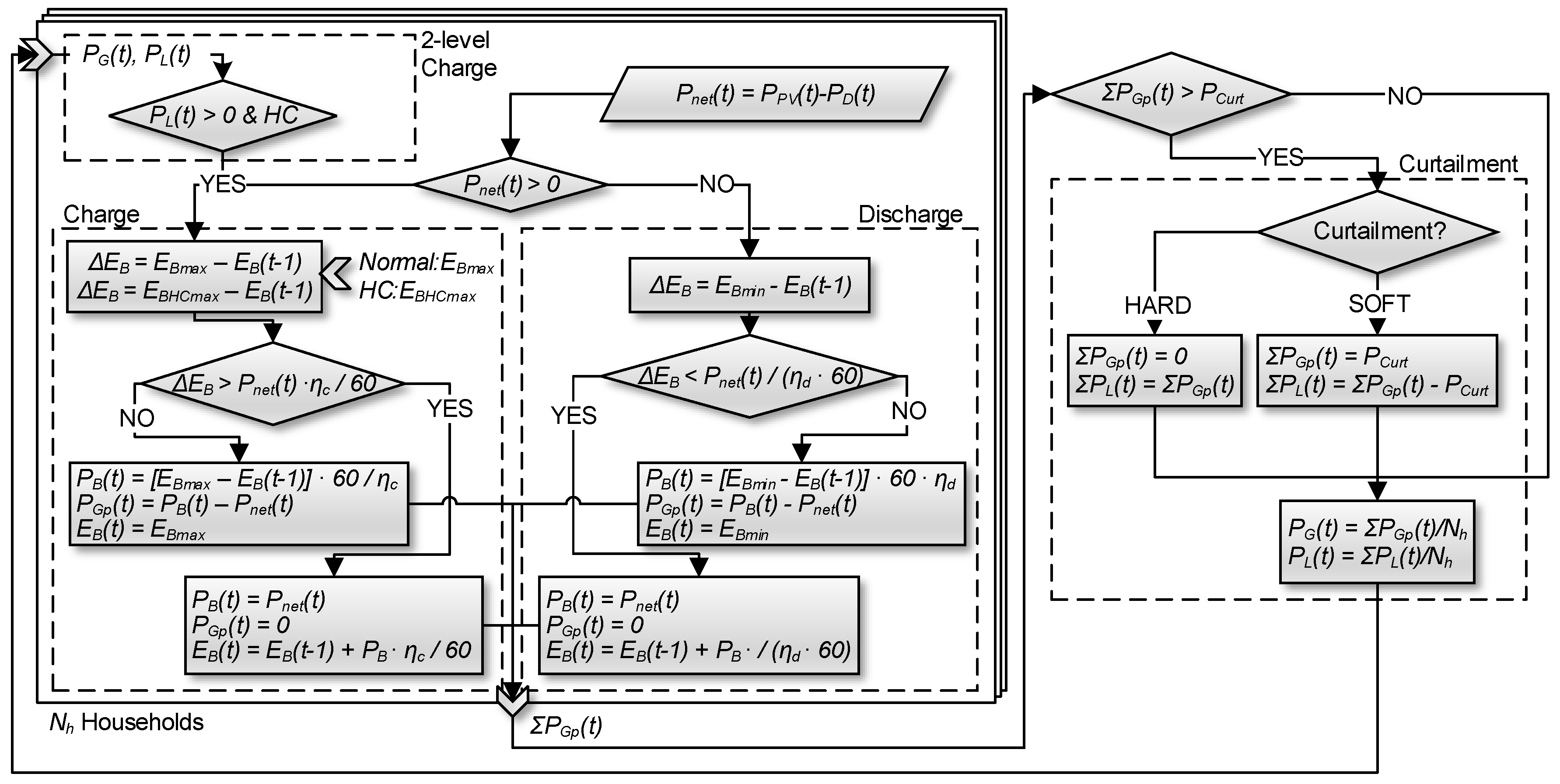
The interaction between the elements is indicated in Figure 3, where the flowchart of the process can be seen. As can be observed, the difference $P_{net}\left(t\right)$ between the production $P_{PV}\left(t\right)$ and the demand $P_D\left(t\right)$ is used to charge or discharge the battery between the energy limits $E_{Bmin}$ and $E_{Bmax}$. Subsequently, the deficit or excess of power that must be taken or injected into the grid $P_{Gp}\left(t\right)$ is calculated for each household.

Nevertheless, in case the sum of the power injected by the $N_h$ households exceeds the maximum power that can be injected into the grid $P_{Curl}$ for a given type of Curtailment, the above-mentioned strategies indicated in (5) for the soft curtailment and (6) for the hard curtailment are applied. The power that is lost and must be reduced in the PV production ($P_L$) due to the impossibility of being neither injected into the grid nor stored is also calculated for each curtailment.

Finally, the actual power applied to the battery system of each household $P_B\left(t\right)$ is lastly calculated sharing the grid capacity $P_G\left(t\right)$ and the power lost due to the curtailment $P_L\left(t\right)$ between all the households.

2.3.2. SCEMS: PV HC Enhancement

The improved algorithm that is proposed in this work to increase the amount of production that can be integrated into the smart community is based on a two-level charging scheme, which is of special interest for PV installations. The danger of incurring in a network overload when PV generation is injected into the grid increases in the central hours of the day due to the higher levels of irradiance; therefore, an algorithm that allows two thresholds of charge might improve the utilization of the PV generation.

The first charging threshold is ruled by the same conditions as the previously exposed mechanism, storing energy when the PV production exceeds the demand. Nevertheless, in this case, the battery is not fully charged during this period, but only until a set limit $E_{BHCmax}$. In this way, a selected percentage $\%SO{C}_{HC}$ is reserved. This percentage $\%SO{C}_{HC}$ is used when a potential overload situation is detected, so the injected power is reduced. For this aim, part of the PV production is employed to charge the batteries, whereas the maximum power allowed by the DSO is exported into the grid.

$$\%SO{C}_{HC}=E_{Bmax}-E_{BHCmax}$$

(7)

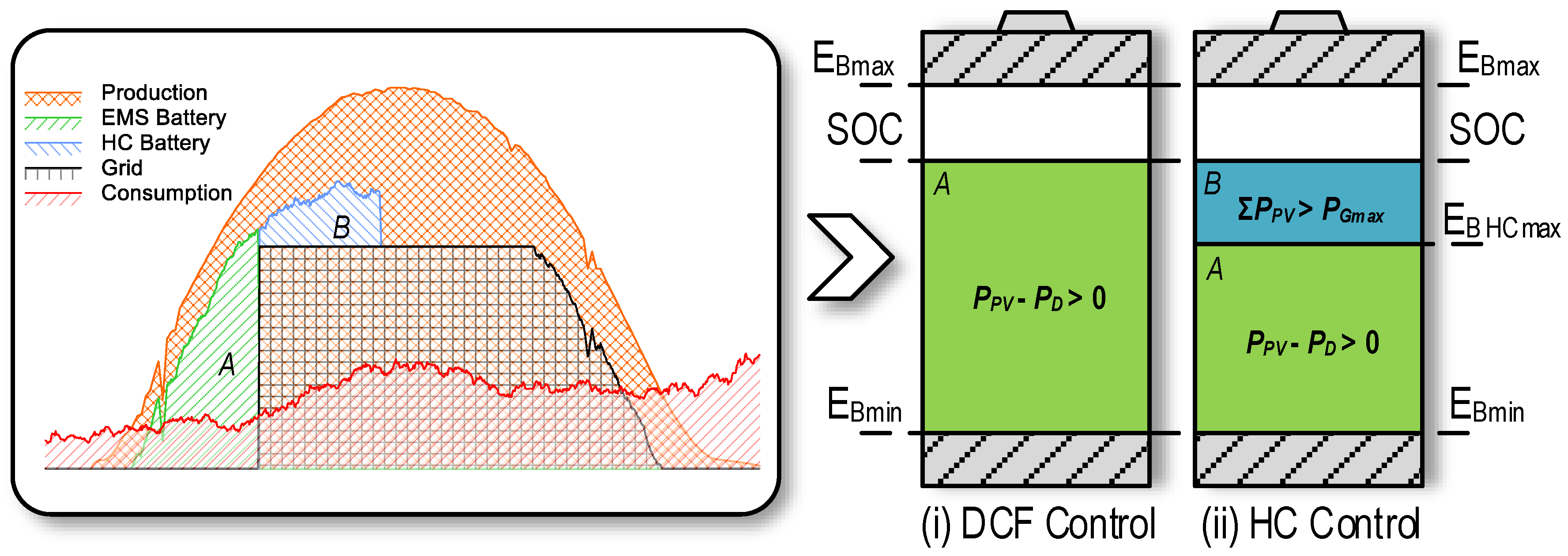
The proposed control strategy is illustrated in Figure 4 where the instantaneous daily profile together with the charging structure is shown. As can be seen, during the normal operation, the battery is charged as soon as the production exceeds the consumption, until the maximum allowed energy $E_{Bmax}$, as is depicted in (i), and the green area A is reached.

Using the new strategy proposed in (ii), the battery is divided into two levels. From $E_{Bmin}$ to $E_{BHCmax}$, the operation is the usual one illustrated by the green area A. However, a percentage $\%SO{C}_{HC}$ is reserved for the overload situation, as indicated by the blue area B. As can be observed in Figure 4 where the soft curtailment strategy is considered, under an overload situation, the power injected into the grid is set to the maximum allowed by the DSO, whereas the battery is charged for the blue area B.

The algorithmic behavior of the control system is almost similar to the one presented for the individual HEMS. Nevertheless, in this case, an additional charging operation is performed after calculating the production excess $P_L\left(t\right)$ as can be observed in the flowchart of Figure 3. What is more, the first charging limit in the normal operation is replaced by the new threshold $E_{BHCmax}$.

2.4. Evaluation Indexes

The performances of the system and the charging strategies were analyzed for different values of PV power and storage capacities with a set of indicators. Four indexes were selected to study the variations in the supply utilization, the percentage of self-consumption and the amount of energy that can be injected into the grid.

The first index was the demand cover factor (DCF), which aims to evaluate the percentage of self-consumption that can be achieved with the installed PV power. The second one was the supply cover factor (SCF) that indicates the percentage of utilization of the local generation. These two indexes are well defined in the literature, although different names can be found for them [25,26].

Their equations are indicated in (8) and (9) respectively, where $P_{PV}\left(t\right)$ is the instantaneous PV production, $P_B\left(t\right)$ is the instantaneous power supplied by ($P_B<0$) or applied to ($P_B>0$) the battery and $P_D\left(t\right)$ is the power demand. In addition, $t_0$ and $t_f$ define the temporal period for which the indexes are calculated. Therefore, different periods of time can be studied using the same expression and, in this case, the 1-min resolution power data in order to keep the temporal coincidence between production and demand.

$$DCF[t_0,t_f]=\frac{{\sum }_{t=t_0}^{t_f}min\left[P_{PV}\left(t\right)-P_B\left(t\right),P_D\left(t\right)\right]}{{\sum }_{t=t_0}^{t_f}{P}_D\left(t\right)}$$

(8)

$$SCF[t_0,t_f]=\frac{{\sum }_{t=t_0}^{t_f}min\left[P_{PV}\left(t\right)-P_B\left(t\right),P_D\left(t\right)\right]}{{\sum }_{t=t_0}^{t_f}\left(P_{PV}\left(t\right)-P_B\left(t\right)\right)}$$

(9)

However, those indexes do not take into account the interaction with the grid. Subsequently, a redefined SCF named as the ‘grid interaction supply cover factor’ (GISCF) is proposed by the authors. As is denoted in (10), this index includes a new parameter $P_G\left(t\right)$, which represents the instantaneous power exchange with the grid.

$$GISCF[t_0,t_f]=\frac{{\sum }_{t=t_0}^{t_f}min\left[P_{PV}\left(t\right)-P_{Batt}\left(t\right),P_D\left(t\right)+P_G\left(t\right)\right]}{{\sum }_{t=t_0}^{t_f}\left(P_{PV}\left(t\right)-P_{Batt}\left(t\right)\right)}$$

(10)

This parameter $P_G\left(t\right)$ is substituted by $P_{G_{soft}}\left(t\right)$ or $P_{G_{hard}}\left(t\right)$ when a curtailment is applied. Thus, the degree of utilization of the PV production can be studied not only under self-consumption conditions, but also when considering power injection into the electrical network.

$$EEF[t_0,t_f]=GISCF-SCF$$

(11)

Finally, another indicator is proposed in (11), extracted from the combination of the SCF and the GISCF. Named as the ‘exported energy factor’ (EEF), it accounts for the difference between the maximum amount of energy that can be injected into the grid and the percentage of production that is used for self-consumption. Therefore, this index indicates the net amount of PV production that can be sold, having economic connotations since the balance between PV size and maximum injected energy along the year can be obtained using this index.

3. Results

Once the methodology of the system has been described, the obtained results are shown and discussed. First, the high temporal resolution simulations provided by the model are addressed from both the individual and the aggregate point of view. After this, the variation of the daily indexes proposed for studying the interplay between production, consumption and the main grid is illustrated. Finally, three different scenarios are presented on a yearly basis to study how the above-mentioned indexes vary with the PV power, the storage capacity and the proposed control strategies.

The simulation process was implemented using the JAVA programming language. This language and its object-oriented philosophy allowed a flexible implementation with interoperability between operating systems and other features required in this development such as database and network connectivity, concurrency and functional programming. The system was developed as a JAVA enterprise application and was provided with a RESTful application programming interface (API) and a database to store the required information illustrated by the dashed line boxes in Figure 2.

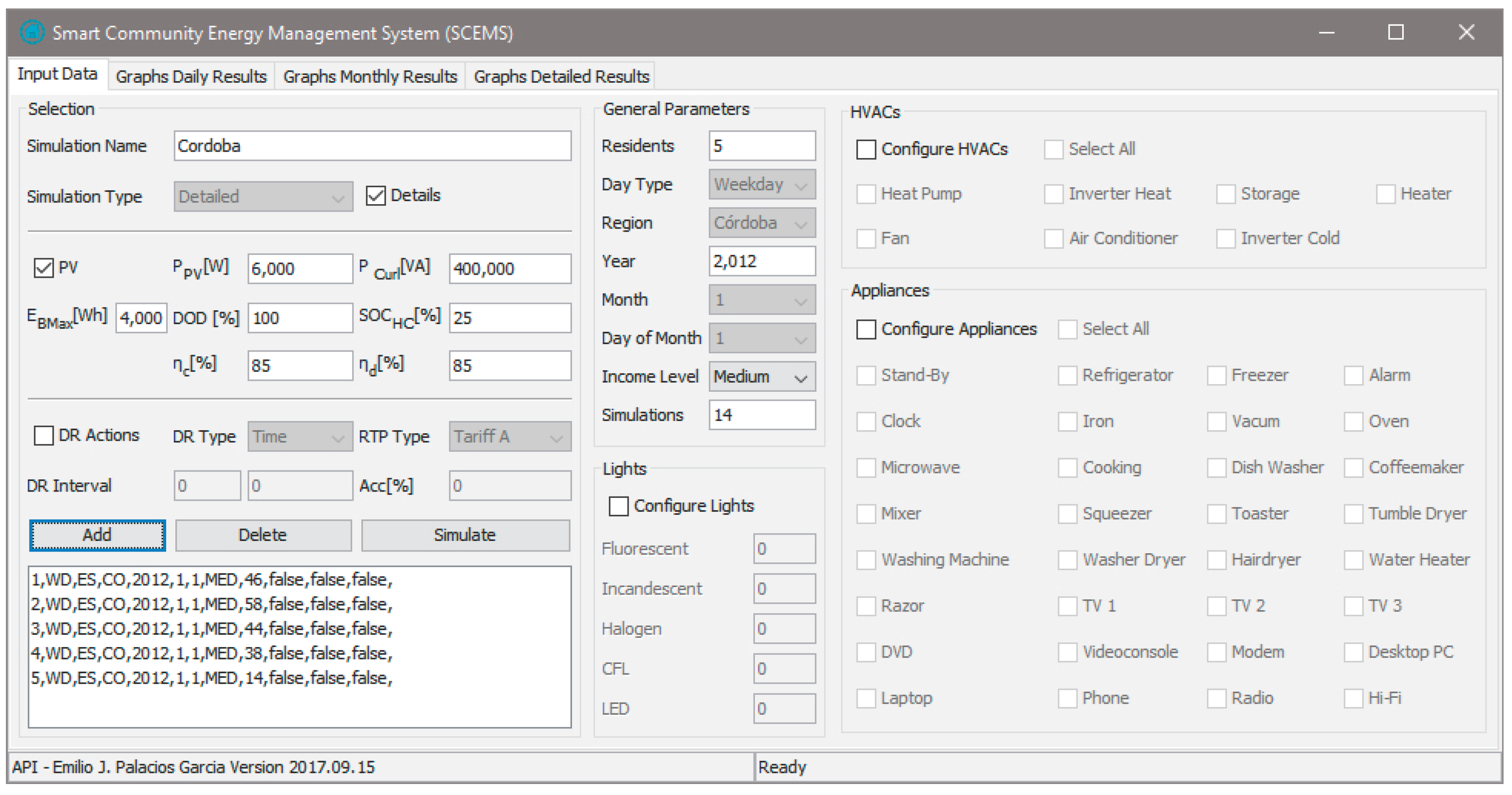
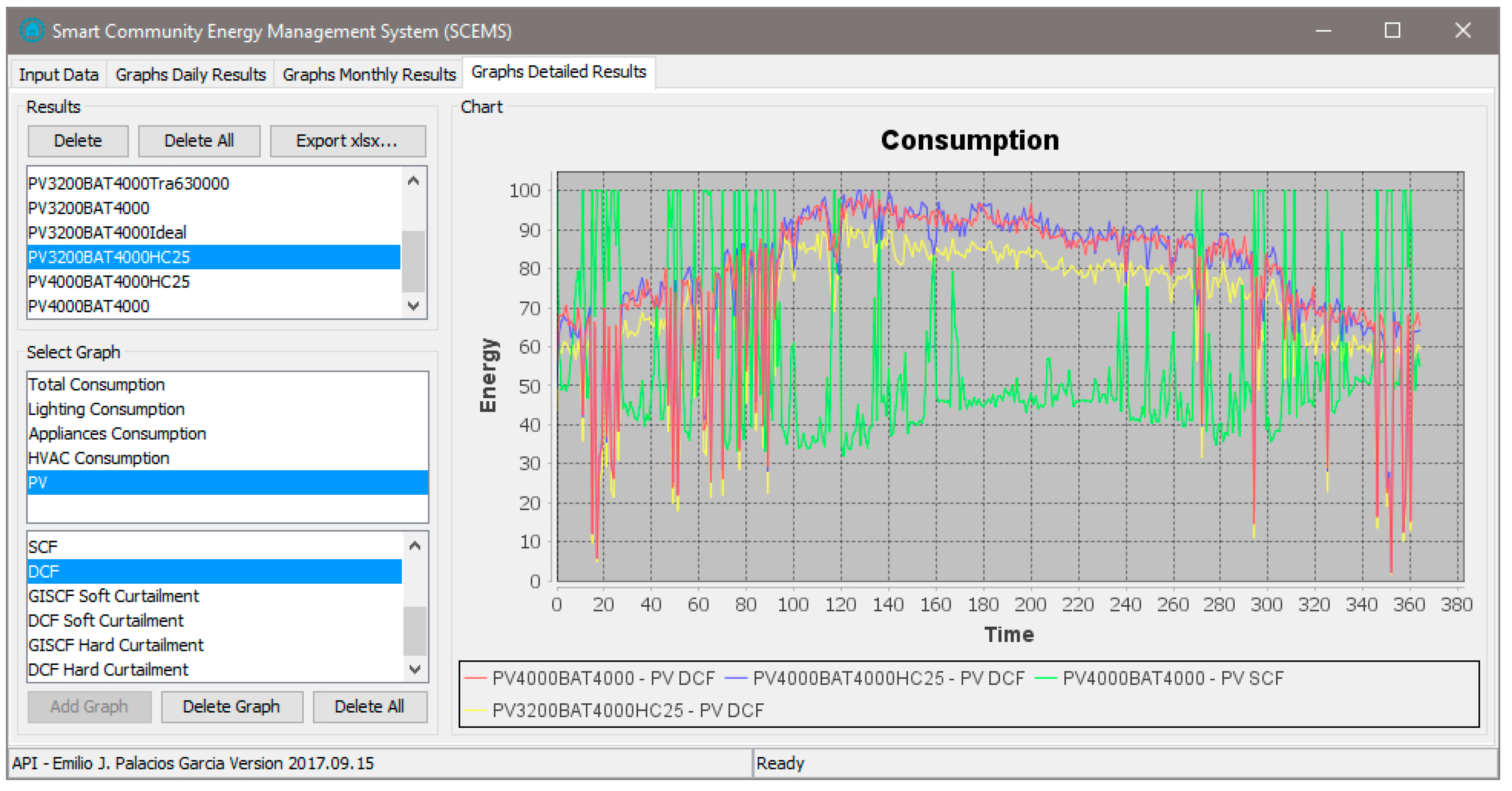
Using this API, the simulation parameters and the results can be sent to the system from any device that implements the HTTP protocol, increasing the usability and integrability of the system in other platforms such as MATLAB/SIMULINK for further network topologies’ processing. In addition, a general user application (GUI) was developed to ease the use of the system, where the simulation parameters can be configured using the configuration tab from Figure 5 and the results visualized as shown in Figure 6. This GUI is integrated into the previous one developed in [19].

3.1. High Temporal Resolution Simulations

The high temporal resolution of the model allowed analyzing the interplay between the consumer demand, the PV production, the energy storage system and the main grid with 1-min resolution. Moreover, as was indicated in the Methodology, the consumption model simulates each household individually so the daily profile of each dwelling can be observed, as well as the aggregate behavior.

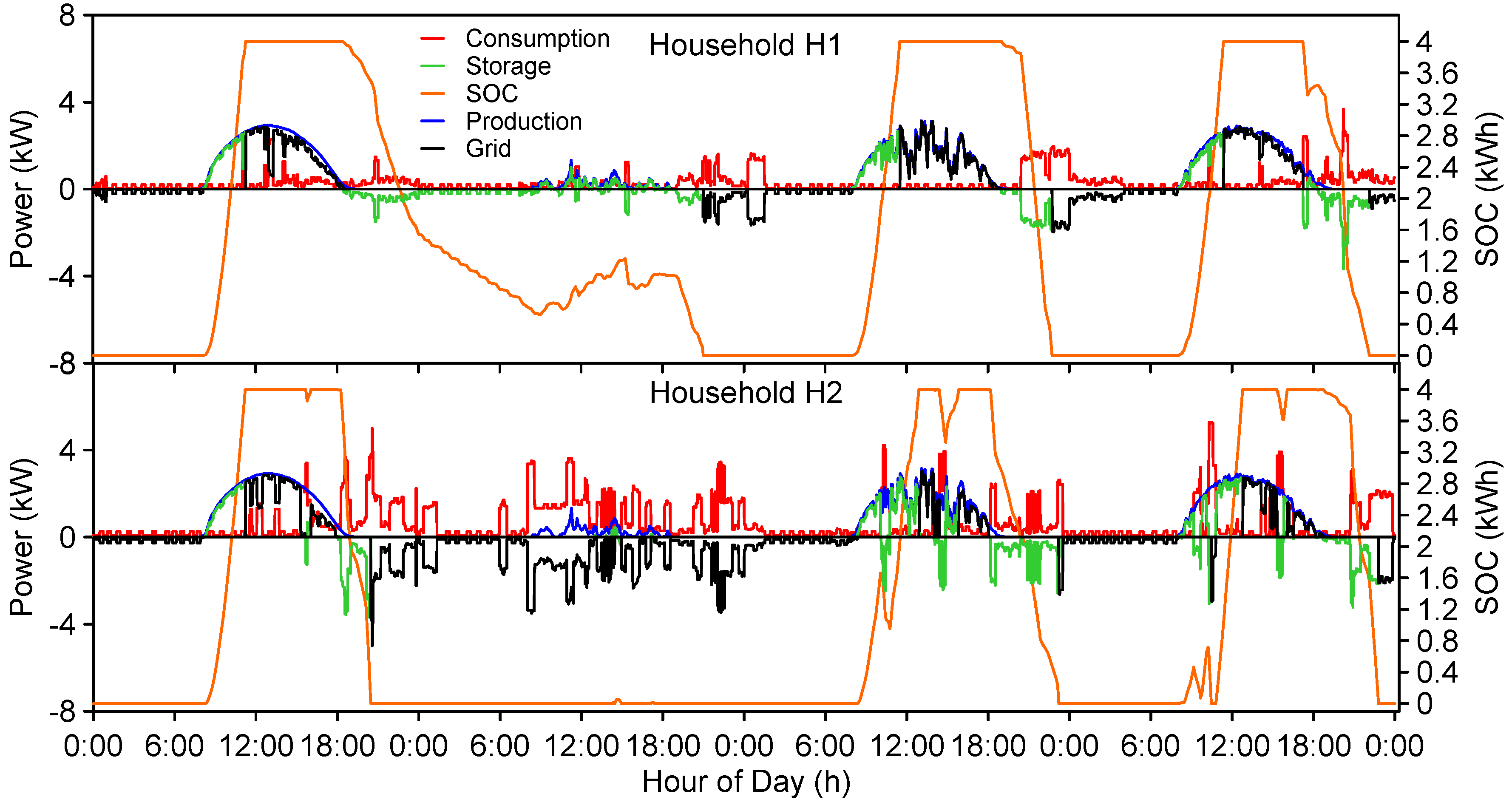
This fact is illustrated in Figure 7, where two individual households are represented from 18 to 21 March. Each household has the same 3200-W PV installation and 4000 Wh of energy storage, and they can interact with the main grid using the energy management strategy without HC enhancement.

As can be seen in Figure 7, the production profiles were similar since the two households are considered to be located in the same area. Nevertheless, the consumption profiles generated by the model were completely random, yet representing the aggregate trends observed in the region. This is one of the essential features and novelties of the model since each household has its individual and unique profile with a 1-min resolution, which even allows visualizing the on/off cycles of thermostat-controlled appliances such as refrigerators.

This has also a crucial impact on the calculation of the proposed indexes. In

Table 1. Indicator and energy figures for individual simulations. Comparison of 2 households. H, household.

Date	DCF (%)		SCF (%)		${\mathit{E}}_{\mathit{D}}$ (kWh)		${\mathit{E}}_{\mathit{PV}}$ (kWh)
	H1	H2	H1	H2	H1	H2	H1	H2
18 March	86.6	61.1	30.7	43.5	6.5	14.0	21.0	21.0
19 March	69.4	11.6	100	100	5.2	23.0	2.7	2.7
20 March	49.1	78.9	28.6	64.2	8.8	12.0	16.5	16.5
21 March	69.61	74.0	33.5	61.5	8.7	14.7	19.4	19.4

, the DCF and the SCF, as well as the daily energy demand $E_D$ and production $E_{PV}$ are indicated for the two households (H1 and H2) without taking into account the grid interaction. Some important conclusions can be drawn by observing both Table 1 and Figure 7.

For 18 March, the DCF of H1 was higher than the DCF of H2, whereas the SCF of H2 was higher. This means that the self-consumption rate of H1 was higher as might be expected due to the lower demand for the day. However, the direct utilization rate of the PV production was higher for H2, since demand and production were coincident in time, even though the demand was almost double for H2. The same trend was observed for 19 March.

For 20 and 21 March, in contrast to the previous results, the DCF of H2 was higher than the DCF of H1 even when the demand of H2 was almost double. In addition, the utilization rate (SCF) was higher for H2. That points out the importance of high-resolution simulations since, although the demand of H2 was higher, it temporally matched the production, and subsequently, both indexes were improved. This situation could not have been observed if merely the daily energy figures had been taken into account.

Additional conclusions can be obtained if a cluster of 200 households similar to the previously studied ones is simulated for the same range of dates (18–21 March). As can be seen in Figure 8, although the consumption profiles were stochastically obtained, the aggregate trend presented the expected behavior with two consumption peaks located during middays and evenings.

Regarding the aggregate PV production, when the whole system was taken into account, an overload occurs for 18, 20 and 21 March. In this case, a soft curtailment strategy was selected, and no HC enhancement was used, so a certain amount of energy $E_L$ is lost.

The figures of the cluster of households are presented in

Table 2. Indicator and energy figures for the aggregate simulation of 200 households.

Date	DCF (%)	GISCF (%)	${\mathit{E}}_{\mathit{D}}$ (MWh)	${\mathit{E}}_{\mathit{PV}}$ (MWh)	${\mathit{E}}_{\mathit{Buy}}$ (MWh)	${\mathit{E}}_{\mathit{Sell}}$ (MWh)	${\mathit{E}}_{\mathit{L}}$ (MWh)
18 March	85.0	92.7	1.936	4.191	0.329	2.222	0.100
19 March	27.8	100	1.896	0.541	1.370	0	0
20 March	83.0	98.8	1.957	3.298	0.333	1.396	0.017
21 March	84.6	98.3	1.920	3.890	0.297	1.971	0.034

using the GISCF since the interaction with the main grid is considered. The results show that for good days, the self-consumption factor DCF might achieve values in the range 80–85%. However, for very low production days, it might decrease down to 1/4, making it necessary to import a large amount of energy from the grid. Regarding the percentage of exported energy, even when the soft curtailment is considered, the percentage was higher than 90%.

3.2. Evaluation Indexes

The previous results showed the novel features of the model, but they only represent some specific days of a whole year. Therefore, the annual simulation of the proposed indexes was performed using different rates of installed PV peak and storage capacity per household, as well as different curtailment strategies. Again, a cluster of 200 households that represents the average users connected to an MV/LV transformer in the studied region was used, each of the households having the same PV power and storage capacity.

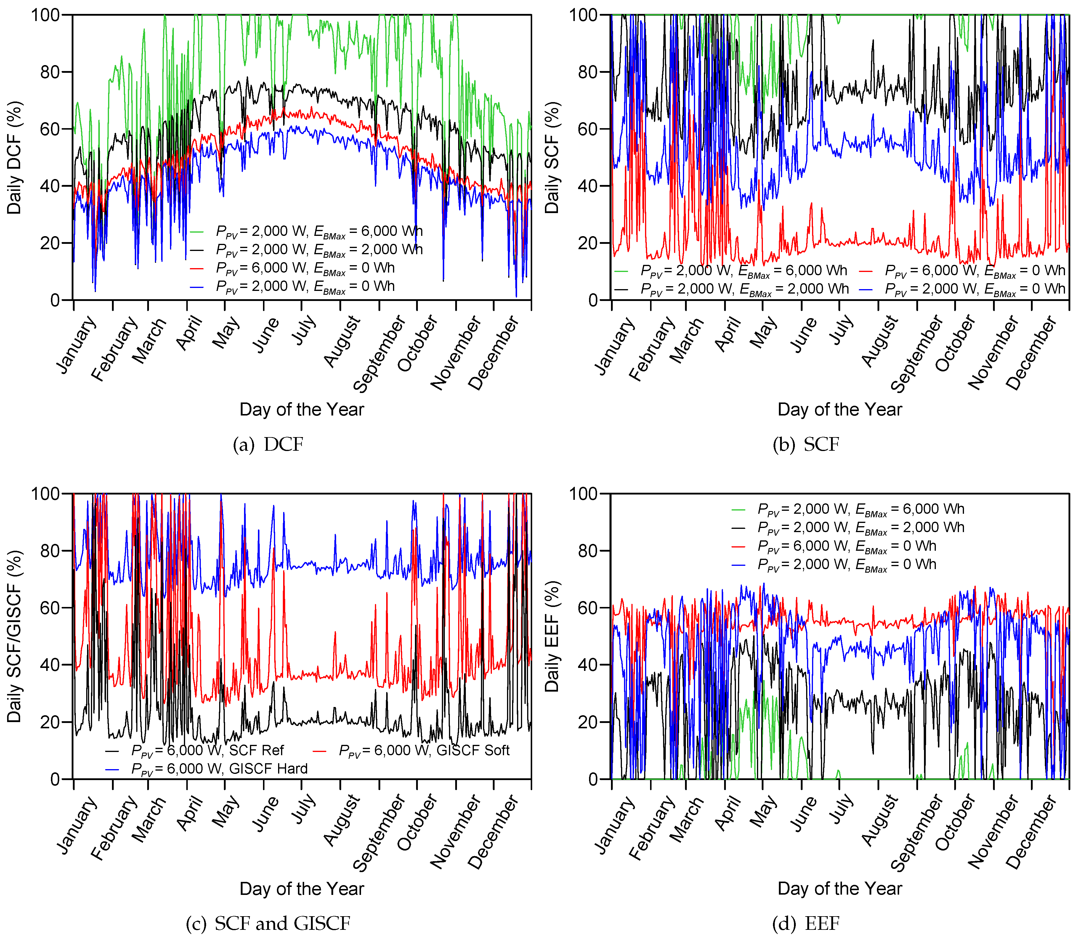
In Figure 9, the daily proposed indexes for a whole year are represented. In Figure 9a, the DCF is illustrated for different values of PV power and storage per household. As can be seen, an increase in the battery capacity produced a far more significant improvement in the DCF than a larger PV installation. Regarding the SCF in Figure 9b, large PV installations always worsened and decreased the degree of utilization, whereas, on the contrary, high values of battery storage improved the index.

Figure 9c presents the SCF when no interaction with the grid is allowed (black line). It depicts the low degree of utilization of the solar resource in islanded installations due to the non-temporal coincidence of production and consumption. When the excess of PV production was allowed to be injected in the grid according to some curtailment strategy, the increment in the utilized energy was 20% for the hard curtailment (red line) and 60% for the soft curtailment.

Finally, as regards the EEF in Figure 9d, it decreased when the battery capacity was increased, since more energy could be locally collected instead of being injected into the grid. However, when the PV power was increased such as in the case of the red solid line, the EEF mainly increased during the summer months with good production days, yet for some days, the values were lower since the energy injected had to be curtailed.

3.3. Yearly Calculated Index Scenarios and EMS Strategies

The previous calculations have shown some initial results about the influence of the PV power and the storage capacity in the proposed indexes. Nevertheless, another interesting feature of the model is that Expressions (8)–(11) can be extended to different periods of time such as a whole month or year by modifying the limits $t_0$ and $t_f$ for the instantaneous calculus. In this way, the annual average evolution of these figures was observed in three scenarios using the same cluster of 200 households and varying the installed PV power and storage capacity per household.

3.3.1. Off-Grid System

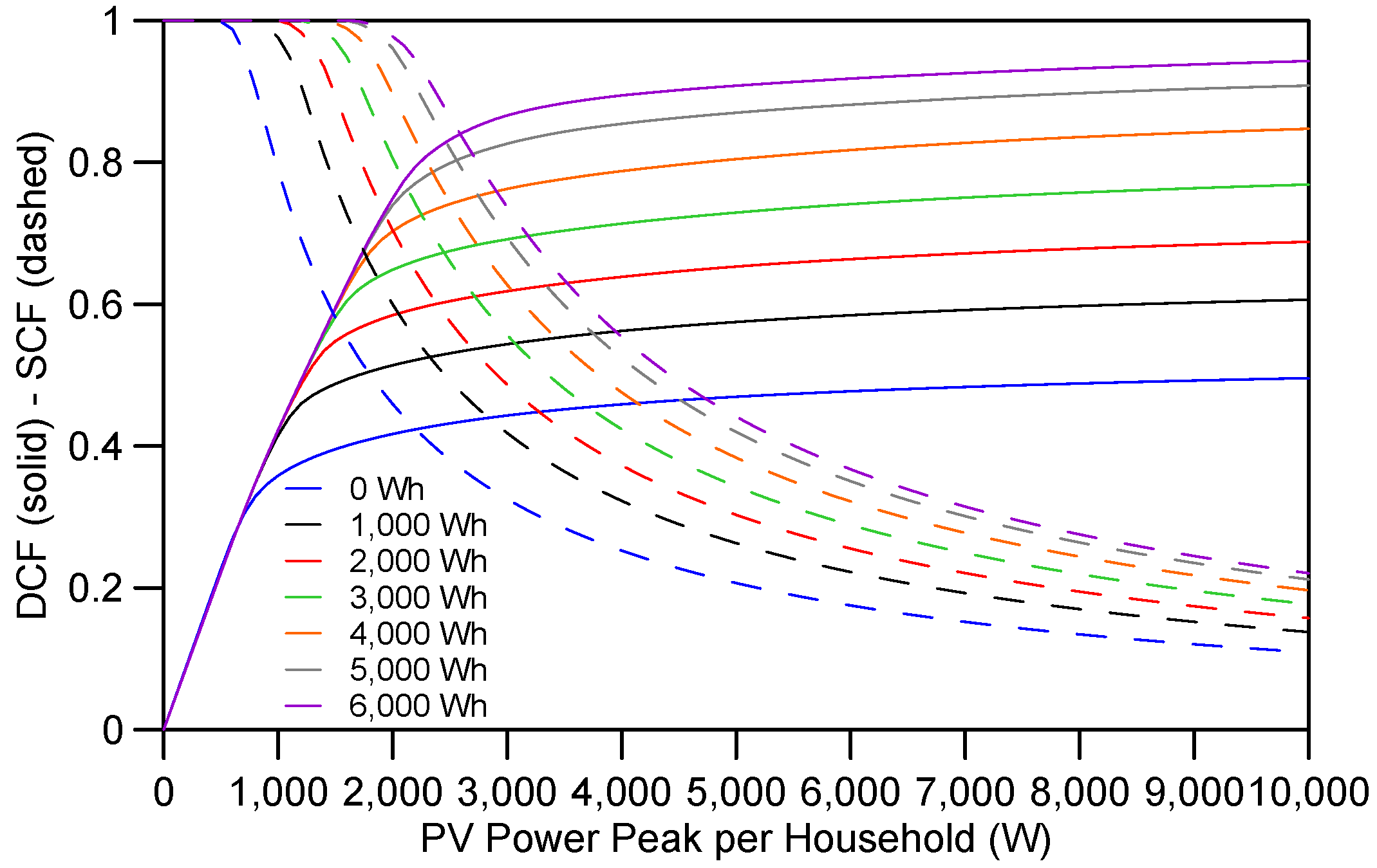
The base scenario without grid interaction was analyzed. The obtained results are shown in Figure 10, where the X-axis represents the installed PV power peak per household, whereas the Y-axis indicates either the annual DCF (solid lines) or the annual SCF (dashed lines). In addition, the different storage capacities per house are illustrated in different colors.

Figure 10 depicts how the DCF (solid lines) increased when the PV power peak increases, whereas in the case of the SCF (dashed lines), the opposite trend was observed. In contrast, for a given PV power peak, if the capacity of the storage system was increased, both the DCF and the SCF were improved, but not by the same percentage.

3.3.2. Grid Interaction

The base scenario exposed that in the case of off-grid systems, both a high amount of installed PV power and storage capacity were required in order to cover the energy demand along the year, whereas a great amount of produced energy was lost, as well. However, when considering the interaction with the grid, part of this excess might be injected always considering the HC limitations.

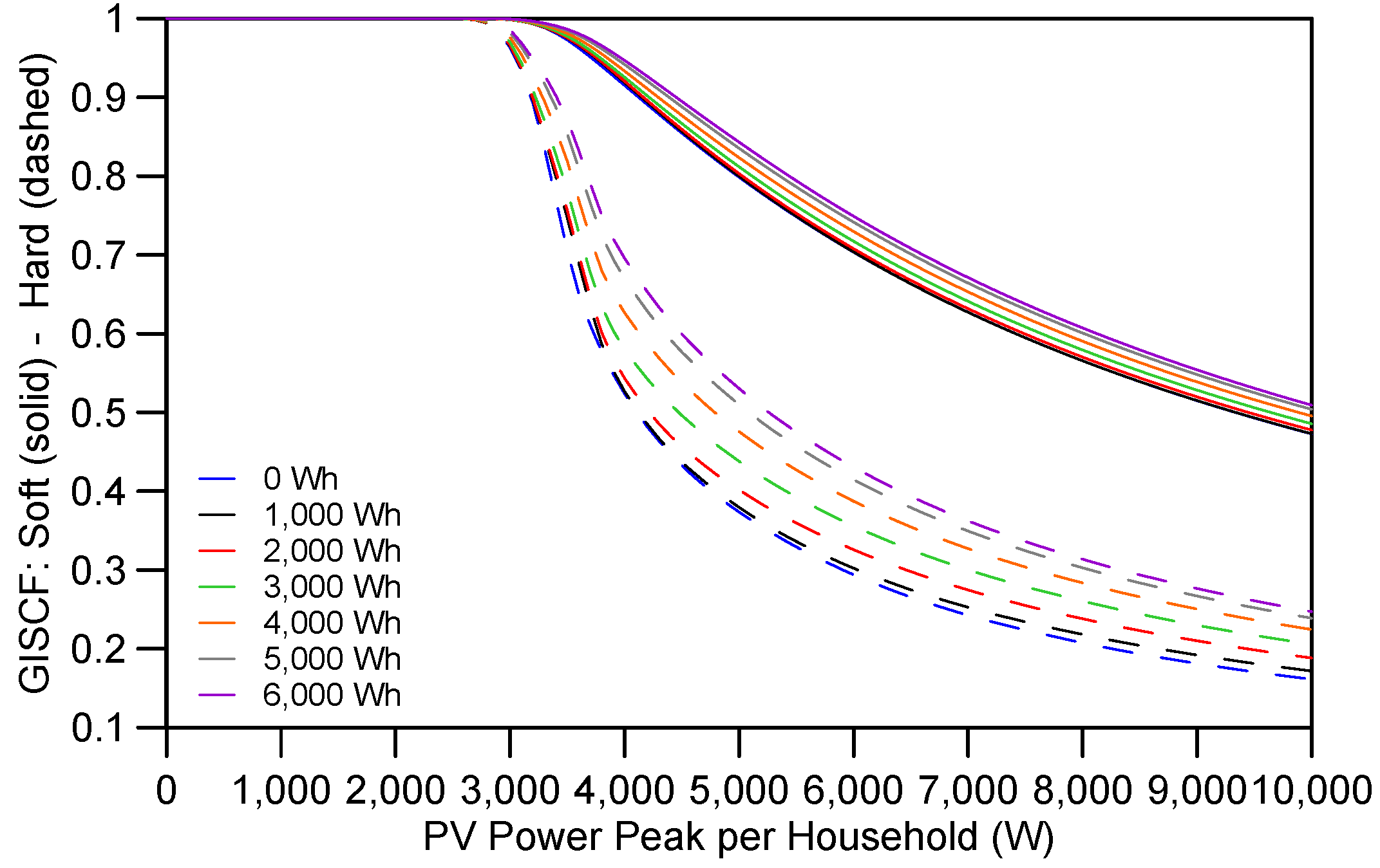
This interaction can be studied with the proposed GISCF as illustrated in Figure 11. The solid lines represent the soft curtailment strategy, whilst the hard curtailment situation is shown with dashed lines. As in the previous case, different storage capacity and PV power per household were studied considering an MV/LV transformer with a rated power of 400,000 VA.

As can be seen, the utilization degree was dramatically impacted by both HC strategies, but especially in the case of hard curtailment, where the energy lost due to the operative limits of the network was 40% higher. In addition, it can be pointed out that, although a higher storage capacity increased the degree of utilization, its impact was not very significant with an improvement of only 5% per 1000 kWh of installed capacity.

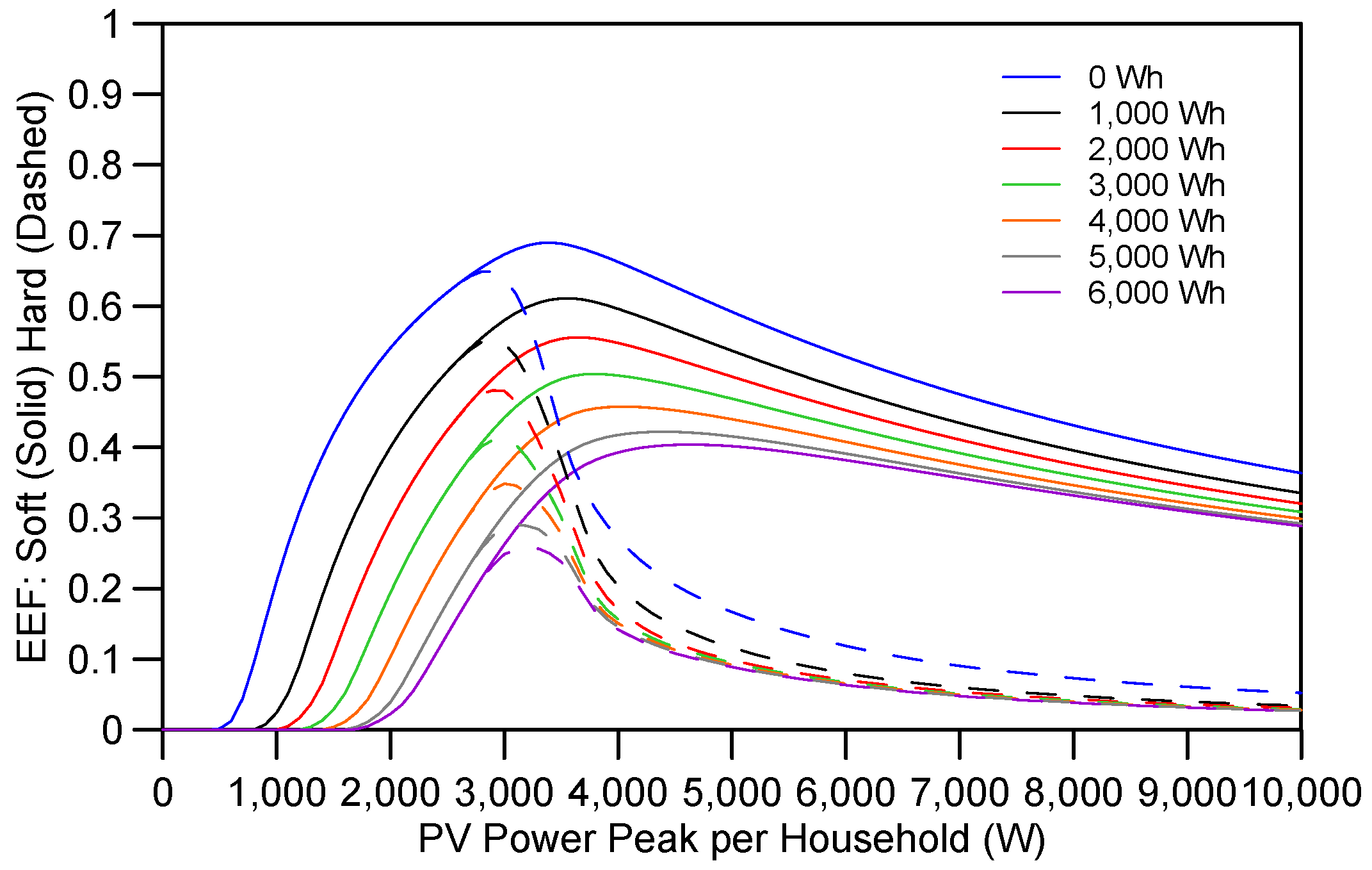
Further conclusions can be drawn if the EEF is studied. Figure 12 represents the proposed index to quantify the amount of injected PV production (EEF). Again, the soft curtailment situation is represented by the solid lines, whereas the dashed lines illustrate the hard curtailment strategy.

Figure 12 depicts that the injected generation was not directly proportional to the PV installed power, but under the curtailment situation, a given amount of PV power existed for which the energy exported to the grid was maximum, which was in fact slightly different for each curtailment situation. This result is especially relevant for planning PV installations, since the exported energy can be maximized and, subsequently, the benefits obtained from feed-in tariffs, whilst minimizing the initial investment and the payback period.

3.3.3. PV HC Enhancement

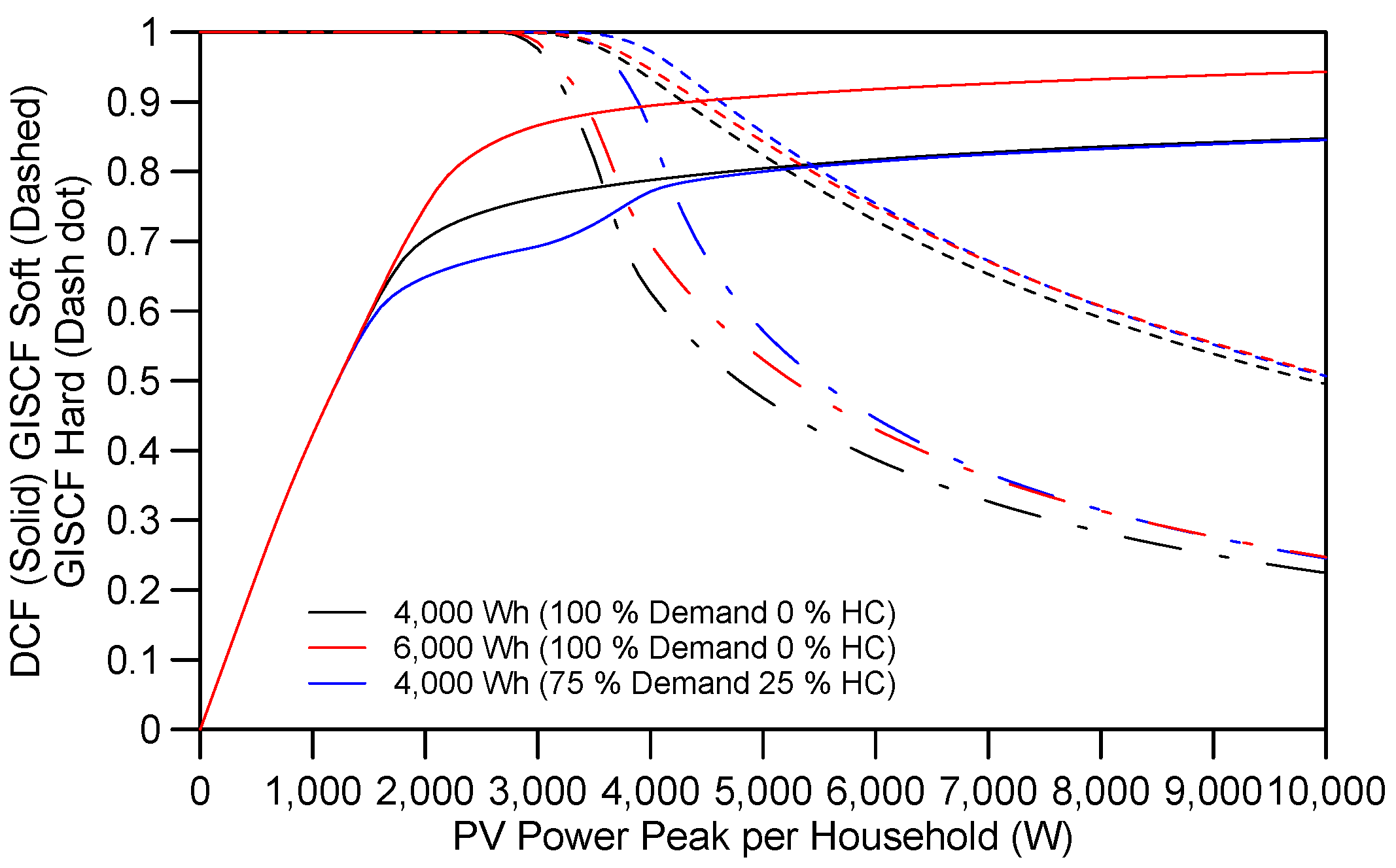
Finally, the third scenario illustrates the impact of control strategies focused on the enhancement of the HC. Since this control strategy depends on the battery capacity, three situations were considered, which are 4000 Wh of storage capacity per household and no enhanced control, 6000 Wh per household and no enhancement and 4000 Wh per household with two-level control using 75% of the capacity for individual control (HEMS) ($E_{HCmax}$), whereas keeping a 25% available for HC strategies of the whole smart community (SCEMS).

The results can be seen in Figure 13 where the three situations were represented. Black lines correspond to the 4000 Wh storage system with no enhancement; the red lines represent the 6000-Wh storage and no enhancement; and the blue lines are the proposed control algorithm to improve the HC. On the X-axis, different PV power peaks per household are illustrated, whereas the Y-axis accounts for the value of the indexes, which are the DCF (solid lines) and the GISCF both for the soft-curtailment situation (dashed lines) and the hard-curtailment strategy (dash-dot lines).

As can be seen in Figure 13, increasing the individual battery capacity improved the DCF by around 10%. However, the GISCF was almost unaltered showing an extremely small improvement. Nevertheless, when the HC enhanced algorithm was applied, the GISCF improved around 15% in the case of hard curtailment and around 5% for the soft curtailment when the values of PV power installed were not excessively large. If high installation rates of PV power are to be controlled with this strategy, a large percentage of battery should be devoted to the HC strategy or it should also be combined with an increase in the storage capacity.

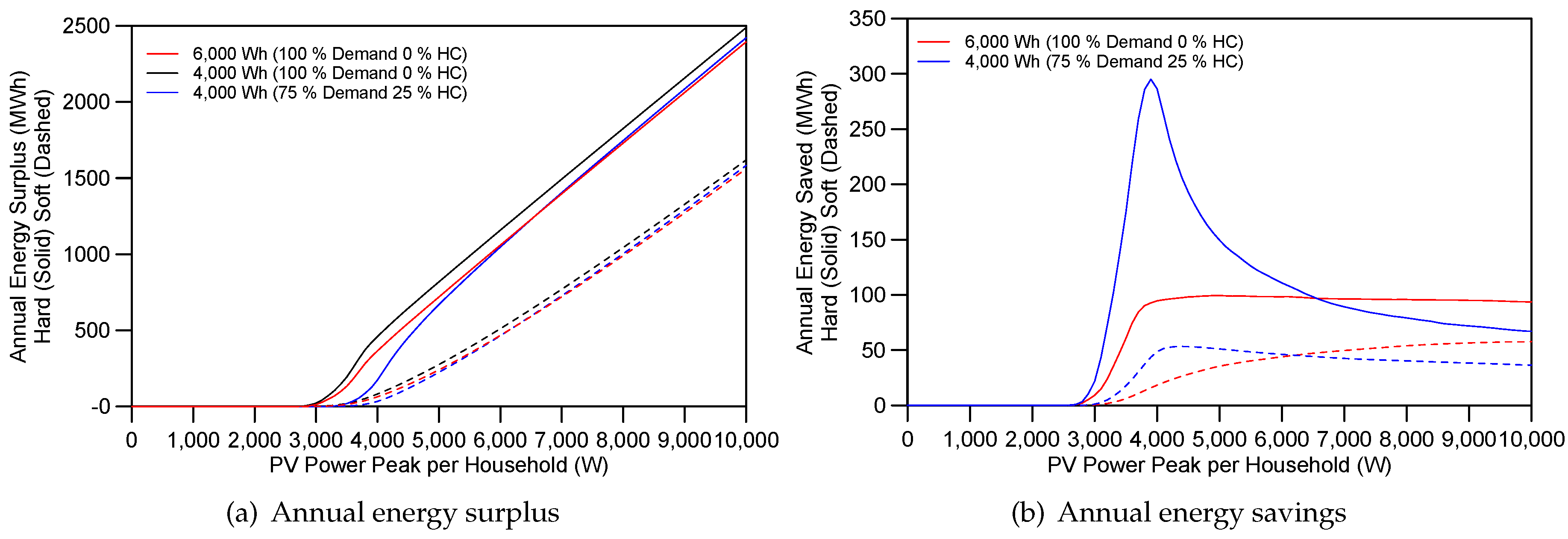
In addition, as is shown in Figure 14, the amount of energy that can be prevented from lost for a year in the whole cluster of households is very significant, especially in the case of hard curtailment situations. Using a larger local capacity saved around 50 MWh for the soft curtailment and 100 MWh for the hard curtailment. Opposed to this, with the new two-level charging strategy, the same savings were achieved for the soft curtailment with almost half of the PV power. In the case of the hard curtailment, a peak of 300 MWh was reached when 4000 W of PV power per household were considered, which means around 25% of the total annual consumption of the whole cluster of households.

It can also be noticed that the DCF was affected by PV power values that do not cause a serious energy surplus in the main grid (0–3000 W). Regarding this, two options can be adopted. On the one hand, a variable $E_{BHCmax}$ can be calculated so the fixed 75% value proposed in Figure 13 can be dynamically changed along the year depending on the irradiance forecasting. On the other hand, the enhanced algorithm can be chosen to be applied only for large PV powers.

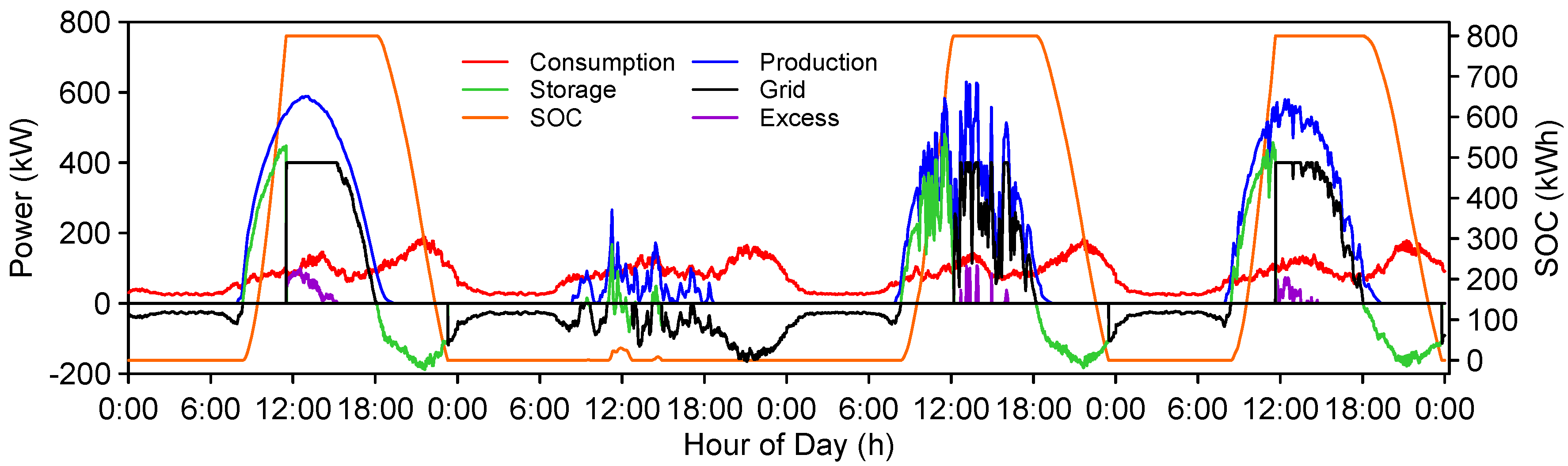
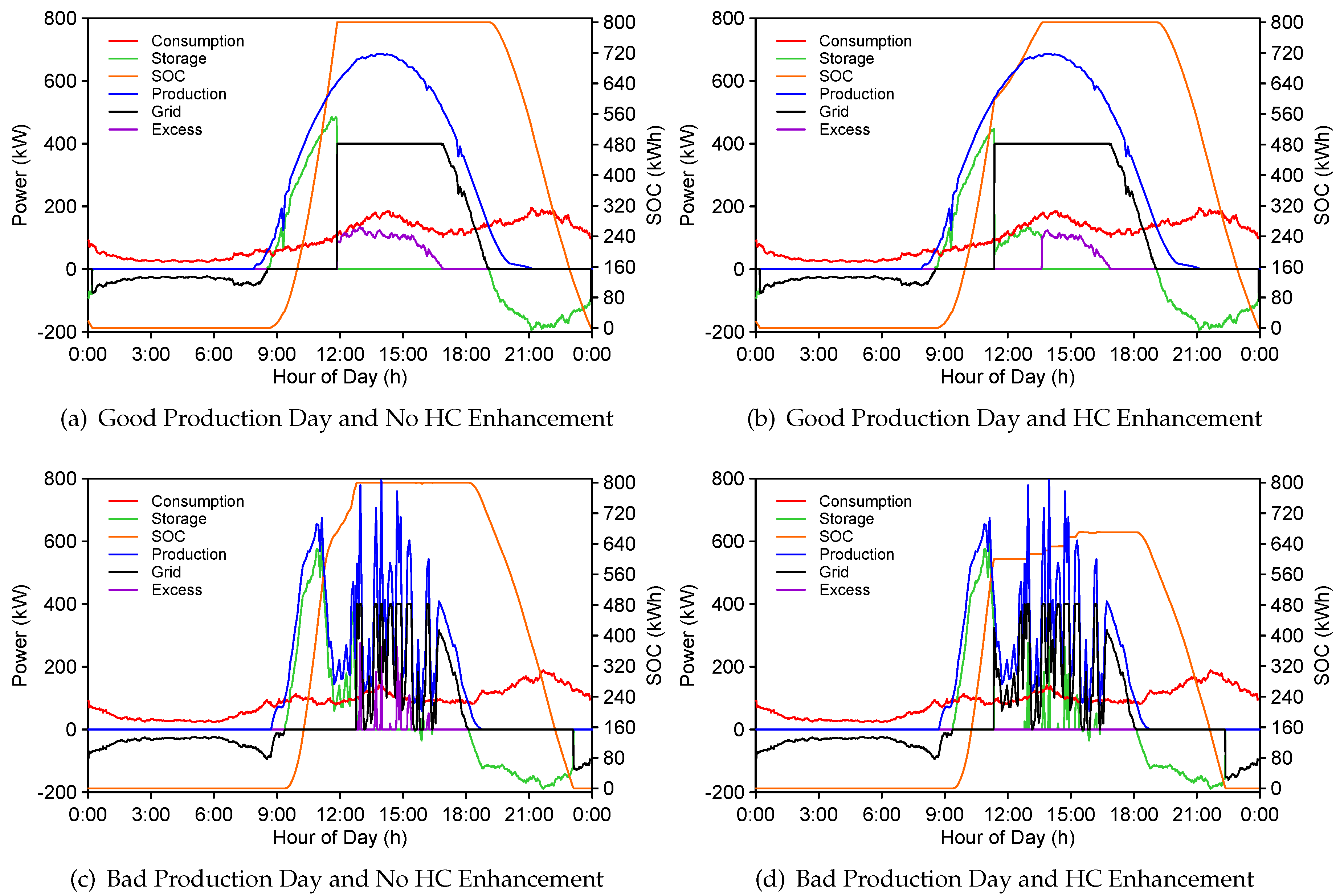
The reason for the DCF decrease can be seen in the high temporal resolution results represented in Figure 15 for a good production day (a) and (b) and a bad production day (c) and (d).

As can be seen when comparing Figure 15a,b, for a good production day, the two-level battery management algorithm allowed reducing the energy that is lost due to the soft curtailment, whilst the storage was fully charged. Thus, almost the same DCF cover factor was reached in both cases as can be seen in

Table 3. Indexes and energy for 2 days with and without HC enhancement strategy.

Type of Day	DCF (%)		GISCF (%)		${\mathit{E}}_{\mathit{Buy}}$ (kWh)		${\mathit{E}}_{\mathit{L}}$ (kWh)
	No HC	HC	No HC	HC	No HC	HC	No HC	HC
Good Production	87.5	87.4	90.6	94.6	292.2	292.8	470.5	271.3
Bad Production	77.0	71.6	96.8	100	477.3	587.5	86.7	0

, whereas the GISCF was increased in the enhanced case and the energy lost $E_L$ reduced to zero. However, in the bad production day, shown in Figure 15c,d, the selected $E_{BHCmax}$ prevented the storage system from being fully charged during the day for the enhanced strategy (d), and therefore, the DCF was lower. Nevertheless, the amount of lost energy was null as indicated by the GISCF of 100%.

If both the energy imports from the grid $E_{Buy}$ and the energy lost due to the soft curtailment $E_L$, indicated in Table 3, are taken into account, it can be observed that the balance is positive or zero. In the case of a good production day, when the enhanced strategy was applied, the energy saved was 199 kWh, while the energy that needed to be imported from the grid was the same for both controls. Likewise, in the bad production day, although 110 kWh extra had to be imported from the grid in the enhanced strategy, 87 kWh were prevented from being lost, compensating the decrease in the DCF.

Therefore, although the proposed two-level charging control might have an impact on the DCF, if the whole cluster of households and its interaction with the main grid are considered, the stability of the network will not only be guaranteed, but the utilization rate of the PV installation will also increase.

4. Conclusions

A high temporal resolution simulation environment has been presented that allows assessing the integration of distributed renewable energies and storage systems in households, whilst interacting with the main grid, by means of a stochastic demand model and historical data from a PV installation.

Various evaluation indexes have also been proposed in this work. Along with the previously defined DCF and SCF, the authors have developed and used two new indicators named GISCF and EEF. The first index allows assessing the renewable production utilization when the system interacts with the main grid under some constraints such as the HC of the network. This index has been shown to be valid to quantify the impact of curtailment strategies when both the PV production and the capacity of the battery storage system are incremented.

The second index, EEF, has proven its application in the context of energy planning for assessing the most suitable combination of PV power and storage capacity that might allow maximizing the power injected into the grid. Therefore, in a context where feed-in tariffs are applied, it would help choose the initial investment and minimize the payback period.

Using the models and the evaluation indexes, a series of high-temporal simulations have been performed, showing the possibilities of the system from the individual and the aggregate point of view. Likewise, the yearly evolution of the proposed indicators has been studied for different rates of PV power and storage capacity per household.

Based on the previous results, three scenarios were evaluated for a whole year and for different rates of PV power and storage. The off-grid scenario showed the influence of the PV power and the battery capacity in the SCF and the DCF. Larger capacities always improved the both indexes, but the installation of more PV power only helps increase the DCF, whereas the SCF is worsened. The same results were obtained in the grid connected scenario, the newly developed indexes GISCF and EEF comprising a key point to assess the soft and hard curtailment strategies when interacting with the grid.

Finally, a novel two-level charging strategy has been proposed aiming to maximize the renewable energy utilization, while preventing the network overload. The algorithm has shown a substantial improvement of the GISCF, and although the DCF is worsened in some cases, the amount of energy that is prevented from being lost fully justified its use.

This DCF decrease can be corrected with the use of a dynamic $E_{BHCmax}$, taking into account the energy demand prediction, as well as the production forecast and the capacity of the transformer itself. In this way, not only the GISCF will be improved, but the DCF will also remain almost unaltered. Therefore, future works will be focused on the development of a predictor for the $E_{BHCmax}$ based on the irradiance and the demand estimation.