Comparative Study on Uni- and Bi-Directional Fluid Structure Coupling of Wind Turbine Blades


1
School of Mechanical and Electrical Engineering, Wuhan University of Technology, Wuhan 430070, China
2
Department of Mechanical Engineering, Woldia University, Woldia, Ethiopia
*
Author to whom correspondence should be addressed.
Energies 2017, 10(10), 1499; https://doi.org/10.3390/en10101499
Submission received: 26 July 2017
/
Revised: 31 August 2017
/
Accepted: 1 September 2017
/
Published: 27 September 2017
Abstract
:The current trends of wind turbine blade designs are geared towards a longer and slender blade with high flexibility, exhibiting complex aeroelastic loadings and instability issues, including flutter; in this regard, fluid-structure interaction (FSI) plays a significant role. The present article will conduct a comparative study between uni-directional and bi-directional fluid-structural coupling models for a horizontal axis wind turbine. A full-scale, geometric copy of the NREL 5MW blade with simplified material distribution is considered for simulation. Analytical formulations of the governing relations with appropriate approximation are highlighted, including turbulence model, i.e., Shear Stress Transport (SST) k-ω. These analytical relations are implemented using Multiphysics package ANSYS employing Fluent module (Computational Fluid Dynamics (CFD)-based solver) for the fluid domain and Transient Structural module (Finite Element Analysis-based solver) for the structural domain. ANSYS system coupling module also is configured to model the two fluid-structure coupling methods. The rated operational condition of the blade for a full cycle rotation is considered as a comparison domain. In the bi-directional coupling model, the structural deformation alters the angle of attack from the designed values, and by extension the flow pattern along the blade span; furthermore, the tip deflection keeps fluctuating whilst it tends to stabilize in the uni-directional coupling model.
1. Introduction
The wind turbine is one of the fast growing renewable energy sources across the globe for generating a capacity of 282.5 GW in 2013 and is expected to raise up to 1.1 TW by the end of 2020 [1]. The growing demand for wind energy drives the design trends toward larger blades; up to 125 m is achieved [2] with efficient aerodynamic and structural performance. The current wind turbines tend to be slender, lighter, more flexible, made of composite materials, and equipped with more complex control schemes [3]. However, such design trends are inherent with severe vibration loads and instability issues due to low stiffness and large deformation, which will reduce operational life and power production of the turbine. Along the individual effect of aerodynamic and structural performance, their coupling has a significant influence on the performance of wind turbines. Therefore, fluid-structure interaction (FSI) plays a significant role while dealing with such design trends, and thorough understanding of this interaction is required for efficient and reliable output.
The numerical approaches to simulate FSI problems can be broadly classified into two classes: the monolithic approach and the partitioned approach. The monolithic approach treats the fluid and structure dynamics in the same mathematical framework to form a single system of equation for the entire problem, while the partitioned approach considers them as two computational fields to be solved separately [4]. As of the partitioned approach, wind turbine FSI can be treated with a different fidelity level, as in classical aeroelastic methods where the fluid and structure interaction are treated separately and uncoupled [5], to recent full coupling to capture the real time interaction [6]. Most low fidelity methods incorporate classical models such as the blade element momentum theory and low order structural models, with loss or one-way fluid structure interaction, which are fast and cheaper to implement. However, they are inadequate for handling complex geometries and material variations, unsteady and turbulent flows, and their approximations are inaccurate for such applications. Conversely, recent aeroelastic simulation tools are capable of simulating a full-scale 3D model of a wind turbine with fully turbulent flow condition to provide credible results, demanding highly accurate methods and strong fluid structure interaction approximations with numerical efficiency and stability. During recent decades, several numerical methods have been developed to simulate the full FSI, such as Arbitrary Lagrangian-Eulerian (ALE) methods [7,8,9] and the deforming-spatial domain/stabilized space-time (DSD/SST) methods [10,11], and other high order computational tools. Selecting an aeroelastic tool for a specific application falls under a compromise between the computational effort available and expected efficiency; therefore, an extensive investigation is required among these tools to understand their shortcomings and strengths for the intended application.
FSI of a wind turbine can be approximated with uni-directional (two-way) coupling or bi-directional (one-way) coupling. One-way FSI coupling requires reduced computational effort and fast execution; however, tightly coupled two-way coupling will provide more vivid and reliable results of the aeroelastic phenomena. Few comparison studies between the two coupling methods are done, such as Benra et al. [12], comparing them for different cases; for simple cases, the two methods have better agreement, whereas for complex cases the gap is significant and the one-way FSI model fails to work well. Therefore, two-way coupling provides more credible results. Chen et al. [13] also compared the two methods for micro (0.85 m rotor diameter) horizontal axis wind turbines; mechanical loading, torque, and power output were considered; typically, the equivalent stress was recorded to be maximum of 18.9 MPa and 21.3 MPa for the uni-directional and bi-directional method, respectively, and showed a unique distribution for each method. Kumar and Wuma [14] studied FSI for composite propeller blades and compared results based on uni-directional and bi-directional models, such as deformation, which is reported to be larger for uni-directional coupling because of missing cross coupling of solvers to take into account the flow change due to blade deformation. Few more researchers are also devoted to investigating the merits and limitations of the two coupling methods; however, computational demand restricted most of the researchers to deal with scaled wind turbines and few operational conditions, creating an enormous gap in the subject.
To enhance the performance and satisfy the complex design constraints of the wind turbine system, a comprehensive understanding of the aeroelastic characteristic of the system and an integrated optimization is vital. The present paper will take part by investigating a comparative study between uni-directional and bi-directional fluid-structure interaction models, considering a geometric copy of the NREL 5MW wind turbine blade [15]. To highlight the background of the problem, the mathematical formulations for fluid domain and structural domain, and also the fluid-structure coupling, are included. ANSYS Fluent and Transient Structural modules are employed for the fluid and structural domain, respectively, and the system coupling module is configured according to the coupling model selected.
2. Mathematical Formulation
2.1. Flow Model
Several flow models are available for wind turbine aerodynamics, such as Blade Element Momentum (BEM), actuator disk model, vortex model and others. However, one will apply Computational Fluid Dynamics (CFD) based tools which intend to incorporate Reynolds Averaged Navier-Stokes (RANS) equations to model the flows, with simplified closures. Navier-Stokes equations are comprised of the continuity equation and conservation of momentum equations along each coordinate. As of wind turbine application, the flow pattern is categorized as low Mach flow, nearly 0.1 [16]; thus, the incompressible flow model suits well. Therefore, N-S equations for three-dimensional incompressible flow will be:
where: : velocity vector, : air density, : pressure, : kinematic viscosity, and body force vector.
To alleviate the numerical difficulty to solve incompressible N-S equations, two common remedies are available: preconditioning and artificial compressibility. Applying the latter method, the artificial compressibility term will be added to the continuity equation and results (Equation (3)), pressure based or pressure corrected continuity equation.
where: is a pseudo speed of sound.
Finally, Equations (2) and (3) will be solved to determine the flow characteristic. One has chosen the pressure based solver scheme with coupled algorithm in which momentum (Equation (2)) and pressure based continuity (Equation (3)) are solved simultaneously. Pressure based coupled solver provides a merit of faster solution convergence rate as compared to the segregated algorithm, aside from its high memory requirement. Other parameters can be determined using energy equation and the equation of state relations, Equation (4).
Conservation of energy:
where: , : internal energy of the fluid, : is the rate of heat source, k: thermal conductivity, and also the relation between : temperature, : density and the equation of state, .
Closure for turbulence:
Flow around the wind turbine can be fairly considered as turbulent and so including the effect of turbulence in the flow model is mandatory. Several turbulence models are available, such as the Spalart-Allmaras model, two equations k-ϵ model and k-ω model, Reynolds stress model, Detached Eddy Simulation (DES), Large Eddy Simulation (LES) model, and others. Among those, Shear Stress Transport (SST) k-ω model will be utilized in this specific work. The SST k-ω model is a special treatment of the standard k-ϵ model in the far field and the standard k-ω near the walls [17,18]. The transport equation for k and ω will be expressed as [18]:
The generation terms of k and ω are and , respectively, with , and are the source terms for and , respectively, , and the term is the Reynolds stress tensor [12]; the dissipation terms are, and ; and the cross diffusion term that blends the two models is given by are the turbulent Prandtl’s numbers; are dynamic and turbulent viscosity; and the coefficients , , , and are damping functions, and can be determined based on Menter et al. [17,19].
The transport equations will be solved and modify the previous governing equations to include the effect of turbulence in the flow.
2.2. Structural Model
The structural dynamics of the blade can be described with a set of differential equations of motions and discretized and solved using the finite element analysis approach. In the earlier attempts to formulate the equation of the motion of a blade, the works of [20,21] developed an equation of motion for combined flapwise and chordwise bending and torsion of a twisted non-uniform rotor blade. More comprehensive models are developed subsequently to include pitch action, rotor speed variation, the effect of gravity [22], the coupling between blade and tower, and other phenomena.
For the present work, the formulation presented in [22] is adopted with constant rotor speed. Consider the following coordinates: In Figure 1, the Cartesian coordinate X, Y, Z is the inertial reference frame R, with Z-axis pointing downwind direction and the origin set at the center of the hub. The frame is rotating with the blade at a constant speed of Ω about Z-axis, with axis lies along the elastic axis (ea) of the undeformed beam, and is blade pitch axis. Note that frame is inclined with a pre-cone angle of βpc from the plane of rotation (Z, X). The two XΩ and YΩ axes are included in Figure 1 for the sake of clarity; they are found when the pre-coned axes rotate Ωt about the Z-axis. β is the pitch angle. The coordinate frame (x, y, z) is aligned with but rotating about the pitch axis , (see Figure 1); the transformation of these coordinates for the sake of brevity it is not discussed here, although thorough information is available in [22].
The generalized coordinate to express the location of a point on the blade, with u, v, w and are translational displacement of the point along, x, y, z and angular displacement about the x (pitch axis), respectively; , , , and (it included all angular displacement including elastic twist, control pitching, as well as the section built-in twist), written as Equation (7);
Dividing the blade into a finite number of segments or elements along the blade span (Figure 1), the equation of motion of the ith element of the blade can be formulated using the Lagrangian equation as follows:
where: Subsequently, the individual components of the above equation will be formulated for the ith element.
Considering uniaxial stress assumption, the elastic (strain) energy of the ith element can be defined as:
where: the stresses, , , , and the strains, , and , [20], : Young’s modulus (along the longitudinal direction) , : Shear modulus .
The gravitational potential energy of the ith element is given by:
where: is position vector for the center of gravity of ith element, : gravitational field, : mass of the ith blade element/segment, the product of density and elemental volume .
The kinetic energy of the ith element is also described as:
where: = the absolute velocity of the center of gravity of the ith element, : constant spinning speed of the rotor.
The generalized forces (such as aerodynamic forces), acting at the elastic axis of the section can be expressed as:
where: , and are the aerodynamic forces along u, v and w, respectively, and pitching moment about the pitch axis .
Substituting Equations (9)–(12) into Equation (8) will provide the equation of motion for the ith element as:
This equation of motion of each element will be assembled to give the system equation of motion of the whole blade as,
where: : the mass matrix, : damping matrix, and : stiffness matrix, the subscripts referring the ith element and for the whole blade assembly, respectively.
Finally, Equation (14) will be simultaneously solved to calculate displacements, velocity, and accelerations of each element. Based on these results, other structural parameters, such as reaction forces, moments, and stress, will be determined.
2.3. Coupling Methods and Algorithms
Considering the partitioned approach, once separate solutions are attained for each physical field (i.e., fluid flow and structural dynamics), the fluid-structure interface will serve as a boundary to communicate information among the two solvers.
The two separate fields are governed by the equations derived in the preceding sections.
For the structural domain:
For the fluid domain:
However, at the intersection of the two domains, the governing equations from both sides have to agree, imposing boundary conditions, i.e., no-slip, no-penetration, and traction conditions, mathematically expressed as Equation (15):
These boundary conditions will couple the two solvers and demand us to communicate them according to the available and required coupling strength on hand. For the present study, two fluid-structure couplings are considered: uni-directional (one-way) and strong bi-directional (two-way).
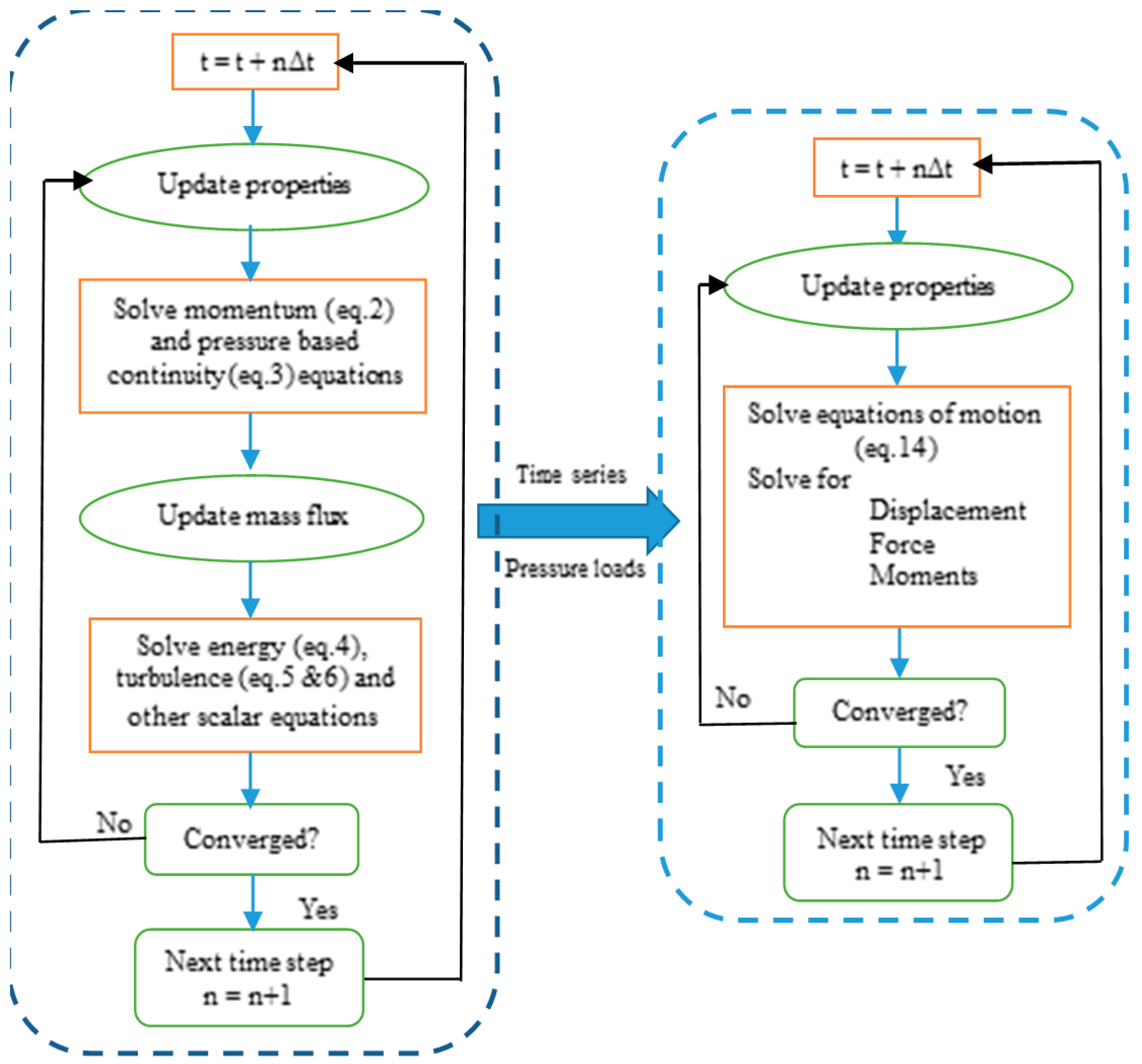
In the uni-directional FSI simulation, each solver runs separately and only the effect of one solver transfer to the other solver serves as the boundary or load condition, but not vice versa. In most cases, the CFD solves the aerodynamics to calculate the wind pressure on the blade, so that it will be applied to the structural solver (FE), but the effect of structural deformation on the fluid flow will not be considered (Figure 2). First, the fluid flow will be solved for each time step until the convergence criteria is attained; the pressure/force distribution calculated at the surface of the blade will be transferred to the structure side of the solver. Similarly, the structural dynamics will be solved until convergence is attained. This process will be repeated for each time step until the full study domain is covered. It is noteworthy to see that the displacement of the blade has no impact on the fluid flow, according to uni-directional coupling.
However, in bi-directional FSI, to capture the effect of structural deformation on aerodynamics, the deflection will be feedback to CFD and will improve the prior solution making a closed loop between the two solvers. The fluid solver will provide the forces acting on the blade and these forces will be transferred to the structural dynamics, and will be solved under the effect of these forces, resulting in nodal deformation. Unlike uni-directional coupling, the displacement at the boundary between the fluid and the blade will have to be transferred to the fluid field and interpolated as the fluid displacement. The fluid solver will be solved under the new configuration result in a new set of forces to be transferred to the structure solver. These steps will be repeated until the convergence criteria is attained, and the next time step will advance to cover the whole study domain. In addition, for bi-directional coupling, the mesh deformation at FSI boundary is critical, as it is the bridge to exchange whole information (force and displacement); therefore, either the conformal mesh method (which needs re-meshing or updating as the solution advances) or non-conformal mesh method (in which each solver works within their independent respective girds) can be incorporated, depending on the numerical constraints imposed. The latter method will be utilized for this specific work. The coupling algorithm for the two methods are shown below; uni-directional (Figure 2) and bi-directional (Figure 3).
3. Computational Model
The mathematical formulation in the previous section will be implemented using the Multiphysics package ANSYS (Version 16), each domain will be modeled in their respective solver and coupled according to coupling method selected, as stated below. The geometric copy of NREL 5-MW baseline wind turbine blade is considered [15,23], with certain amendments, refer Table 1. The two fluid-structure interaction models will be compared at the rated speed operation conditions of the turbine blade.
3.1. Computation Fluid Dynamics (CFD) Model
3.1.1. Computational Domain
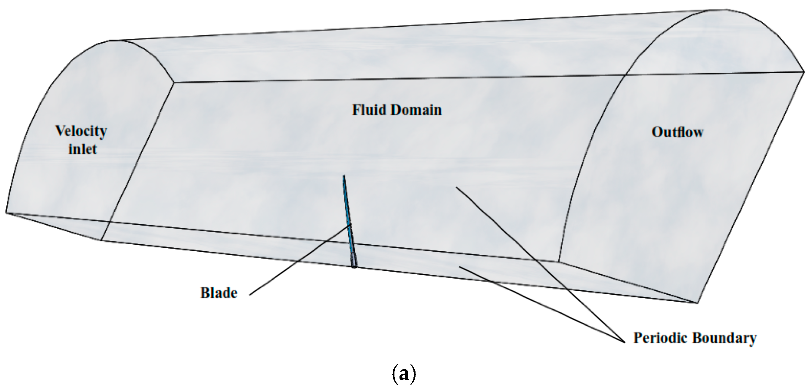
The aerodynamics of the blade is modeled on ANSYS Fluent, with a computational domain sized as shown in Figure 4a. The computational domain considered is a volume encompassed in a radius of 184.5 m and 123 m, and length of 246 m and 184.5 m at downwind and upwind of the blade, respectively. The wind turbine mode is symmetrical about its rotational axis; therefore, to reduce computational effort, periodic boundary will be utilized and 1/3rd of the full domain, i.e., only one blade and 1/3rd of the fluid domain is considered.
3.1.2. Solver Settings and Turbulence Model
As discussed in the previous section, the flow is considered as low Mach, incompressible flow, and therefore a pressure based coupled algorithm transient solver was chosen to solve the incompressible RANS equations.
A viscous flow with SST k-ω turbulence model is applied. It uses the ε-k turbulence model for the far filed part of the domain, and the ω-k turbulence model for the boundary layer. The convergence of the analysis is determined by using the residual monitor, and for the present study a residual value of 0.001 is set for continuity, velocity in three directions, turbulent kinetic energy and the specific dissipation rate, and 1 × 10⁻⁷ for the energy equation. The spatial discretization for pressure, momentum, turbulent kinetic energy and the specific dissipation and energy are all approximated to second order.
3.1.3. Boundary Conditions
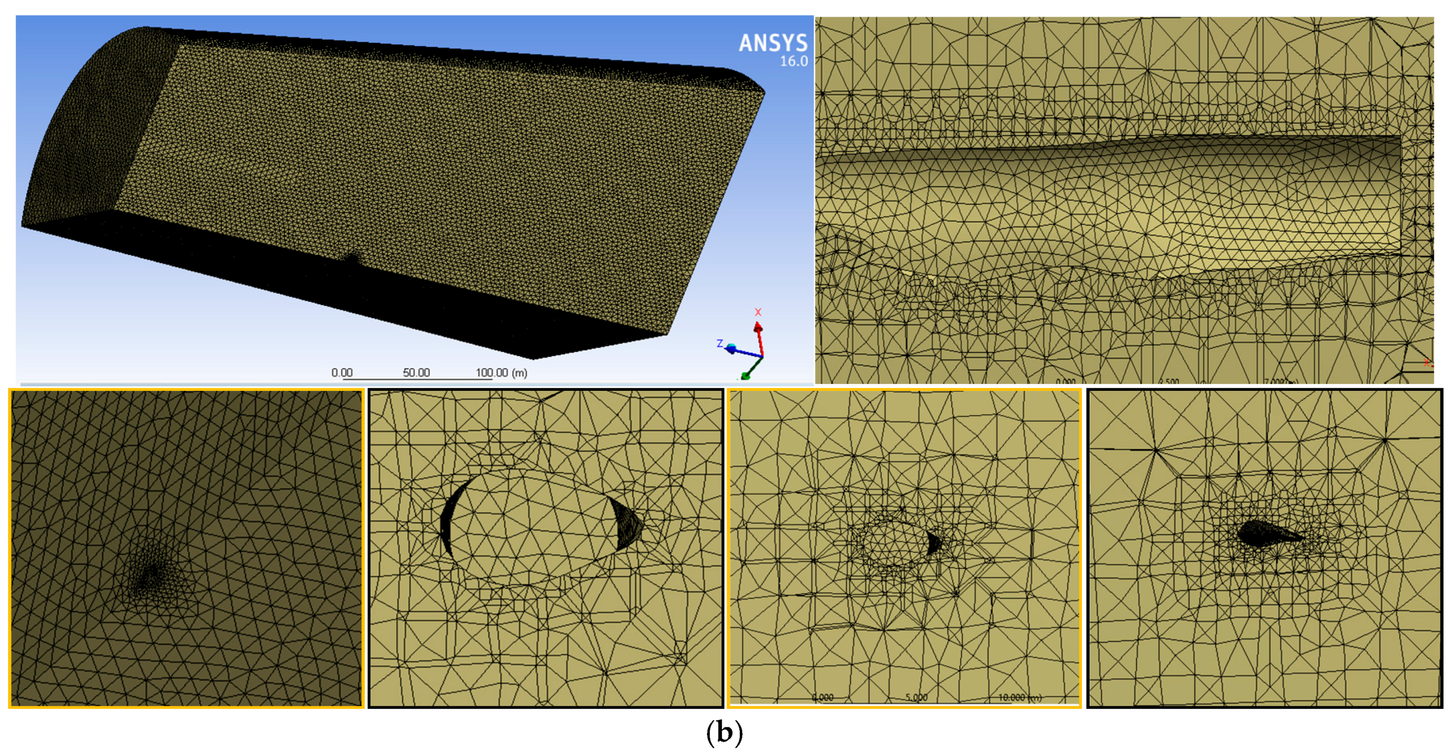
The upwind side of the wind turbine is modeled as velocity inlet with a free stream velocity of 11.4 m/s. Besides the upwind side of the wind turbine, the far field enclosing surface is modeled as velocity inlet boundary because of the tapered geometry along the flow direction. The downwind side is modeled as pressure outlet. The blade surface is a rotating wall with no slip shear condition, and it is a boundary between the fluid domain and the structural domain to transfer data among the two solvers as well. The domain is discretized with an unstructured grid, as shown in Figure 4b, and an extra inflation layer and finer meshes are applied at the blade surface to improve the resolution. The final computational grid includes 2.5 × 10⁶ elements encompassing 4.3 × 10⁵ nodes. Furthermore, only for bi-directional fluid structural coupling, dynamic mesh with re-meshing option has been applied to ensure system coupling and data exchange with the other solver.
3.2. Finite Element (FE) Model
3.2.1. Computational Domain
ANSYS transient structural module will be employed to investigate structural dynamics in response to the effect of wind flow. The target blade is a geometric copy of NREL 5MW baseline wind turbine blade [15,23] with 61.5 m length and cross-sectional distribution as described in Figure 5a and Table 1. At the root and the tip of the blade, certain amendments have been made to maintain smooth transformation from the cylindrical root to the first aerofoil, and an interpolation for chord and twist distribution at the tip portion, as per [24]. The geometry and aerodynamic property of the remaining aerofoils are kept similar as the reference blade.
3.2.2. Geometry and Material Distribution
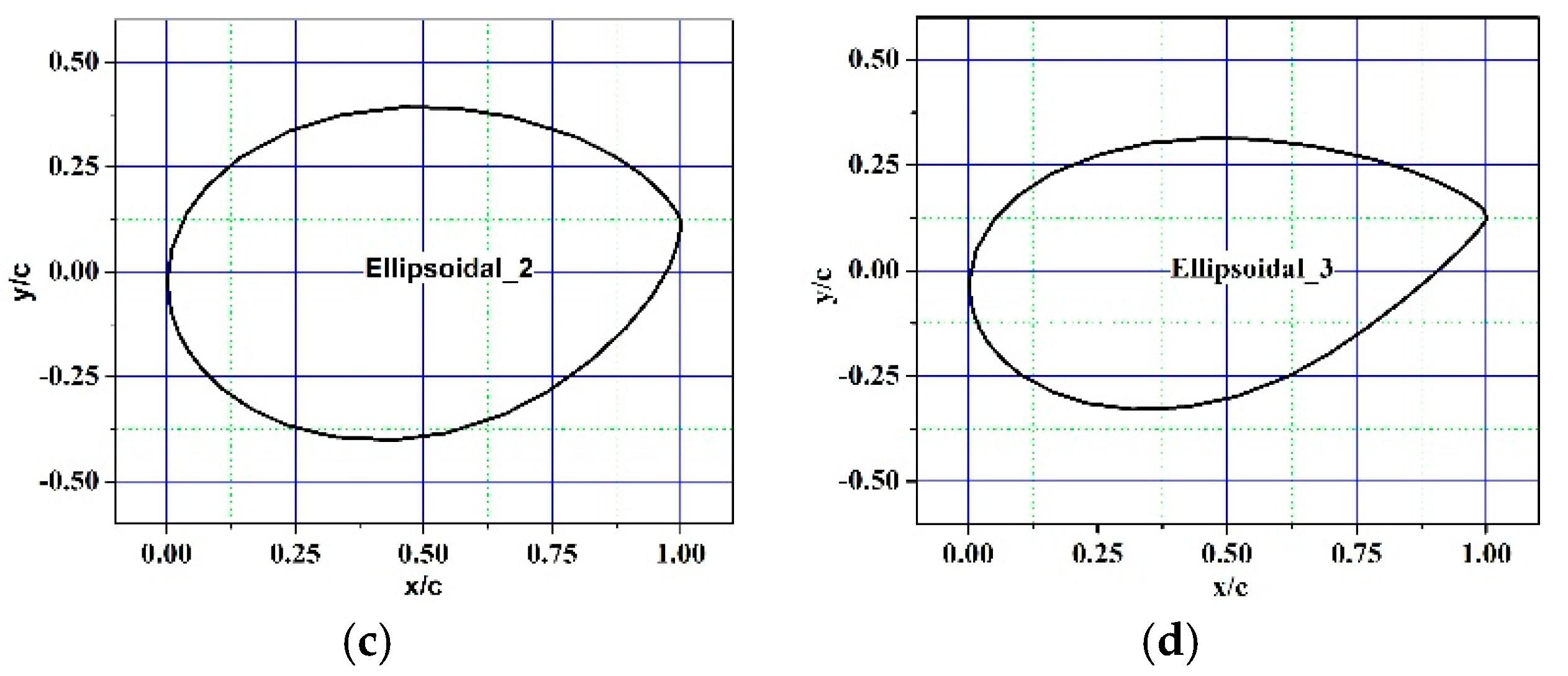
The structural model of the blade is composed of several components such as root, shell, priming, finish layer, spar cap, spar, and other structural adhesives, which are made of composite material layers. However, considering modeling difficulties and computation resources, for the present study the blade model is composed of only two major components: the aerodynamic surface enclosing the outermost area and the spars acting as a shear web. The material distribution is also simplified as the spars as Saertex/EP-3, and the rest of the blade as E-LT-5500/EP-3, with an orthotropic material property as shown in Table 2. The final FE model cross-sectional distributed properties of the blade along the span are as tabulated below (Table 1), and the modified root aerofoil shapes are as shown in Figure 6.
3.2.3. Boundary Conditions and Mesh
The 3D FE model of the blade developed with shell elements and discretized into 8.5 × 10⁴ elements comprised of 4.3 × 10⁴ nodes, Figure 5b. Further refinements are made at the blade surface as it is the coupling boundary to exchange aerodynamic forces and structural displacement, i.e., fluid-solid interface. A large deflection assumption is used, and remote displacement is applied as the blade root is eccentric from the center of rotation (with a radius of hub). The centrifugal forces are also considered by applying rotation velocity for the blade structure, i.e., rated blade velocity of 12.1 rpm.
3.3. Fluid-Structure Interaction Model
For the present study, uni-directional or one-way and bi-directional or two-way fluid-structure interaction models are considered, with the two models incorporated on ANSYS accordingly.
For the one-way model, the two solvers run separately. First, fluent solves the fluid domain and calculates the flow parameters such as the pressure distribution along the blade surface for the whole simulation time. Then, the transient structural solver receives the time series pressure distribution, calculates the aerodynamic force and determines the structural dynamics of the blade, such as stress and deflections.
For the two-way model, a system coupling model will be employed so that both solvers run simultaneously. The two solvers will exchange data (i.e., aerodynamic force from fluid solver to structural solver, and displacements from the structural solver to the fluid solver), after convergence is achieved at their respective domain. The iteration will continue until both solvers converge after data exchange.
3.4. Model Assessment
The CFD and FE models utilized in this study will be evaluated and validated as follows. As presented in the previous section, the structural property of the FE blade model is slightly different than the reference NREL 5MW baseline blade (refer Table 1, Table 2 and Table 3).
Therefore, significant differences in dynamic responses are expected. In the following section, the justification of the models (both CFD and FE) will be addressed.
3.4.1. CFD Model
The CFD model utilized will be validated against results from NREL FAST code for NREL 5MW wind turbine, and also by monitoring some of the flow parameters such as mass imbalance during the simulation.
In evaluating the mass imbalance for both FSI models between the inlet and outlet, the net imbalance is calculated to be 0.10900877 kg/s and −0.34917137 kg/s for uni-directional and bi-directional FSI model, respectively (Table 4). In both models, the imbalance is negligible.
Another validation parameter considered is the power curve. For the present article, the rated operational condition is the primary study domain; therefore, the power developed at the rated speed will be calculated for both coupling models and compared with reference rated power, i.e., 5 MW [15]. The power developed by the wind turbine system is given by:
where: : rotation speed, , : blade aerodynamic torque, and : drivetrain efficiency, [25]. The blade aerodynamic torque is the sum of the edgewise moment of each blade. From the simulation result, the mean edgewise moment for a single blade is calculated to be −1.47 × 10⁷ Nm for one-way coupling and −1.58 × 10⁷ Nm for the two-way coupling model. Note that the edgewise moment calculated for a single blade should be multiplied by three to match the reference turbine. Therefore, based on Equation (16), the rated power is calculated to be −51.7 MW and −53.6 MW for uni-directional and bi-directional models. Comparing these values with the reference value of 5 MW [15], a large difference is recorded. This difference arises due to the simplification of the structural model and the assumptions in the flow domain such as no wind shear, zero pitch angle and angle of attack.
3.4.2. FE Model
In the present study, the fluid structure interaction of the wind turbine is studied using the geometric copy of the NREL 5MW wind turbine blade. The dynamics of a single blade is used to compare the performance of the two FSI models, i.e., uni-directional and bi-directional models. The FE model hence will be validated using modal analysis. To validate the FE model utilized, a reliable modal test result for a single blade with the same structural configuration is required; to the authors’ knowledge, there is no reliable modal analysis result for a single blade of the NREL 5MW baseline wind turbine. In relation to NREL 5MW wind turbine modal parameters, the available data from [15,23,26,27] can be considered. However, most of the available data for modal parameters of the NREL 5MW turbine are the results of a full-system analysis, including the blades, drivetrain, nacelle, and tower. With the application of Multi Blade Coordinate Transformation, the individual modes of each blade are transformed into the whole rotor mode [27], i.e., the first flapwise modes of each blade are summed up to be the first Asymmetric Flapwise Yaw, Asymmetric Flapwise Pitch, and Collective Flapwise mode of the rotor, including the coupling with the nacelle-yaw and nacelle pitching motions [15]. Based on the modal analysis of the FE model, the first five mode shapes of the blade structure are depicted in Figure 7, including the first to third flapwise mode shapes and the first and second edgewise mode shapes.
The modal frequency of the FE model of the blade is also presented in Figure 8. To validate the current result, the modal frequency of a 62.7 m long blade from [28] is plotted with it. The two blades have similar aerofoil distributions [15,28], with some differences such as pre-bended blade in [6] but pre-coned blade in [15] and a 1.2 m length difference. Assessing Figure 8 and the modal frequencies for each mode, the frequencies of the FE model and LMH64-5 blade are closer for the 1st, 2nd and 4th mode but a significant difference is seen in the third mode, i.e., the 2nd flapwise mode.
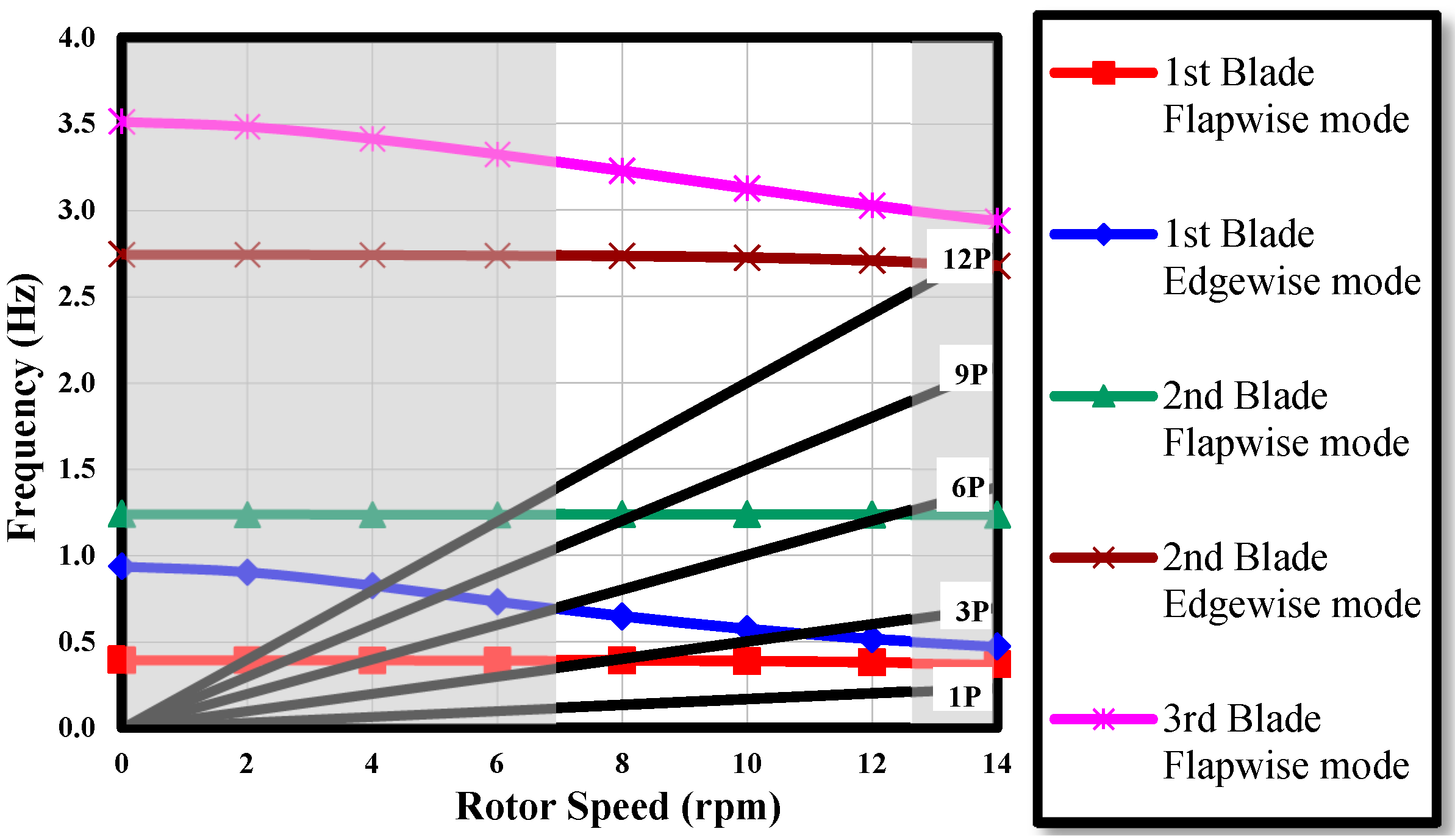
Another justification for the FE model can be drawn from the Campbell diagram of the blade given at Figure 9; the trend of the modal frequency with the rotor speed can be fairly considered to be similar to the reference blade [26].
Evaluating the above justifications and comparing the FSI results with the theoretical backgrounds, both the CFD and FE model of the wind turbine blade employed in this article can be fairly considered valid to compare the two FSI (uni-directional and bi-directional) models. In the following sections, the results of the two FSI model will be studied and compared.
4. Results and Discussion
Based on the models and methodologies presented in the previous section, the two fluid-structural interaction models (i.e., unidirectional and bi-directional) are assessed and compared. The results are categorized as aerodynamic and structural response.
4.1. Aerodynamic Responses
Both coupling methods showed that the pressure distribution along the blade span tends to increase from the root to the tip (Figure 10). However, due to blade deformation in bi-directional coupling, the designed angle of attack in the flow domain was altered (Figure 11b) and a slight difference recorded in contrast to uni-directional coupling (Figure 11a).
The pressure and velocity contour can be more illustrative of the influence of blade deformation on the aerodynamic response. The pressure contour on the blade surface for both coupling models is depicted in Figure 11.
Comparison of velocity and pressure contour at four locations along the blade span viz. 0.15 R, 0.3 R, 0.6 R, and 0.9 R are considered as well (Figure 12 and Figure 13). The magnitude of pressure and velocity in bi-directional coupling excels its counterpart more significantly at the mid portion of the blade.
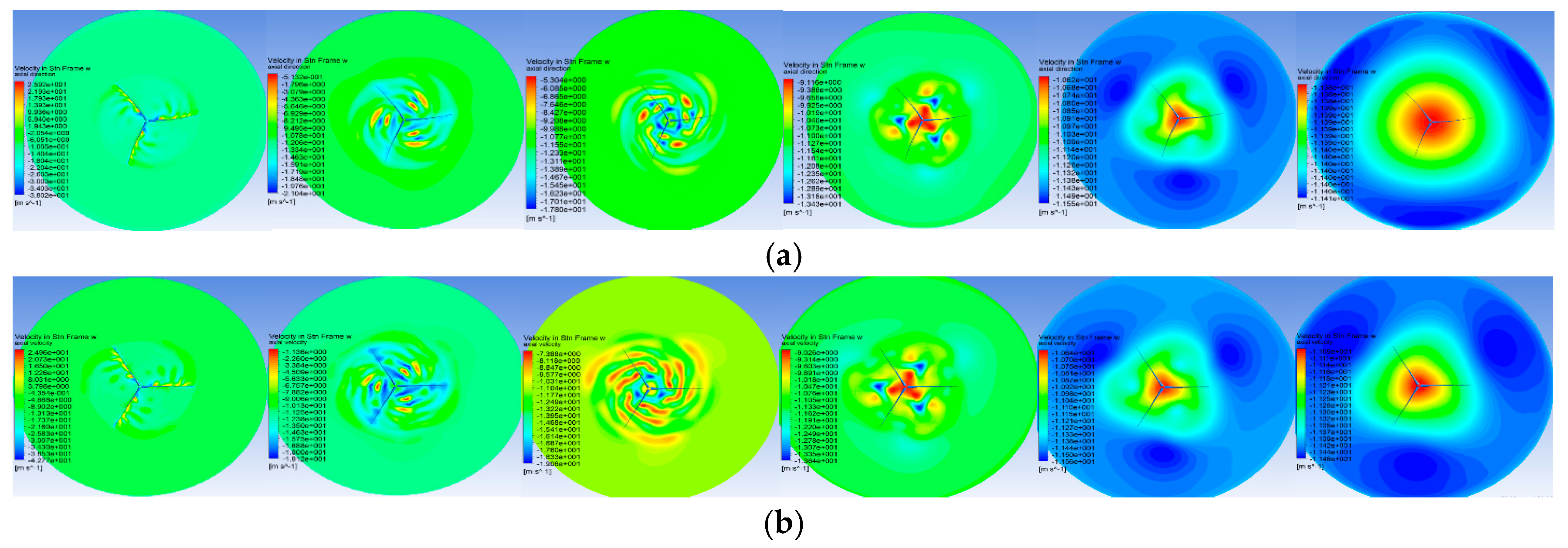
Furthermore, the effect of fluid structure coupling can also be pronounced by the flow pattern across the flow domain, and it seems to alter the pressure and velocity gradient, tip vortex, and downwind wake pattern (Figure 14).
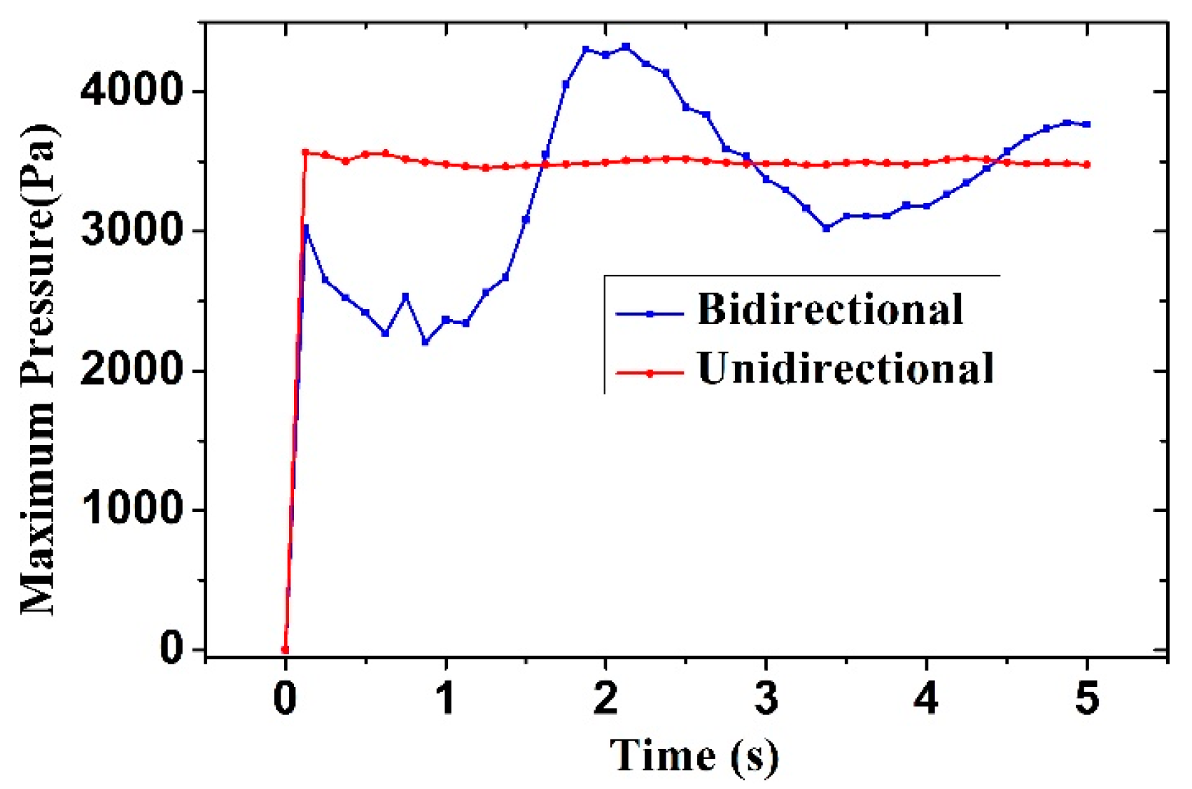
The maximum pressure variation with time across the blade is further evidence for the influence of blade deformation on the flow parameters (Figure 15). In the uni-directional model, a maximum pressure of 3.5 MPa is achieved faster and maintained, while in the bi-directional model, it fluctuates harmonically.
4.2. Structural Response
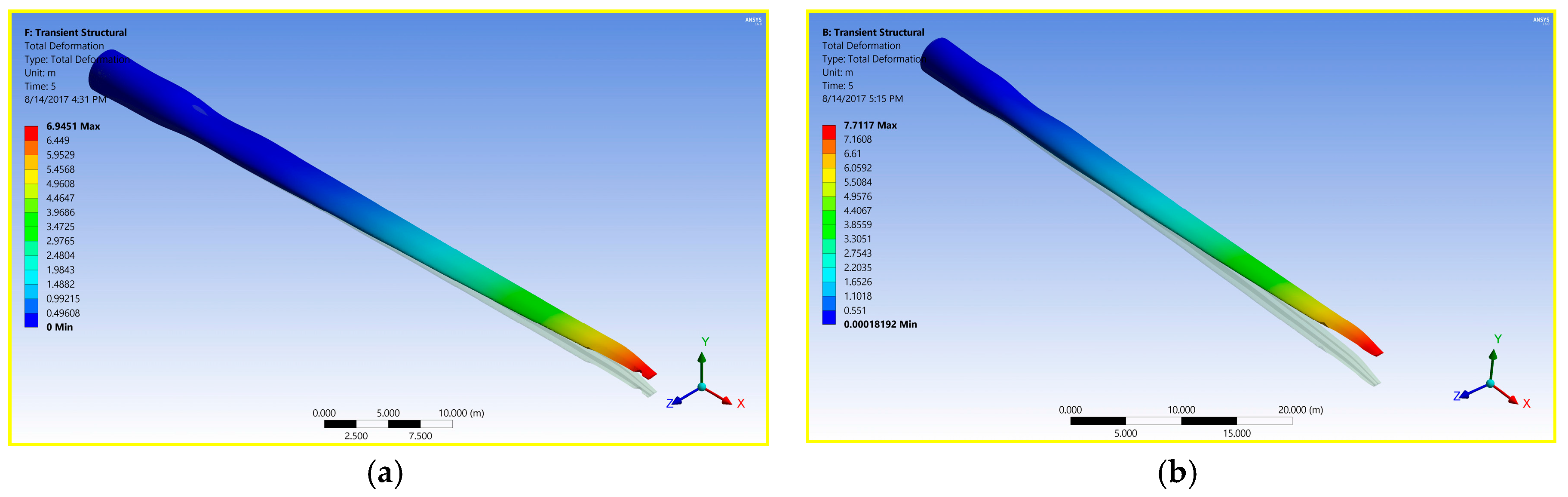
The structural dynamic of the blade is also affected by the fluid structural coupling methods, as the pressure distribution (Figure 15) is changing with time so as the blade deflection (Figure 16). For uni-directional coupling, the deflections tend to stabilize; however, as for bi-directional coupling, even though the amplitude is decreasing, there is still significant vibration and deformation variation. The structural dynamics of the blade are also affected by the fluid structural coupling models utilized; the total blade deformation at the end of 5 s is depicted in Figure 17. In both models, the deflection increases from the root to the tip; however, the magnitude in the bi-directional model is larger.
In relation to pressure and blade deformation variation, the output power is also affected, as the edgewise root moment is fluctuating (Figure 18). The edgewise moment for bi-directional coupling is 180 degrees out of phase with the tip deflection and varies inversely, and by extension, the output power of the blade will fluctuate as the deflection affects the flow pattern.
Furthermore, besides the variation of power output, the structural loading is also affected by the FSI model used, as shown in Figure 19 and Figure 20. From the equivalent von-mises stress contour at the suction and pressure side of the blade, one should notice the difference in stress concentration locations for the two coupling methods. In bi-directional coupling, the root of the blade is a highly stressed location with a magnitude of 368 MPa (Figure 19b); conversely, the leading edge is the most stressed part of the blade in uni-directional coupling with a maximum of 330 MPa (Figure 19a).
5. Conclusions
This paper presents an extensive comparison between uni-directional and bi-directional fluid structure interaction models, using a geometric copy of the NREL 5MW wind turbine blade at the rated wind speed of 11.4 m/s. In bi-directional coupling, the originally designed angle of attack altered due to blade deflection, as did the aerodynamic performance and by extension the structural dynamics, while the uni-directional coupling failed to pronounce such phenomena.
- The pressure on the blade, the total tip deflection and the blade root moments in the uni-directional model fluctuates for one second and maintains a constant value; however, in the bi-directional model the fluctuation continues.
- Comparing the tip vortex and the axial velocity gradient along the downwind side of the blade, the free stream velocity was attained faster in the bi-direction model than the uni-directional model.
- In the bi-directional model, the root of the blade is a highly stressed location with a magnitude of 368 MPa, and the leading edge is the most stressed part of the blade in the uni-directional model with a maximum of 330 MPa. In relation, the power developed would also fluctuate in the bi-directional model whereas it would have a constant value in the bi-directional coupling model.
It is observed that the bi-directional model is more natural and reliable to model the fluid-structure interaction of the wind turbine. In multi-MW wind turbines with flexible and thin blades, the fluid-structure interaction is very tight and influential, hence strong bi-directional coupling can provide more credible results and insights than uni-directional coupling. However, enormous computation resources are required; in this regard, the uni-directional model could be a possible alternative for preliminary design and load forecasting. The computation effort limitation related to full tightly coupled FSI can be reduced with a certain fidelity compromise, using reduced models and hybrid solvers (zonal hybrid) for the individual solver, applying optimal grid size, using simplified geometry and material distribution.
Acknowledgments
This work was financially supported by the China Government Scholarship Program. The authors also would like to acknowledge Wuhan University of Technology for providing holistic assistance in the course of the study.
Author Contributions
Mesfin Belayneh Ageze ran and post-processed the complete set of simulation for both FSI models, analyzed the results, and wrote the manuscript. Yefa Hu and Huachun Wu analyzed the simulation results and revised the manuscript. All authors read and approved the final manuscript.
Conflicts of Interest
All authors declare no conflict of interest.
References
- International Energy Agency. Long-Term Research and Development Needs for Wind Energy for the Time Frame 2012 to 2030; International Energy Agency: Paris, France, 2013. [Google Scholar]
- Tabassum, A.; Premalatha, M.; Abbasi, T.; Abbasi, S.A. Wind energy: Increasing deployment, rising environmental concerns. Renew. Sustain. Energy Rev. 2014, 31, 270–288. [Google Scholar] [CrossRef]
- Ageze, M.; Hu, Y.; Wu, H. Wind Turbine Aeroelastic Modeling: Basics and Cutting Edge Trends. Int. J. Aerosp. Eng. 2017, 2017, 5263897. [Google Scholar] [CrossRef]
- Hou, G.; Wang, J.; Layton, A. Numerical Methods for Fluid-Structure-Review. Commun. Comput. Phys. 2012, 12, 337–377. [Google Scholar] [CrossRef]
- Marshall, J.G.; Imregun, M. A review of aeroelasticity methods with emphasis on turbomachinery applications. J. Fluids Struct. 1996, 10, 237–267. [Google Scholar] [CrossRef]
- Carrión, M.; Steijl, R.; Woodgate, M.; Barakos, G.N.; Munduate, X.; Gomez-Iradi, S. Aeroelastic analysis of wind turbines using a tightly coupled CFD–CSD. J. Fluids Struct. 2014, 50, 392–415. [Google Scholar] [CrossRef]
- Hirt, C.W.; Amsden, A.A.; Cook, J.L. An Arbitrary Lagrangian–Eulerian Computing Method for All Flow Speeds. J. Comput. Phys. 1997, 135, 203–216. [Google Scholar] [CrossRef]
- Hu, H.H.; Patankar, N.A.; Zhu, M.Y. Direct Numerical Simulations of Fluid–Solid Systems Using the Arbitrary Lagrangian–Eulerian Technique. J. Comput. Phys. 2001, 169, 427–462. [Google Scholar] [CrossRef]
- Yuri, B.; Takizawa, K.; Tezduyar, T.E.; Hsu, M.; Kostov, N.; McIntyre, S. Aerodynamic and FSI Analysis of Wind Turbines with the ALE-VMS and ST-VMS Methods. Arch. Comput. Methods Eng. 2014, 21, 359–398. [Google Scholar]
- Tian, F.; Wang, Y.; Young, J.; Lai, J.C.S. An FSI solution technique based on the DSD/SST method and its applications. Math. Models Methods Appl. Sci. 2015, 25, 2257–2285. [Google Scholar] [CrossRef]
- Tian, F.-B. FSI modeling with the DSD/SST method for the fluid and finite difference method for the structure. Comput. Mech. 2014, 54, 581–589. [Google Scholar] [CrossRef]
- Benra, F.; Dohmen, H.J.; Pei, J.; Schuster, S.; Wan, B. A Comparison of One-Way and Two-Way Coupling Methods for Numerical Analysis of Fluid-Structure Interactions. J. Appl. Math. 2011, 2011, 853560. [Google Scholar] [CrossRef]
- Chen, Y.; Wang, Z.; Tsai, G. Two-way Fluid-Structure Interaction Simulation of a Micro Horizontal Axis Wind Turbine. Int. J. Eng. Technol. Innov. 2015, 5, 33–44. [Google Scholar]
- Kumar, J.; Wurm, F. Bi-directional fluid-structure interaction for large deformation of layered composite propeller blades. J. Fluids Struct. 2015, 57, 32–48. [Google Scholar] [CrossRef]
- Jonkman, J.; Butterfield, S.; Musial, W.; Scott, G. Definition of a 5-Mw Reference Wind Turbine for Offshore System Development; Technical Report NREL/TP-500-38060; National Renewable Energy Laboratory: Golden, CO, USA, 2009.
- Hansen, M.; Sørensen, J.; Voutsinas, S.; Sørensen, N.; Madsen, H. State of the art in wind turbine aerodynamics and aeroelasticitys. Prog. Aerosp. Sci. 2006, 42, 285–330. [Google Scholar] [CrossRef]
- Menter, F.R. Two-equation eddy-viscosity turbulence models for engineering applications. AIAA J. 1994, 32, 1598–1605. [Google Scholar] [CrossRef]
- Villalpando, F.; Reggio, M.; Ilinca, A. Assessment of Turbulence Models for Flow Simulation around a Wind Turbine Airfoil. Model. Simul. Eng. 2011, 2011, 714146. [Google Scholar] [CrossRef]
- Menter, F.R. Zonal two-equation model k–w models for aerodynamic flows. In Proceedings of the 23rd Fluid Dynamics, Plasmadynamics, and Lasers Conference, Orlando, FL, USA, 6–9 July 1993. [Google Scholar]
- Hodges, D.H.; Dowell, E.H. Nonlinear Equations of Motion for the Elastic Bending and Torsion of Twisted Nonuniform Rotor Blades; National Aeronautics and Space Administration: Washington, DC, USA, 1974.
- Kaza, K. Nonlinear Aeroelastic Equations of Motion of Twisted, Nonuniform, Flexible Horizontal-Axis Wind Turbine Blades; Toledo University: Toledo, OH, USA, 1980. [Google Scholar]
- Kallesøe, B.S. Equations of motion for a rotor blade, including gravity, pitch action and rotor speed variations. Wind Energy 2007, 10, 209–230. [Google Scholar] [CrossRef]
- Kooijman, H.J.T.; Lindenburg, C.; Winkelaar, D.; van der Hooft, E.L. Dowec 6 MW Pre-Design: Aero-Elastic Modelling of the DOWEC 6 MW Pre-Design in Phatas; ECN Wind Energy: Amsterdam, The Netherland, 2003. [Google Scholar]
- Martin, H.R. Development of a Scale Model Wind Turbine for Testing of Offshore Floating Wind Turbine Systems; The University of Maine: Orono, ME, USA, 2011. [Google Scholar]
- Griffin, D. WindPACT Turbine Design Scaling Studies Technical Area 1-Composite Blades for 80- to 120-Meter Rotor; National Renewable Energy Laboratory: Golden, CO, USA, 2001.
- Jonkman, J.M.; Jonkman, B.J. FAST modularization framework for wind turbine simulation: Full-system linearization. J. Phys. Conf. Ser. 2016, 753. [Google Scholar] [CrossRef]
- Stol, K.A.; Moll, H.G.; Bir, G.; Namik, H. A Comparison of Multi-Blade Coordinate Transformation and Direct Periodic Techniques for Wind Turbine Control Design. In Proceedings of the 47th AIAA Aerospace Sciences Meeting Including the New Horizons Forum and Aerospace Exposition, Orlando, FL, USA, 5–8 January 2009. [Google Scholar]
- Lindenburg, C. Aeroelastic Modelling of the LMH64–5; Energy Research Centre of the Netherlands: Petten, The Netherlands, 2002. [Google Scholar]
- Bir, G.; Jonkman, J. Aeroelastic Instabilities of Large Offshore and Onshore Wind Turbines. J. Phys. Conf. Ser. 2007, 75. [Google Scholar] [CrossRef]
Figure 1.
(a) Coordinate frames (3D); and (b) blade cross-section. Note: : section coordinate, : pitching moment, : elastic twisting deflection, : are the aerodynamic forces.
Figure 1.
(a) Coordinate frames (3D); and (b) blade cross-section. Note: : section coordinate, : pitching moment, : elastic twisting deflection, : are the aerodynamic forces.
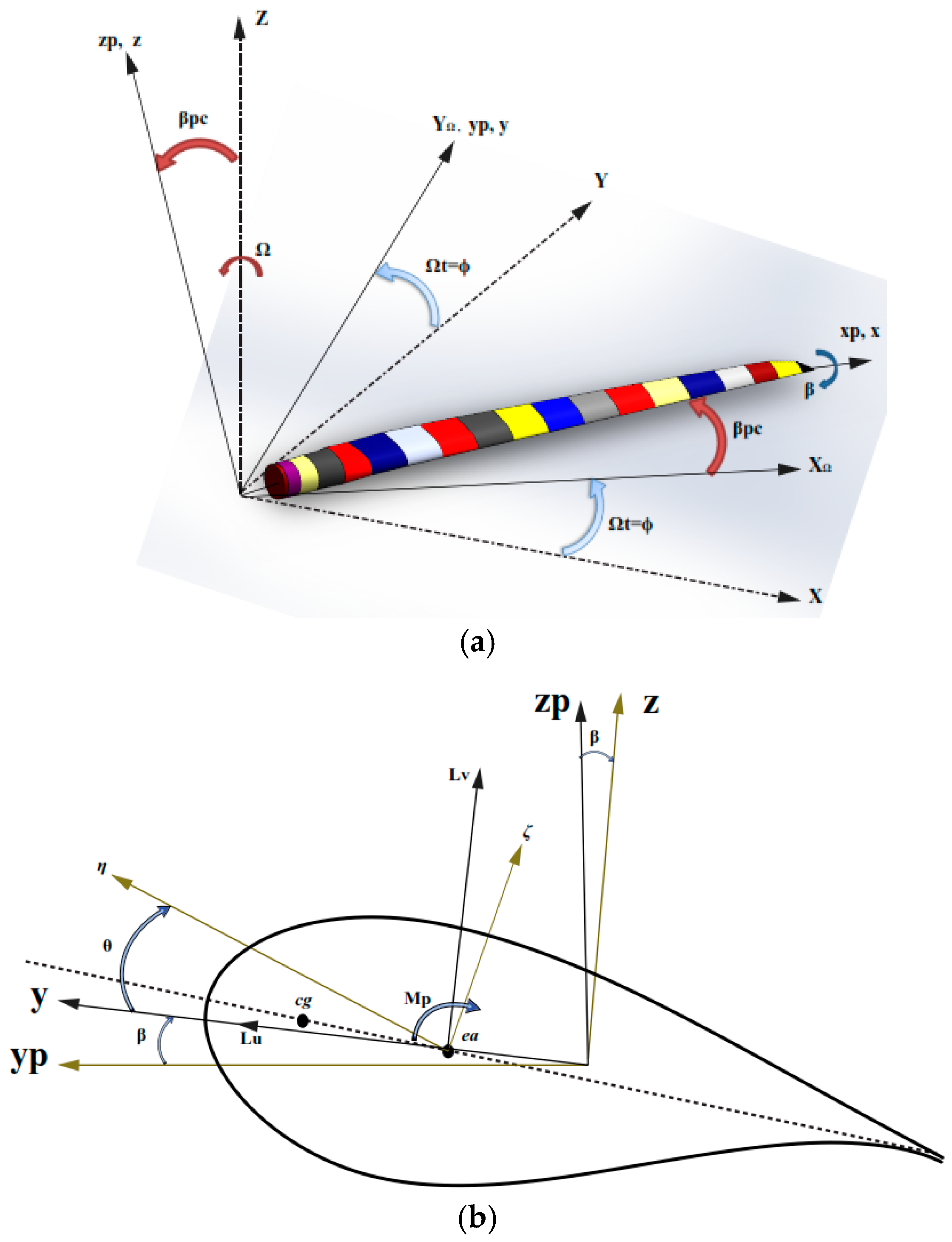
Figure 2.
Uni-directional fluid structure coupling algorithm.

Figure 3.
Bi-directional fluid structure coupling algorithm.
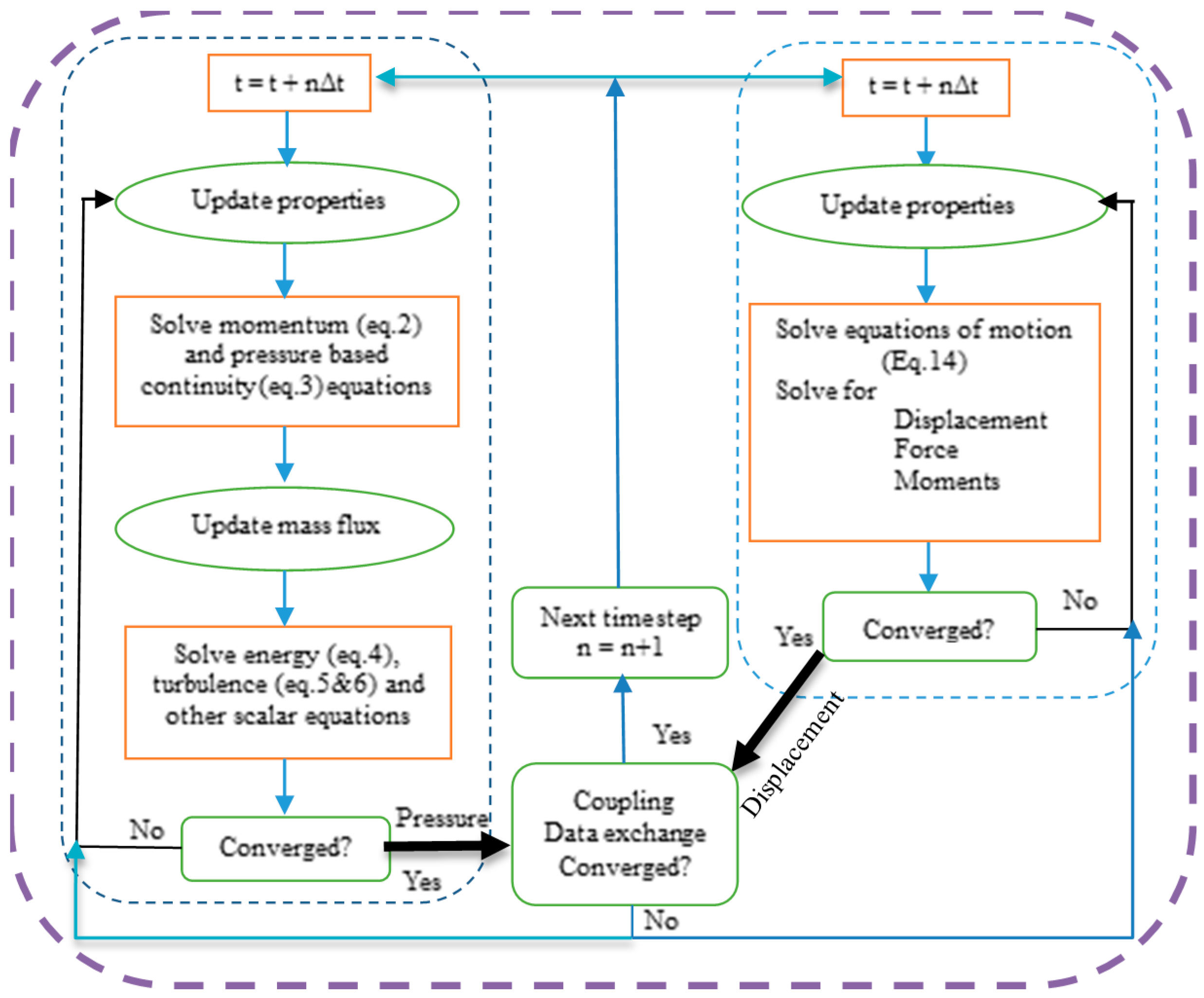
Figure 4.
(a) Computational domain with boundary conditions and (b) meshes for the fluid domain.


Figure 5.
Aerofoil distribution along the blade span (a) and mesh (b) for the structural domain.
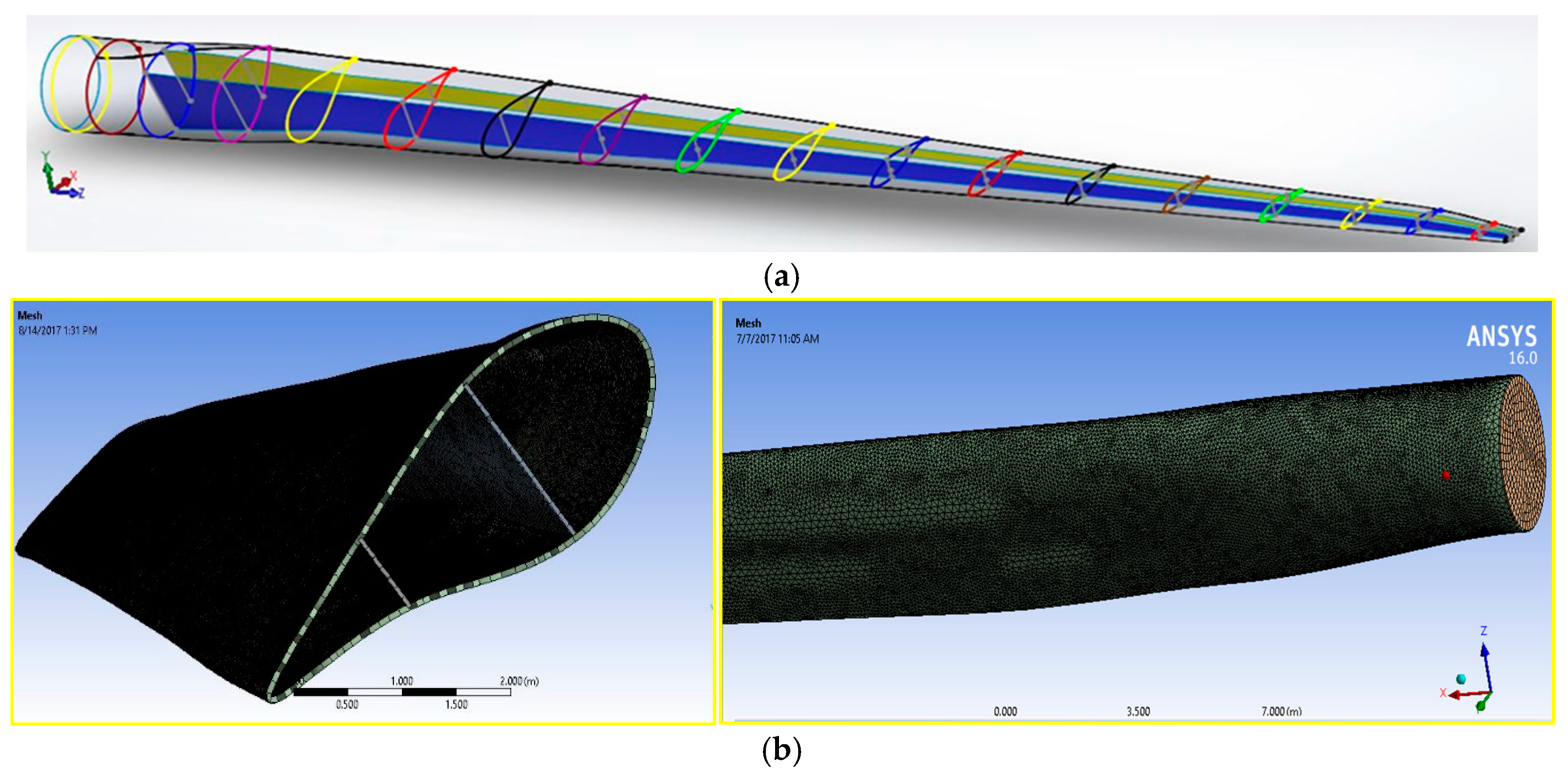
Figure 6.
Root aerofoil geometry, from blade root to tip in the order of (a–d), respectively.
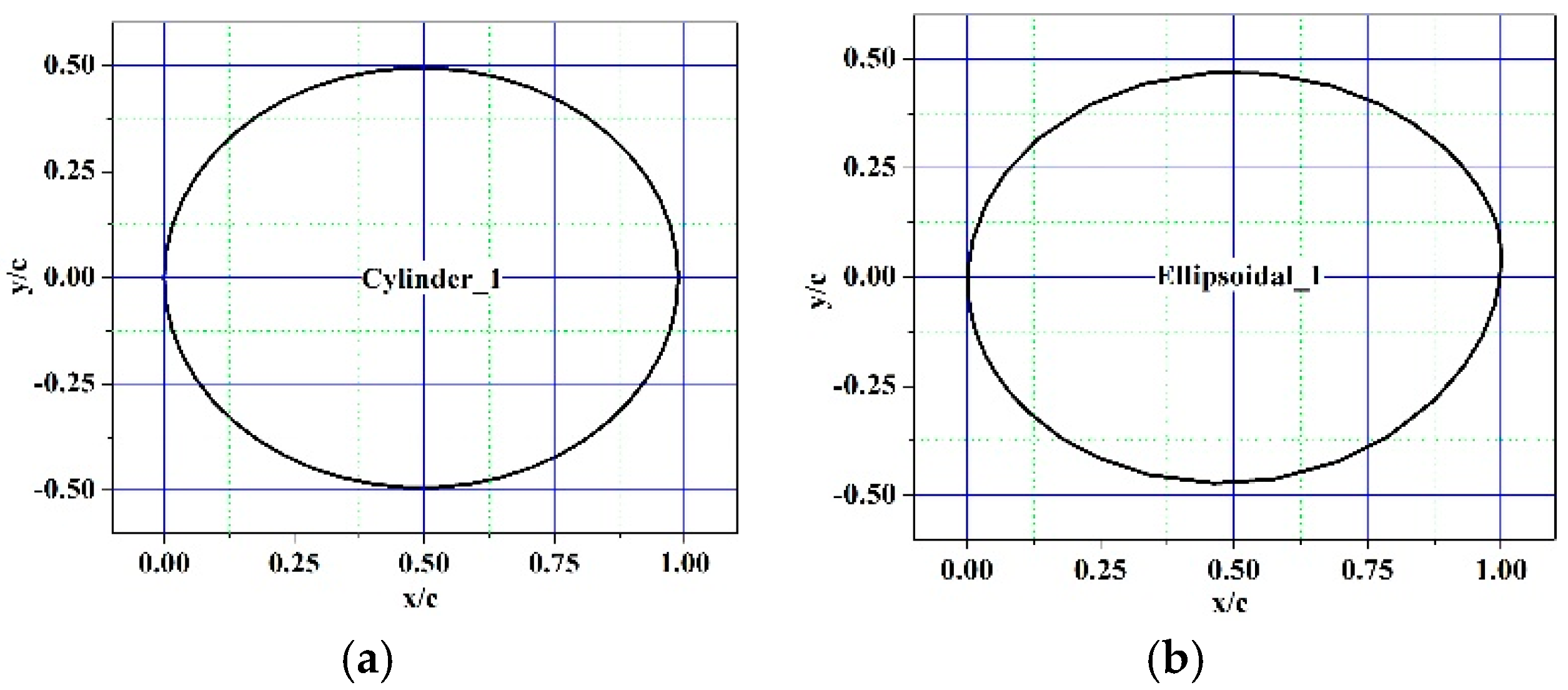

Figure 7.
Modal shape of the blade, (a–d) the 1st, 2nd and 3rd flapwise modes, and (b,e) the 1st and 2nd edgewise modes.
Figure 7.
Modal shape of the blade, (a–d) the 1st, 2nd and 3rd flapwise modes, and (b,e) the 1st and 2nd edgewise modes.
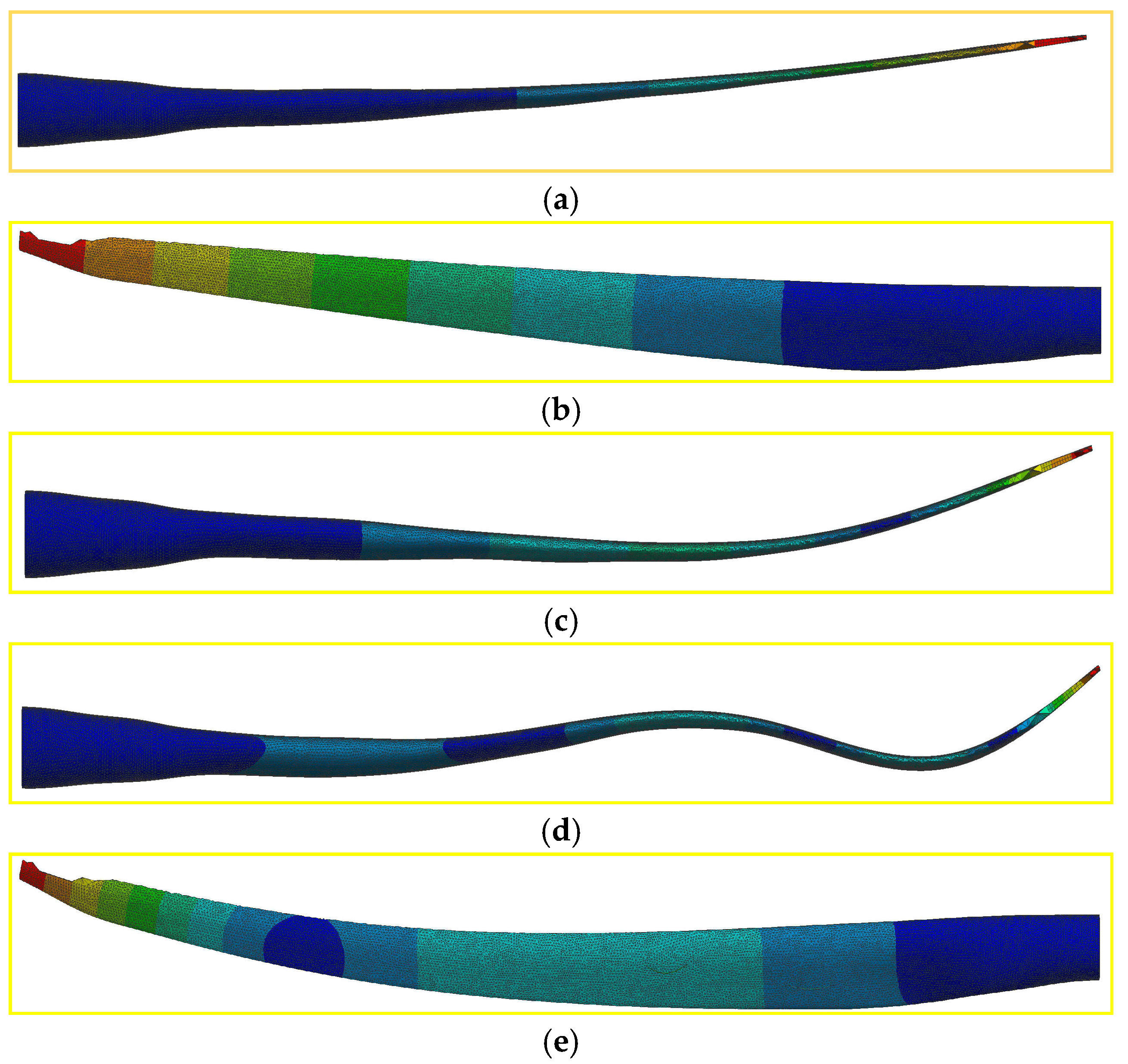
Figure 8.
The 1st five modal frequency of the blade (FE mode) and the 1st four “reactionless” modal frequency of LMH64-5 blade [29] at 12.1 rpm.
Figure 8.
The 1st five modal frequency of the blade (FE mode) and the 1st four “reactionless” modal frequency of LMH64-5 blade [29] at 12.1 rpm.
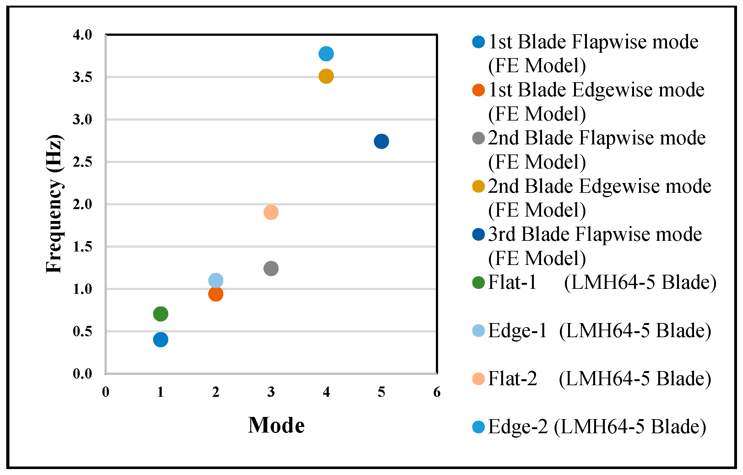
Figure 9.
Campbell diagram of the blade (FE model).

Figure 10.
Maximum pressure along the blade span at the end of the first cycle, i.e., 5-s simulation.
Figure 10.
Maximum pressure along the blade span at the end of the first cycle, i.e., 5-s simulation.
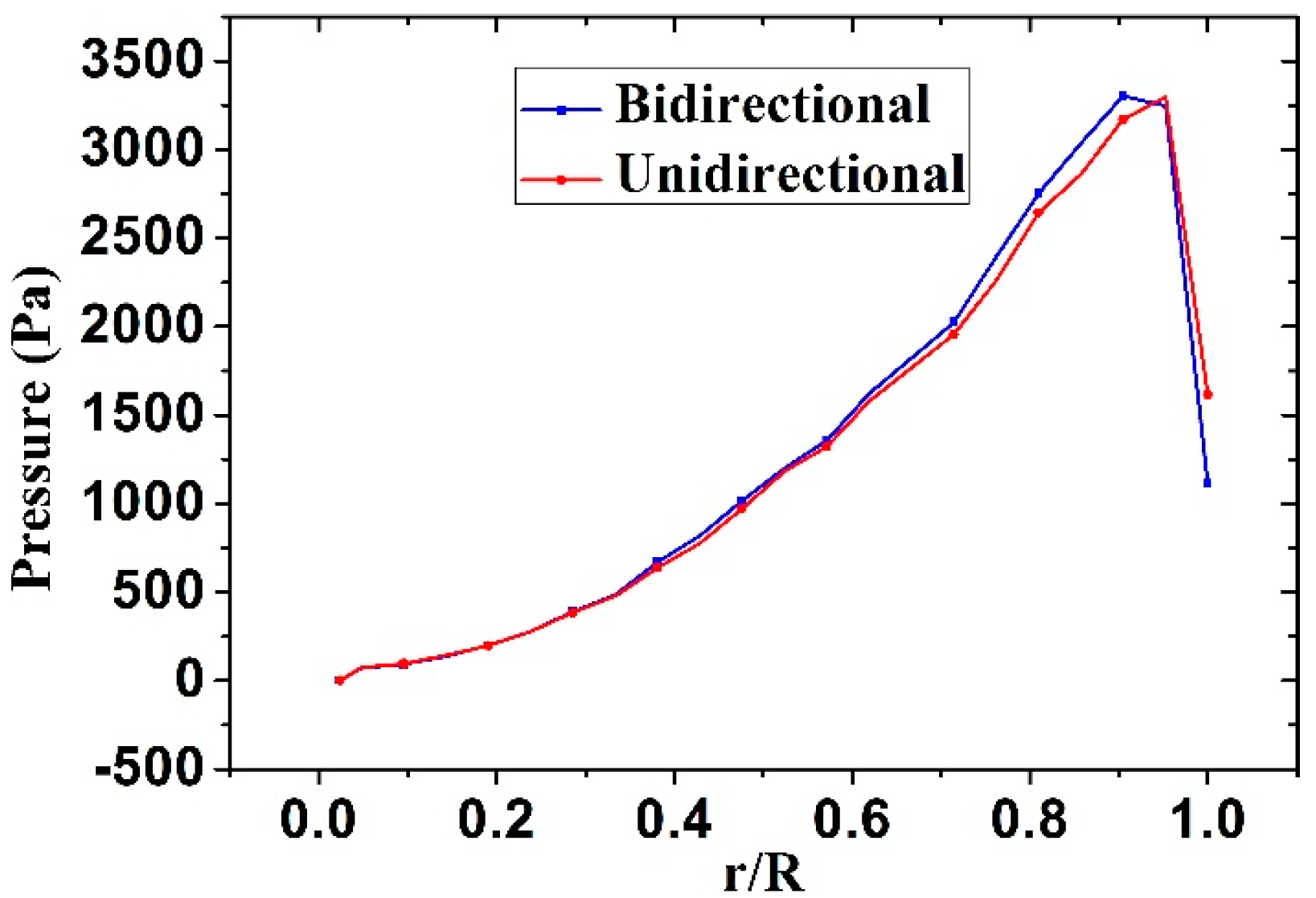
Figure 11.
Pressure contour (a) uni-directional and (b) bi-directional at the 5th second of the simulation.
Figure 11.
Pressure contour (a) uni-directional and (b) bi-directional at the 5th second of the simulation.
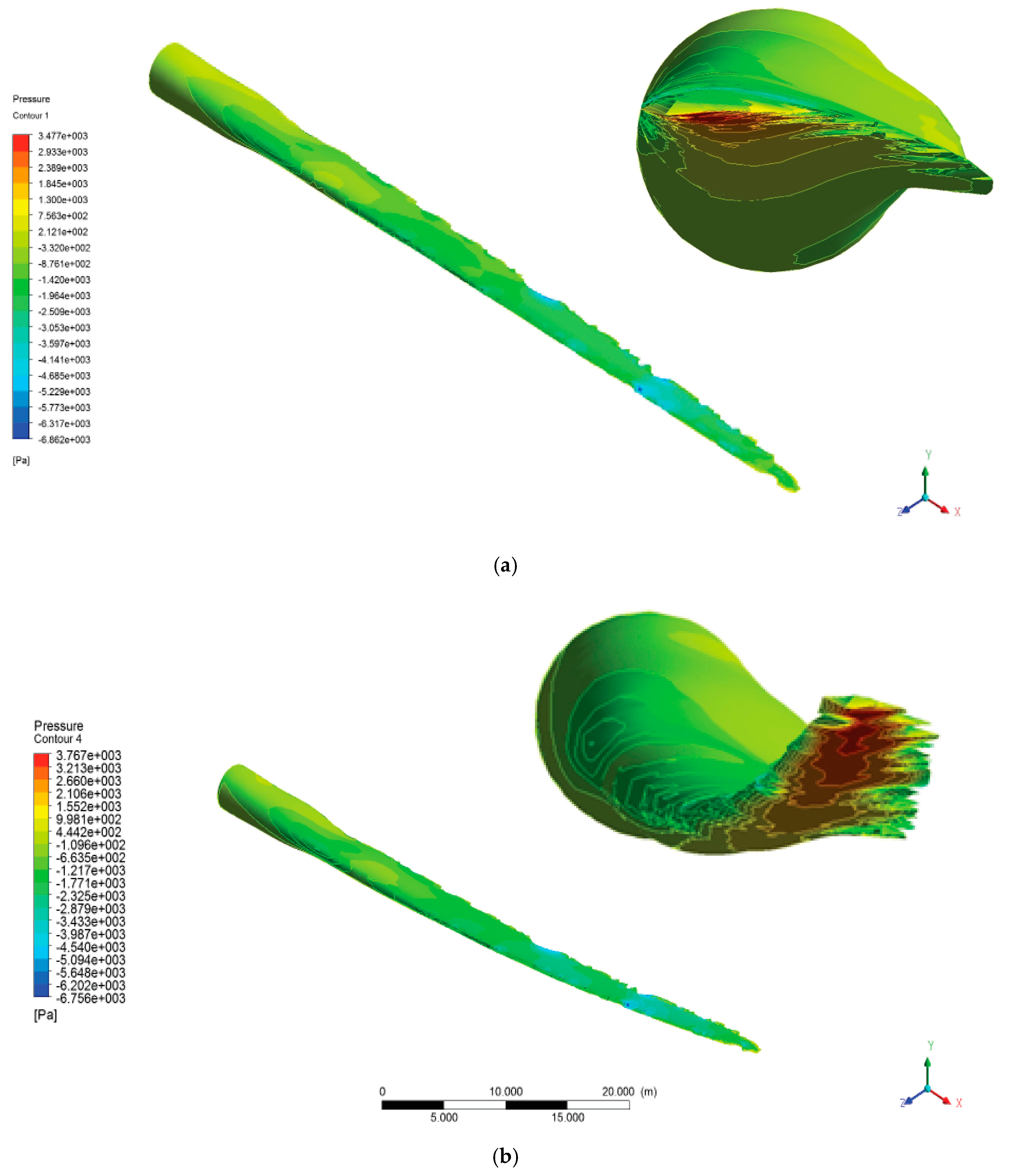
Figure 12.
Velocity contour, uni-directional (a) and bi-directional (b) coupling at the end of 5 s.
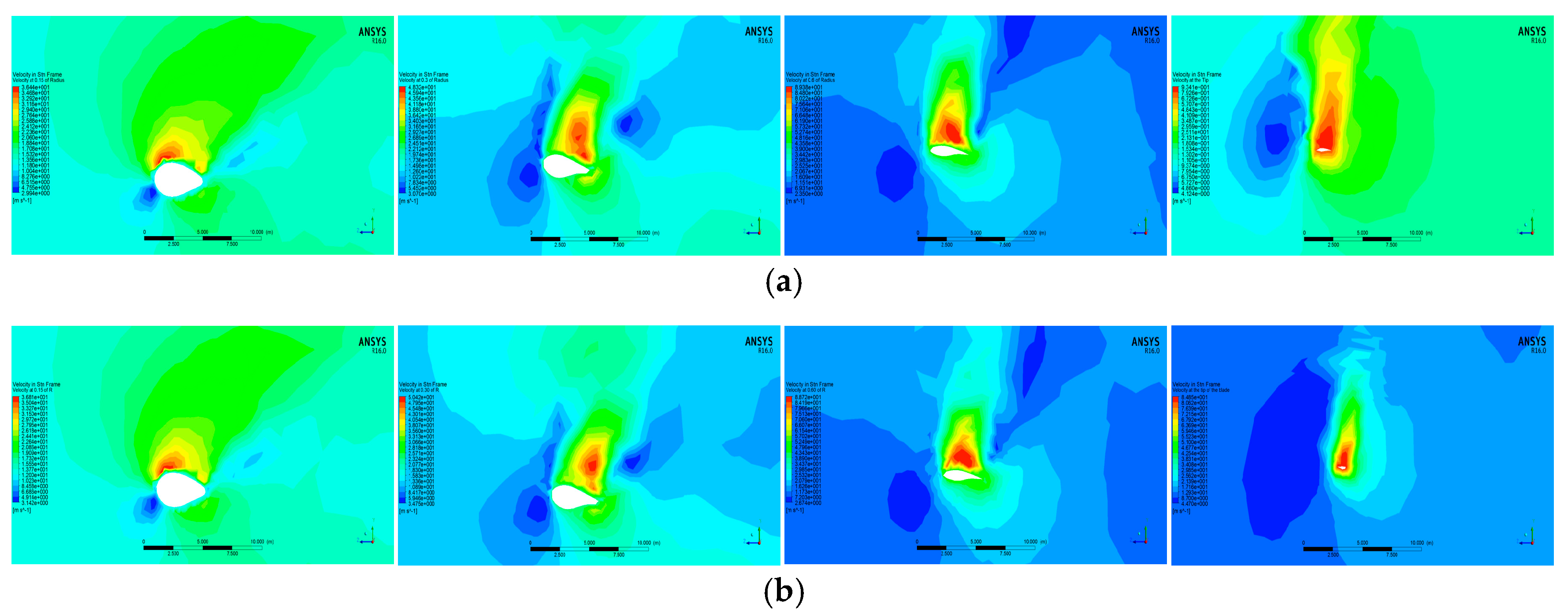
Figure 13.
Pressure contour, (a) uni-directional; and (b) bi-directional coupling at the end of 5 s.
Figure 13.
Pressure contour, (a) uni-directional; and (b) bi-directional coupling at the end of 5 s.
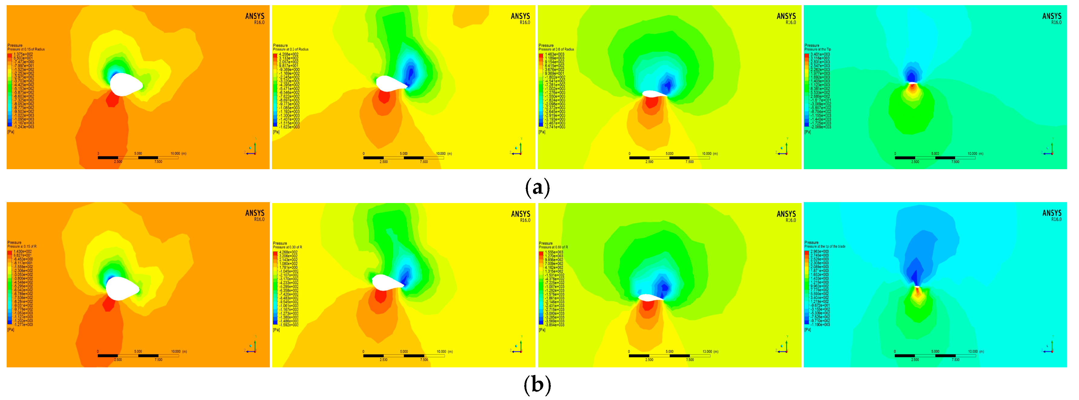
Figure 14.
Axial velocity contour along the downwind direction (at 0, 10, 20, 60, 80, and 200 m behind the blade, left to right, respectively), (a) bi-directional; and (b)uni-directional.
Figure 14.
Axial velocity contour along the downwind direction (at 0, 10, 20, 60, 80, and 200 m behind the blade, left to right, respectively), (a) bi-directional; and (b)uni-directional.

Figure 15.
Maximum pressure variation with time.

Figure 16.
(a) Edgewise; (b) Flapwise; and (c) Total tip deflection at rated speed.
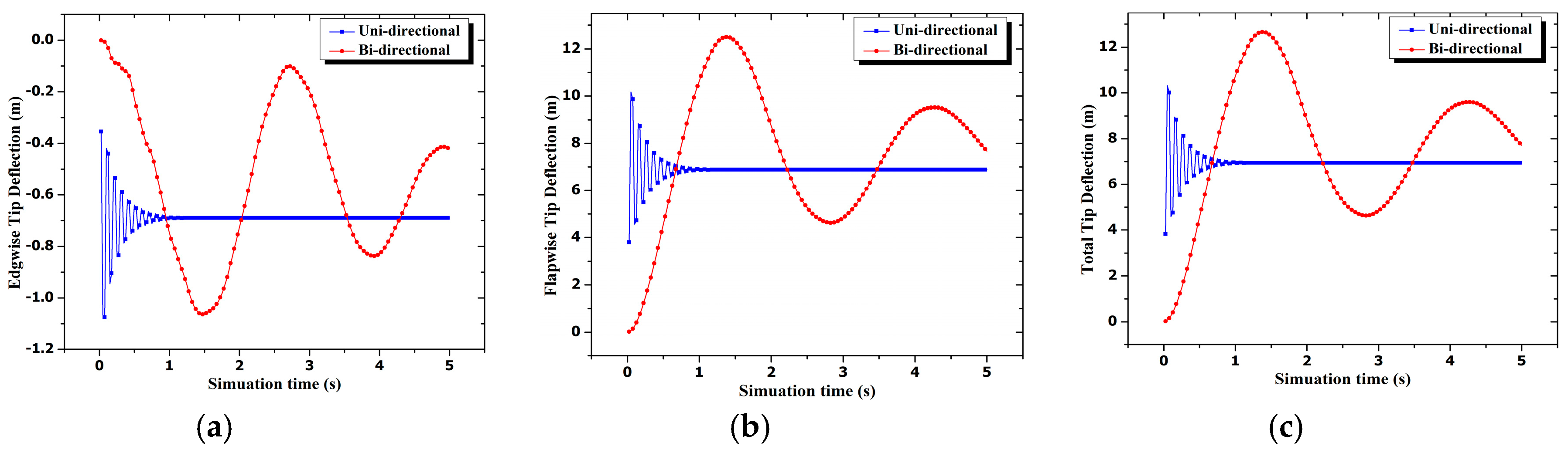
Figure 17.
Total blade deformation; (a)uni-directional, and (b)bi-directional, at the end of 5 s.

Figure 18.
(a) Edgewise moment; and (b) Flapwise moment variation with time at rated speed.
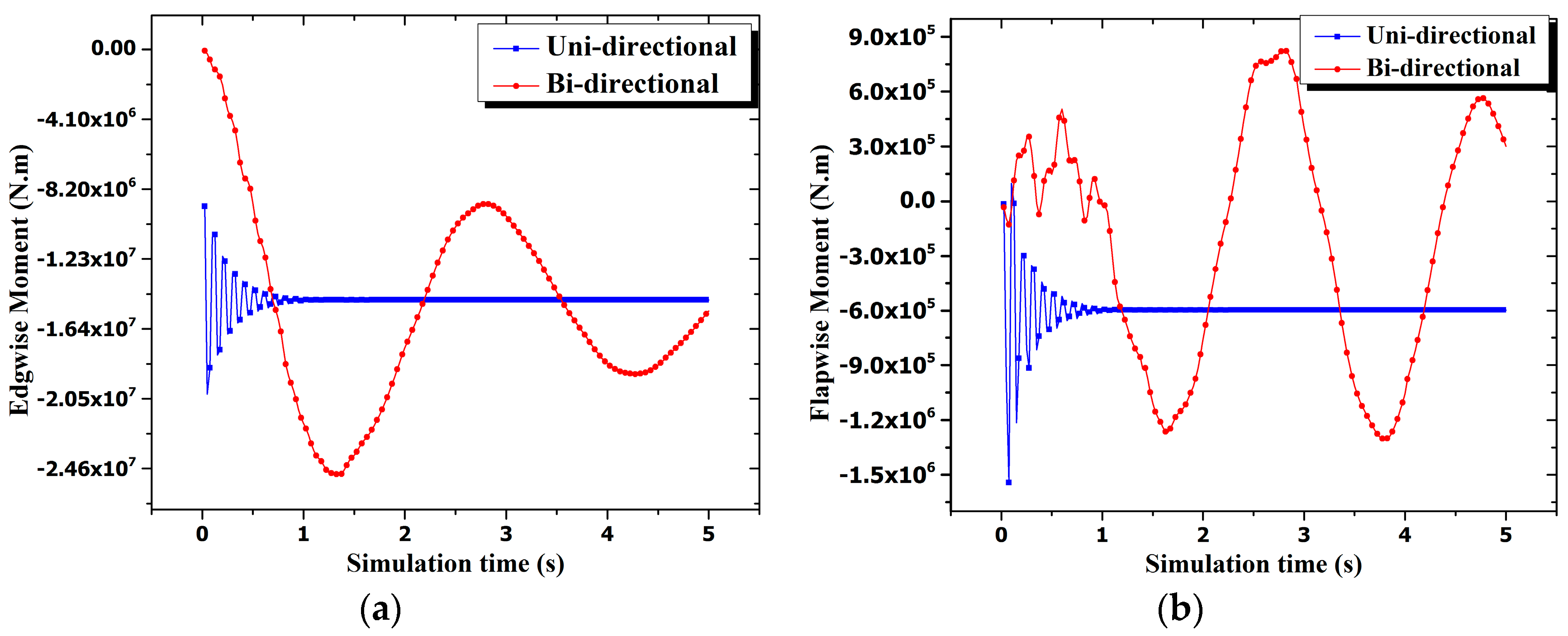
Figure 19.
Von-mises stress contour at the end of 5 s; (a) uni-directional; and (b) bi-directional.
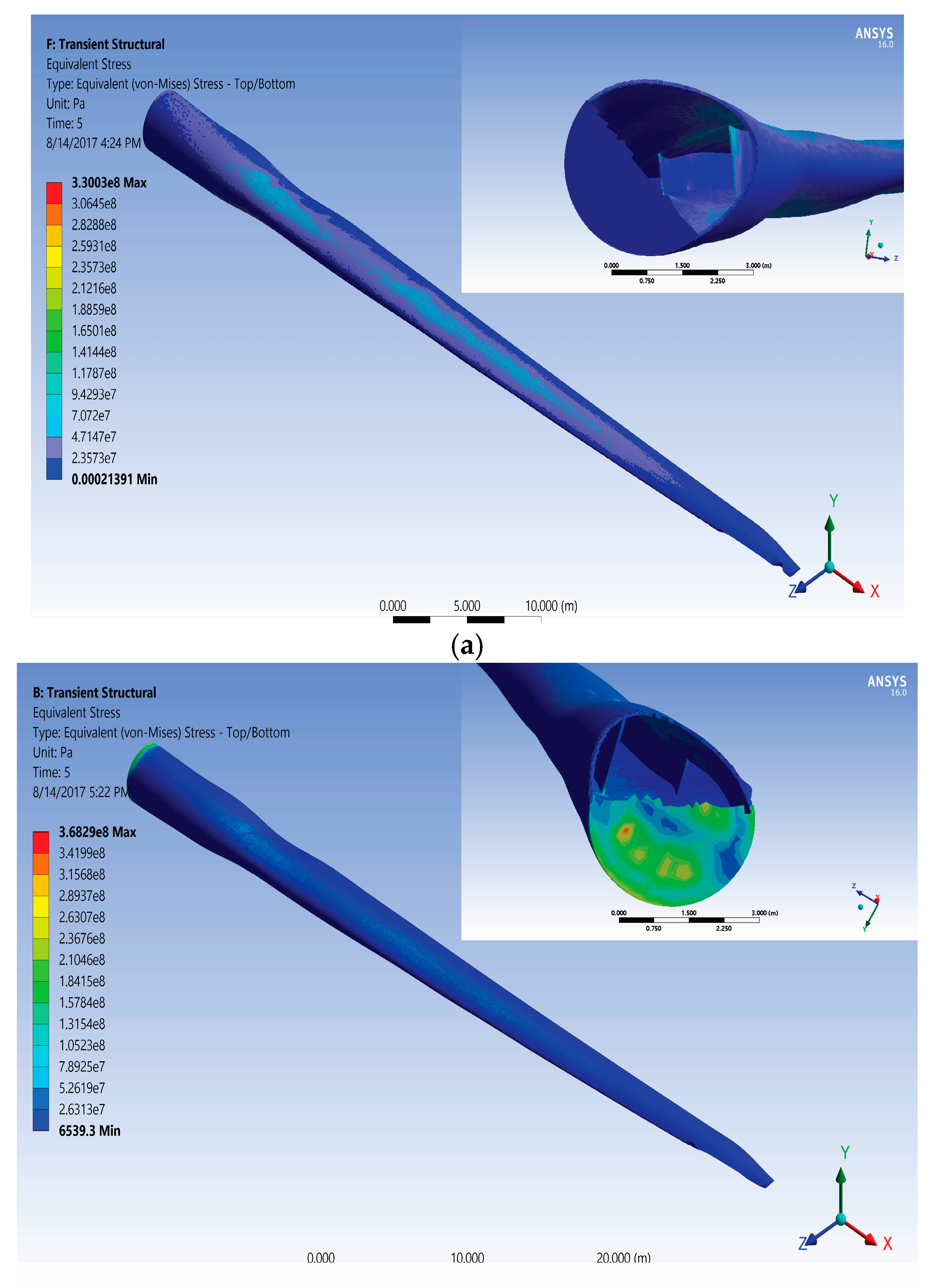
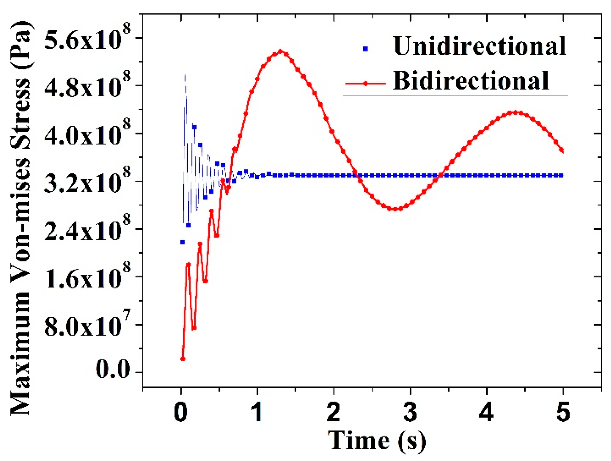
Figure 20.
Maximum equivalent von-mises stress variation with time.

Table 1.
Sectional properties of the blade.
| Station No. ** | Radius | Aerofoil | Chord (m) | Twist (°) | Principal Moment of Inertia at the Section Centroid | Solid Cross-Sectional Area (m2) | Section Centroid (m) * | ||
|---|---|---|---|---|---|---|---|---|---|
| IXX (m4) | IYY (m4) | J (m4) | |||||||
| 1 | 1.5000 | Cyclinder1 | 3.5420 | 13.3080 | 1.05 | 1.07 | 2.12 | 0.671 | (1.7, 0.402, 1.5) |
| 2 | 1.9530 | Cyclinder1 | 3.5420 | 13.3080 | 1.04 | 1.07 | 2.11 | 0.668 | (1.7, 0.402, 1.95) |
| 3 | 3.4020 | Ellipsoidal_1 | 3.5726 | 13.3080 | 0.96 | 1.06 | 2.02 | 0.651 | (1.73, 0.416, 3.4) |
| 4 | 5.5440 | Ellipsoidal_2 | 3.8060 | 13.3080 | 0.951 | 1.24 | 2.19 | 0.959 | (1.8, 0.448, 5.54) |
| 5 | 8.6330 | Ellipsoidal_3 | 4.0997 | 13.3080 | 0.626 | 1.27 | 1.9 | 0.874 | (1.89, 0.502, 8.63) |
| 6 | 11.7500 | DU40_A17 | 4.5570 | 13.3080 | 0.27 | 1.23 | 1.5 | 0.728 | (2.05, 0.486, 11.7) |
| 7 | 15.8500 | DU35_A17 | 4.6520 | 11.4800 | 0.179 | 1.2 | 1.37 | 0.675 | (2.13, 0.413, 15.9) |
| 8 | 19.9500 | DU35_A17 | 4.4580 | 10.1620 | 0.15 | 1.0 | 1.15 | 0.617 | (2.05, 0.349, 19.9) |
| 9 | 24.0500 | DU30_A17 | 4.2490 | 9.0110 | 0.103 | 0.771 | 0.873 | 0.528 | (2, 0.309, 24.1) |
| 10 | 28.1500 | DU25_A17 | 4.0070 | 7.7950 | 0.0528 | 0.601 | 0.653 | 0.458 | (1.9, 0.3, 28.1) |
| 11 | 32.2500 | DU25_A17 | 3.7480 | 6.5440 | 0.0411 | 0.466 | 0.507 | 0.406 | (1.79, 0.241,32.3) |
| 12 | 36.3500 | DU21_A17 | 3.5020 | 5.3610 | 0.0229 | 0.35 | 0.373 | 0.347 | (1.68, 0.223,36.4) |
| 13 | 40.4500 | DU21_A17 | 3.2560 | 4.1880 | 0.0171 | 0.265 | 0.282 | 0.304 | (1.57, 0.176, 40.5) |
| 14 | 44.5500 | NACA64_A17 | 3.0100 | 3.1250 | 0.00884 | 0.191 | 0.2 | 0.256 | (1.46, 0.15, 44.6) |
| 15 | 48.6500 | NACA64_A17 | 2.7640 | 2.3190 | 0.00648 | 0.138 | 0.145 | 0.219 | (1.34, 0.119, 48.6) |
| 16 | 52.7500 | NACA64_A17 | 2.5180 | 1.5260 | 0.00462 | 0.0973 | 0.102 | 0.186 | (1.22, 0.091, 52.7) |
| 17 | 56.1667 | NACA64_A17 | 2.3130 | 0.8630 | 0.00338 | 0.0708 | 0.0742 | 0.16 | (1.12, 0.0704, 56.2) |
| 18 | 58.9000 | NACA64_A17 | 2.0860 | 0.3700 | 0.00237 | 0.0493 | 0.0517 | 0.137 | (1.01, 0.0543, 58.9) |
| 19 | 61.6333 | NACA64_A17 | 1.4190 | 0.1060 | 0.000773 | 0.0149 | 0.0157 | 0.088 | (0.691, 0.0332, 61.6) |
| 20 | 63 | NACA64_A17 | 1.0870 | 0 | 0.000368 | 0.00663 | 0.007 | 0.0658 | (0.529, 0.0233, 63) |
* With reference coordinate passing through the leading edge of the blade and starting from the center of the rotor, ** Station No. refers to the cross-section of the blade at the given radius from the center of the hub.
Table 2.
Material properties.
| Material | Lay-up | EL(GPa) | ET(GPa) | GLT(GPa) | Poisson’s Ratio (νLT) | Density (kg/m3) |
|---|---|---|---|---|---|---|
| E-LT-5500/EP-3 | 0 | 41.8 | 14 | 2.63 | 0.28 | 1920 |
| Saertex/EP-3 | 45 | 13.6 | 13.3 | 11.8 | 0.51 | 1780 |
Table 3.
Comparison of blade FE model and NREL 5MW baseline blade.
| Properties | NREL 5MW | FE Model |
|---|---|---|
| Length (w.r.t. Root Along Preconed Axis) | 61.5 m | 61.5 m |
| Overall (Integrated) Mass | 17,740 kg | 48,122 kg |
| CM Location (w.r.t. Root along Preconed Axis) | 20.475 m | 23.397 m |
| Pre-cone | 2.5° | 0 |
Table 4.
Mass imbalance of the two models.
| Sub-Domain | Mass Flow Rate (kg/s) | |
|---|---|---|
| Uni-Directional | Bi-Directional | |
| Inlet | 232,138.22 | 232,138.22 |
| Inlet top (far field ) | 265,637.39 | 265,637.39 |
| Outlet | −497,775.5 | −497,775.96 |
| Net | 0.10900877 | −0.34917137 |
© 2017 by the authors. Licensee MDPI, Basel, Switzerland. This article is an open access article distributed under the terms and conditions of the Creative Commons Attribution (CC BY) license (http://creativecommons.org/licenses/by/4.0/).
Share and Cite
MDPI and ACS Style
Ageze, M.B.; Hu, Y.; Wu, H. Comparative Study on Uni- and Bi-Directional Fluid Structure Coupling of Wind Turbine Blades. Energies 2017, 10, 1499. https://doi.org/10.3390/en10101499
AMA Style
Ageze MB, Hu Y, Wu H. Comparative Study on Uni- and Bi-Directional Fluid Structure Coupling of Wind Turbine Blades. Energies. 2017; 10(10):1499. https://doi.org/10.3390/en10101499
Chicago/Turabian StyleAgeze, Mesfin Belayneh, Yefa Hu, and Huachun Wu. 2017. "Comparative Study on Uni- and Bi-Directional Fluid Structure Coupling of Wind Turbine Blades" Energies 10, no. 10: 1499. https://doi.org/10.3390/en10101499
Note that from the first issue of 2016, this journal uses article numbers instead of page numbers. See further details here.