Development and Experimental Validation of a TRNSYS Dynamic Tool for Design and Energy Optimization of Ground Source Heat Pump Systems

Abstract

Ground source heat pump (GSHP) systems stand for an efficient technology for renewable heating and cooling in buildings. To optimize not only the design but also the operation of the system, a complete dynamic model becomes a highly useful tool, since it allows testing any design modifications and different optimization strategies without actually implementing them at the experimental facility. Usually, this type of systems presents strong dynamic operating conditions. Therefore, the model should be able to predict not only the steady-state behavior of the system but also the short-term response. This paper presents a complete GSHP system model based on an experimental facility, located at Universitat Politècnica de València. The installation was constructed in the framework of a European collaborative project with title GeoCool. The model, developed in TRNSYS, has been validated against experimental data, and it accurately predicts both the short- and long-term behavior of the system.

1. Introduction

Ground source heat pump (GSHP) systems represent an efficient and comfortable alternative for the air conditioning of any kind of space [1]. In this kind of systems, the ground is used as a heat source in winter and as a heat sink in summer, which provides a notable increase of the global energy efficiency of the system [2].

Most of the research currently carried out in the field of GSHP systems is focused on the optimization of the energy performance of the installations [3], so they can become a competitive alternative to other more conventional solutions for the air conditioning in buildings. Successive works in this field have led to a progressive increase in the energy efficiency of GSHP installations, improving both the design and the operating control strategies [3,4,5].

In this context, a model of the whole system becomes a very useful tool. With an appropriate model, it is possible to simulate and test different design improvement and optimization strategies to be carried out in the system, before actually implementing them in a real installation. In addition, a complete model of the system will provide a prediction of the experimental results for a long period and under different working conditions, in considerable less time than would be required to obtain these results from the experimental plant.

The control algorithms implemented in an air conditioning system usually take into account the instantaneous values of the temperatures and other representative variables of the system, and their short-term evolution. Therefore, a model should be able to reproduce the dynamic response of every component of the system, so that it can be useful enough for optimization purposes.

Previously, specific models for GSHP system components have been developed and used for design and optimization purposes. In [6], a model for the heat pump of a GSHP system was developed to evaluate the control strategy for predicting the optimal water flow rate under part load conditions.

Regarding the Borehole Heat Exchangers (BHEs), some classical models have been used to aid in the design and performance assessment using analytical expressions: the Infinite Line Source model (ILS), Infinite Cylindrical Source model (ICS), Finite Line Source model (FLS) and Finite Cylindrical Source model (FCS). To consider several boreholes and different heat sources in time, superposition techniques are used [7]. However, more complex BHE models have been developed to obtain a more accurate prediction of their behavior. Some examples are the thermal response factor-based models and numerical thermal models. Thermal response factor models use the approaches of ILS and FLS theory to calculate the borehole temperature on the wall of the borehole using the net heat rate per borehole length and some special functions called “g-functions” [8], while the numerical models are based on 1D, 2D, and 3D finite volume or finite element approaches [9]. According to [10], some of the computer programs that are usually used for the modeling of BHEs are Multyphysics tools such as COMSOL [11] and TOUGH2 [12] or the DST model [13] implemented in TRNSYS software [14].

In [15], a borehole heat exchanger finite difference model was developed to study the effect of multiple ground layers on a thermal response test analysis. A 3D numerical analysis model of a horizontal spiral-coil-loop heat exchanger was developed in [16] to aid in the optimum design of the GSHP system; in [17], a review of BHE models is presented with the main existing simulation models.

On the other hand, while models are usually developed for specific components or parts of the system, complete system models are rarely available. One example of an air conditioning system model can be found in [18], where a model for solar assisted district heating systems is presented. In [19], a model of a variable-refrigerant-volume air conditioning system is developed. In [20], a dynamic model of a hybrid system (heat pump and condensing boiler) was implemented in TRNSYS to study how the choice of the cut off temperature can influence the annual efficiency of the system.

Regarding GSHP systems, there exist several computer programs for their design and simulation [17]. Some of the most known programs are the Earth Energy Designer (EED) [21] or GLHEPRO [22]. Most of them are based in the line-source model, but the majority of them are not able to reproduce the short-term dynamic behavior of every single component and the entire system with accuracy. According to [10], some other computer programs that are usually used to model GSHP systems are TRNSYS or EnergyPlus [23].

A review of different models for GSHP systems can be found in [9], for example, artificial neural network models and state-space models. In [24], a TRNSYS model of a GSHP system with horizontal ground loop was developed for several twin houses located in Ontario, Canada, and to compare the performance of a variable capacity air source heat pump with the GSHP.

In [25], a quasi-steady state model of a GSHP installation, located at Universitat Politècnica de València, in Valencia, Spain, was presented. In this work, the installation was modeled using the Engineering Equation Solver (EES) software. The building was modeled with a global UA value, and the ground source heat exchanger (GSHE) was represented as a constant water return temperature. Afterwards, in [26], a preliminary version of a TRNSYS model for the same installation was presented. In this case, the building model was included, while the GSHE was represented using the experimental values for the water return temperature from the ground loop.

This work presents for the first time the complete and detailed model of the GSHP installation located at Universitat Politècnica de València. This model includes all the relevant components of the system, from the building with the fancoils and the heat pump to the GSHE, all together conforming a very detailed dynamic model of the installation. More concretely, for the GSHE, the novel B2G (Borehole-to-Ground) model has been used, which was specially developed for this application and presented in [27,28]. The B2G dynamic model is a single U-tube borehole heat exchanger model and it is able to predict the short-term behavior of the GSHE with a high accuracy at a low computational cost. Furthermore, when coupled with a long-term model (for example, a g-function), it is also able to simulate the long-term behavior of the heat exchanger and the surrounding ground response to the injection/extraction of heat [29].

The complete system model is able to reproduce both the short- and long-term effects on the ground with high accuracy, as well as the evolution of the different energy performance parameters of the system. For this purpose, the model will be developed taking into account the dynamic behavior of each component, which will be introduced and experimentally validated in a progressive way in the model (component by component) thus ensuring a good adjustment of the results obtained at every step.

In this work, this complete system model is presented as a dynamic tool that can act as a virtual demonstration site. For instance, it allows testing and assessing different control strategies before actually implementing them in the real system, thus being able to find an optimal strategy in a faster way without having to make modifications in the installation and avoiding any impact in the end user comfort. On the other hand, it helps analyzing the feasibility and impact of implementing a new system and/or modifying the system components. In this context, a complete model of a dual-source heat pump system has been adapted to the conditions of the city of Valencia, in Spain, to test if it would be profitable to implement the system in this location.

2. GSHP System

The ground source heat pump installation analyzed in this paper provides the air conditioning in a set of offices located at the Applied Thermodynamics Department at the Universitat Politècnica de València (UPV), in València, Spain. The facility was constructed within the framework of the FP5 European project GeoCool [30], whose main objective was to adapt the geothermal pump technology to areas where energy demand for cooling prevails over the heating demand. The implementation of this pilot plant was completed in late 2004, and, starting in February 2005, the regular operation of the system commenced. Since then, the facility has been monitored by a sensor network which allowed characterizing the most relevant parameters of its operation and determining its energy efficiency along the different years of operation.

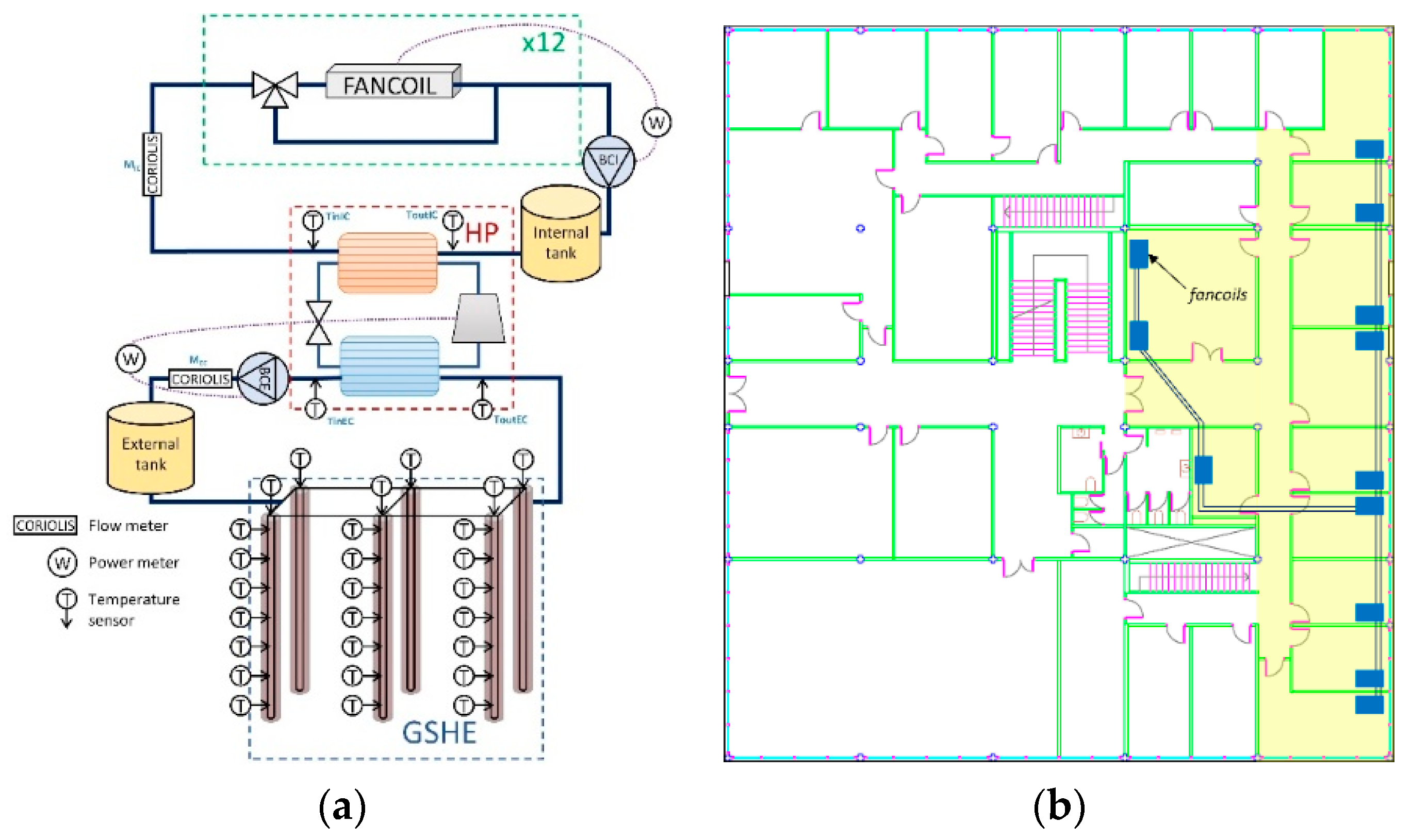
Figure 1a shows the schematic diagram of the installation. The system mainly consists of a water-to-water reversible heat pump which is coupled to the building through an internal hydraulic circuit and is coupled to the ground through an external hydraulic circuit. The different components of the system can be distinguished in Figure 1a: the heat pump (HP); the external circuit (EC) consisting of an external circulation pump (ECP), an external storage tank of 371 liters (which ensures a substantially constant temperature at the inlet of the ground source heat exchanger (GSHE) according to one of the purposes of the GeoCool project where the influence of the grout in the heat exchanger efficiency was analyzed), and the GSHE; and finally, the internal circuit (IC) consisting of an internal circulation pump (ICP), a buffer tank of 160 liters, and twelve fancoil units in the building whose distribution can be observed in Figure 1b.

The air-conditioned area comprises approximately 250 m², and, as can be observed in Figure 1b, includes nine offices located in the east façade of the building, a computer lab, and a coffee room. The heating/cooling distribution system in the building consists of a series of 12 parallel connected fancoil units. There is one fancoil unit per office, except for the computer lab where two fancoils are installed. The corridor is not air-conditioned. Each fancoil can be individually regulated by means of a thermostat and comfort temperature and fan speed can be selected by the user. A three way valve, which is controlled by the thermostat of the room, regulates the control for each fancoil allowing the heating/cooling water to be modulated through the fancoil in such a way that, when there is no need to keep on heating or cooling the room, the water flow rate is by-passed in the fancoil. The overall system operation is controlled by a timer which is programmed to operate between 7:00 a.m. and 9:00 p.m., five days per week, as the system is switched off during the weekends.

The heat pump that was installed in the framework of the GeoCool project consists of a water-to-water reversible heat pump, single-stage ON/OFF controlled working with propane, with a nominal heating capacity of 17 kW (35 °C water return temperature from the building loop/17 °C water return temperature from the ground loop), and 14.7 kW (14 °C water return temperature from the building loop/25 °C water return temperature from the ground loop) of nominal cooling capacity.

It should be noted that, in May 2011, in the framework of another FP7 European project called Ground-Med [31], the former heat pump was replaced with a new one consisting of two compressors of the same capacity in tandem, working with R410A. The new nominal heating and cooling capacities are 18 kW (35 °C water return temperature from the building loop/17 °C water return temperature from the ground loop) and 15.4 kW (14 °C water return temperature from the building loop/25 °C water return temperature from the ground loop), respectively. Another important change in the system was the removal of the external storage tank, as it was not necessary for the Ground-Med project purposes, and it was creating an extra pressure loss with the consequent increase in the ECP power consumption. Another modification was the change in the position of the internal buffer tank that was placed on the supply line to be able to control the supply temperature to the building and improve this way the user comfort.

The GSHE itself consists of six vertical boreholes arranged in a rectangular grid (2 × 3) with a 3 m separation between boreholes. Each borehole has a depth of 50 m and contains a single polyethylene U tube of 25.4 mm internal diameter and 32 mm of external diameter, with a 70 mm separation between the upward and downward tubes. The boreholes are backfilled with sand and, to avoid intrusion of pollutants in the aquifers, all of them are finished with a bentonite layer at the top. The values of the ground thermal properties (conductivity of 1.43 W/mK and volumetric heat capacity of 2.25 MJ/m³K) were obtained by means of a laboratory analysis performed on dry soil samples [32]. However, it should be pointed out that, as the phreatic level at UPV is 3.5 m, higher conductivity and volumetric heat capacity values are expected, as the surrounding soil might be saturated.

The operation of the heat pump is governed by an electronic controller which, depending on the temperature of the return water from the internal circuit (fancoils), switches on or off the compressor of the heat pump. The default values for the water return temperatures at the internal circuit can vary between 37 °C and 43 °C for heating mode and 12 °C and 15 °C for cooling mode. The ECP is governed by the controller of the heat pump, which activates the external circulation pump sixty seconds before activating the compressor and turns it off sixty seconds after the compressor. To vary the flow of water at the internal and external circuit, the circulation pumps’ speed is controlled by means of two frequency inverters, one for each circulation pump. The system is fully monitored by a sensor network, and the data have been collected by a data acquisition unit since February 2005. The experimental data have been deeply analyzed in [32,33].

Figure 1a shows the location of temperature sensors and flow meters on the hydraulic circuits, as well as the power meters. Values for the water temperature at the inlet and outlet of the heat exchangers existing in the heat pump are measured by means of four-wire PT100 with accuracy ±0.1 K. The water flow rate is measured at both the internal and external hydraulic circuits by means of two Coriolis flow meters with accuracy <0.1%. To measure the power consumption, two multifunctional power meters with accuracy ±0.5% of the nominal value are used, one for each circuit. The power meter of the internal circuit measures the power consumption of the fancoil units and the internal circulation pump; and the power meter for the external circuit measures the compressor and the external circulation pump power consumption. Additionally, the temperature and relative humidity in the offices is measured as well.

The installation that will be modeled and experimentally validated in this paper corresponds to the GeoCool installation. The experimental data considered for the model validation correspond to the year 2008. It should be noted that, in the results presented in this paper, the frequency for each circulation pump kept constant at 50 Hz in all the experimental measurements is considered. Consequently, the mass flow rate measured by both Coriolis flow meters (one for each hydraulic loop) was constant and equal to 3000 kg/h for the ICP and 2700 kg/h for the ECP approximately. As there are 12 fancoils connected in parallel, the water flow rate per each fan coil will be approximately 250 kg/h in the case that the fancoil is working. In case that the water is by-passed, the bypass has been designed to have the same pressure drop as the coil, so the total pressure losses in the internal circuit will keep constant and so will do the total flow rate.

The TRNSYS model was developed in such a way that the system design modifications that took place in the framework of the Ground-Med project during year 2011 can be easily implemented in the model, making it a useful tool to assist in the design and the development of energy optimization strategies in the system.

2.1. Typical Daily Performance

The control algorithm existing at the GSHP installation produces a very specific behavior of the different parameters of the system. More concretely, the influence of this control algorithm can be observed in the instantaneous response and the short-term behavior of the water temperatures at different points of the hydraulic loops.

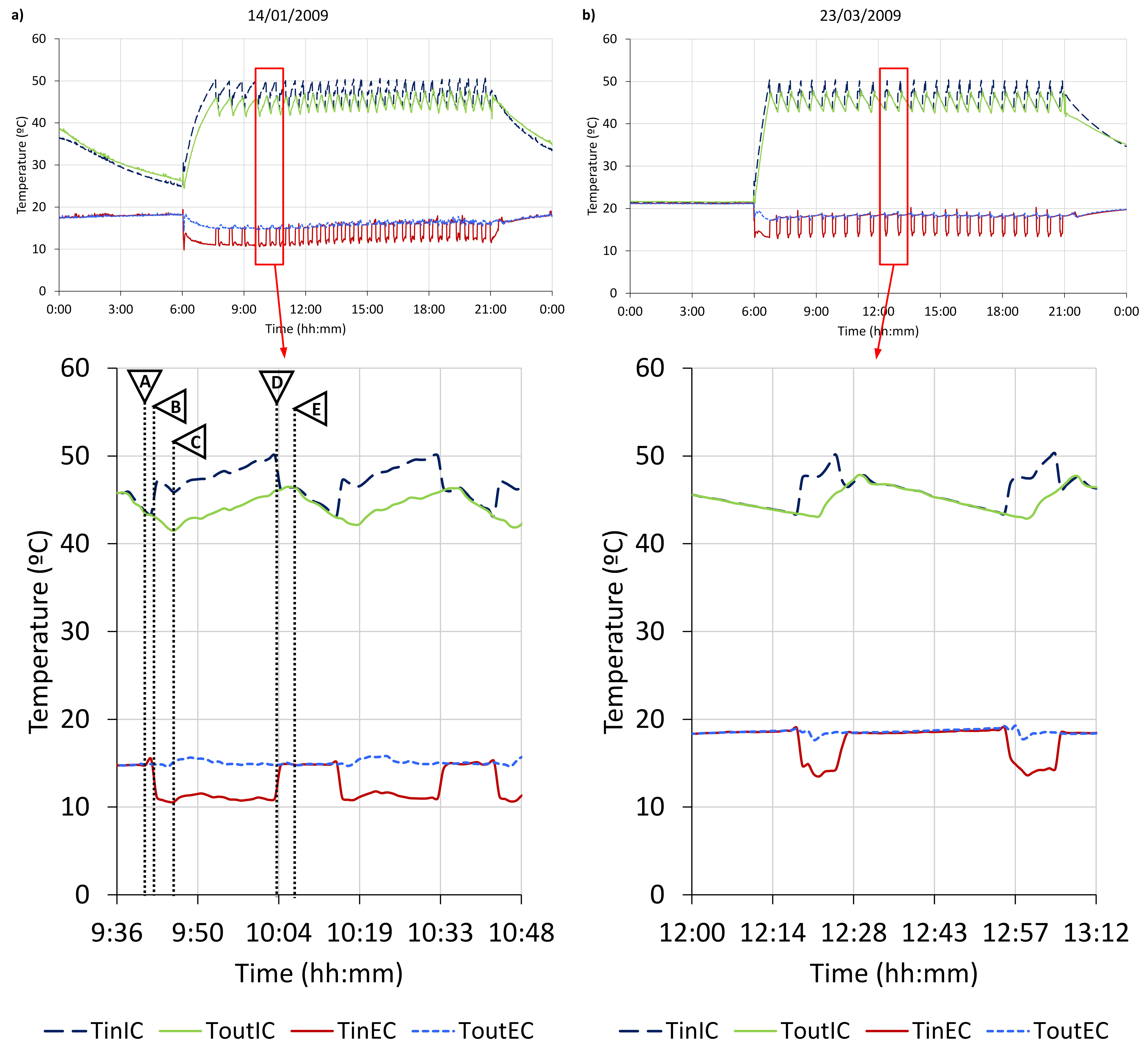
Figure 2 shows an example of the evolution of the water temperatures during two typical heating days, with different thermal load conditions. Figure 2a corresponds to a high load day and Figure 2b corresponds to a low load day. The main difference between both days is the duration of the ON and OFF periods of the heat pump. For higher load days, the period of time when the HP is switched on is higher than that of the lower load days. On the other hand, the internal circuit water temperatures vary between the same maximum and minimum values, depending on the temperature setting and deadband established in the control board of the system for each day. However, the external circuit water temperatures mostly depend on the ground temperature response. Therefore, the evolution of the water temperatures at the external circuit will reflect that of the ground temperature, which varies depending on the thermal load extracted in heating mode and injected in the case of cooling mode.

Looking at the instantaneous response of the temperatures, it is possible to identify the characteristic evolution corresponding to the ON/OFF cycling of the compressor and the ECP. Figure 2 also shows an augmented section of the daily evolution of the temperatures. To simplify the study of the cycles, several strategic points of the temperature evolution have been identified and labeled (A–E).

Looking at Figure 2, it is possible to detect, for the internal circuit temperatures evolution, a delay corresponding to the time that the water takes to circulate through the pipes. Thus, when the HP switches on (at point B), the temperature of the water returning from the IC still decreases for some more time, until the hotter water sent to the IC at point B has circulated through the fancoils and returns to the HP. Then, temperatures start increasing (point C). An analogous behavior can be observed when the HP is switched off. Since the ICP is continuously switched on, once the HP is switched off, the supply temperature equals the return temperature.

On the external circuit side, the behavior is slightly different, since the ECP pump cycles with the HP. Once the ECP switches on (at point A), and after some time (corresponding to the time that the water takes to circulate from the GSHE to the HP) it is possible to observe an increase in the return temperature, corresponding to the temperature of the water that was inside the GSHE during the OFF period. On the other hand, due to the delay between the switching of the HP and the ECP, the inlet temperature to the EC also equals the return temperature once the HP is switched off.

The short-term behavior of the water temperatures when the installation is working in cooling mode is analogous to that of the heating mode. However, in cooling mode, the temperatures of the EC correspond to the condenser in the HP and those of the IC correspond to the evaporator. Therefore, in cooling mode, the water temperatures of the EC will be higher than the IC ones.

3. TRNSYS Model

The main objective of the present work is to develop a complete model of the GSHP system located at UPV. To be able to correctly reproduce both the short-term and long-term behavior of the installation, a very detailed model is needed, which includes all the main components of the system.

For developing this model, TRNSYS [14] simulation software was chosen. TRNSYS interface allows combining individual models (types) for each component of the system and connecting them in a modular way to conform a complete model. Besides, it is also possible to modify the predefined types and create new ones, which provides a high versatility to the software. For these reasons, TRNSYS becomes one of the best options for developing a complete and very detailed system model.

To ensure a good accuracy of the results, a progressive incorporation strategy has been followed while developing the model. Thus, the first step consisted in creating the building model. Once the building was adjusted and validated with experimental measurements, the different components of the system were added to the model progressively, in three stages: fancoils, heat pump and IC components, and, finally, GSHE with the EC components. At each stage, the simulation results were compared to the experimental measurements to adjust and experimentally validate each single component of the installation. Using this strategy, it is possible to adjust each component individually. It also allows identifying the effect that each component has on the overall results of the simulation, thus simplifying the error detection and correction.

This section shows the different steps carried out during the model development and the main solutions adopted to reproduce the dynamic behavior of the system accurately. Section 4.1 shows the results of the model adjustment at each step and its experimental validation with the thermal load corresponding to the year 2008. Finally, Section 4.2 presents the validation of the complete model with the experimental data for the rest of the characteristic performance parameters.

3.1. Building

The building was the first component introduced in the model. All the constructive characteristics of the building, the offices and rooms have been considered to obtain a model of the air-conditioned area.

For this purpose, the TRNSYS building modeling complement, TRNBuild, has been used. In the TRNBuild application, the characteristics of the different spaces of the building were introduced, together with the information about the user’s behavior: lighting and usage schedules. Some parameters can still be adjusted to obtain a load profile of the building that corresponds to the experimental measurements: ventilation, infiltration, and temperature settings.

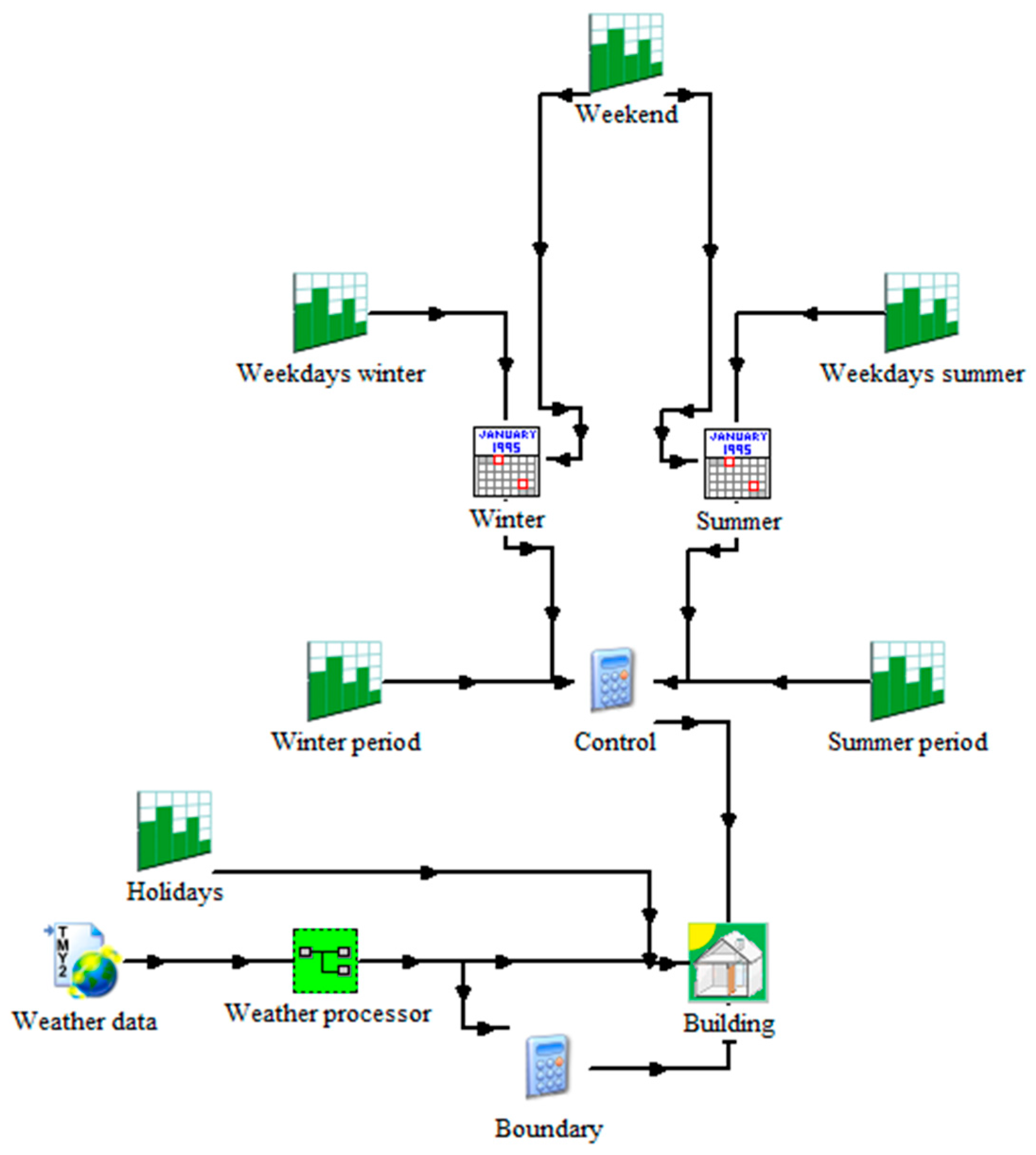
The building model developed with TRNBuild is included in a TRNSYS project. To be able to simulate the model, it is also necessary to include the information of weather conditions, which was taken from one of the TRNSYS meteorological libraries for the city of Valencia due to the lack of complete and detailed experimental information that was needed for the model On the other hand, the weather data from the TRNSYS libraries allow making the model more general as these libraries stand for an average of many representative years and not a specific one. Besides, it is also necessary to implement the basic control parameters of the installation: the schedules of operation of the installation for each day and the operation mode along the year.

The resulting TRNSYS model is presented in Figure 3.

3.2. Fancoils

Once the building is correctly modeled, it is possible to include the fancoils in the model. Each fancoil in the installation will be modeled individually and coupled to the corresponding room in the building. Moreover, since the behavior of the fancoils depends on the working mode, the model will be different for the fancoils in heating mode than in cooling mode.

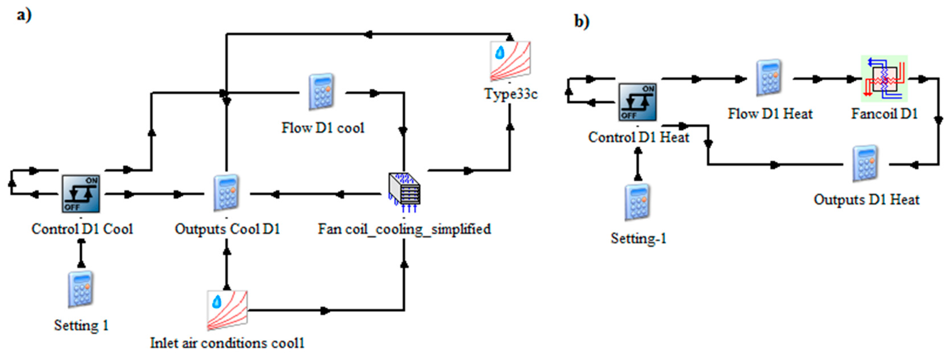
Figure 4 shows the two options used for modeling the fancoils. On the cooling mode model (Figure 4a), the fancoil is represented by the TRNSYS type 52, including the heat exchange and dehumidification functions. On the other hand, for the heating mode model (Figure 4b), the TRNSYS type 5 has been used, which only considers the sensible heat exchange between water and air in the fancoil.

The control of the fancoils has been implemented with the TRNSYS type 2, which models a differential ON/OFF controller. With this type, the reference temperature is compared to an upper and a lower bound. When the temperature increases above the upper bound, the control signal switches to 1. Then, when the temperature decreases below the lower bound, the control signal switches to 0. This control signal can be used directly for governing the fancoil switching in cooling mode, but it has to be inverted for the fancoil control in heating mode.

3.3. Heat Pump and Internal Circuit

The next step in the construction of the model of the system consists of including the heat pump. This involves including all the components existing between the fancoils and the heat pump: the internal circuit components. Therefore, in this step, the ICP, the internal storage tank and the distribution pipes will also be included in the model. The dimensions and geometrical characteristics of each of these components were checked in the real installation, and they were introduced in the model.

All these components are collected in a TRNSYS macro, with the scheme shown in Figure 5. For the ICP, the power consumption will be represented by an experimental correlation, depending on the water mass flow rate, which will be an input for the model, taken from the experimental data. The internal tank has been duplicated in the model to allow the user to choose if the tank is located at the supply (Ground-Med configuration) or at the return pipe (GeoCool configuration).

The model of the heat pump is based on the experimental correlations presented in [25]. To implement those correlations, a new TRNSYS type has been specifically developed for this application. The type includes, as a parameter, a scale factor that allows changing the size of the heat pump to analyze its impact on the system energy performance and/or to adapt it to other system configurations. The inputs of this type are the inlet mass flow rate and inlet temperature of the internal and external circuits. With these inputs and the scale factor, the heat provided to each circuit, as well as the power consumption of the heat pump, are calculated thanks to the correlations implemented in the type. The outlet temperature of each circuit is calculated from the inlet temperature and the heat injected/extracted to the fluid.

The same differential controller used in the fancoils model has been used also for the control of the heat pump, depending on the setting and deadband established for the reference temperature, which are taken as inputs for the model from the experimental data.

3.4. GSHE and External Circuit

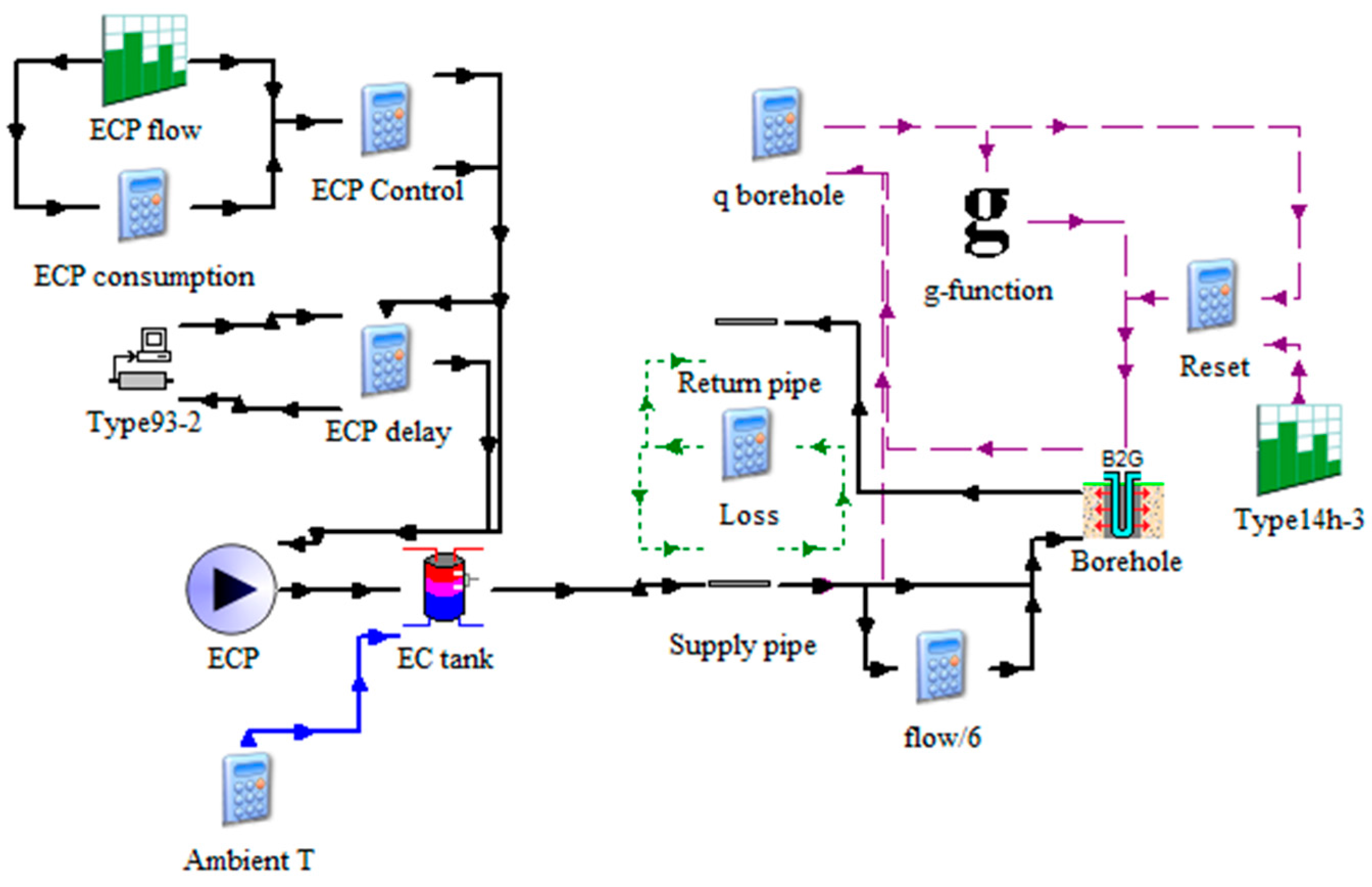
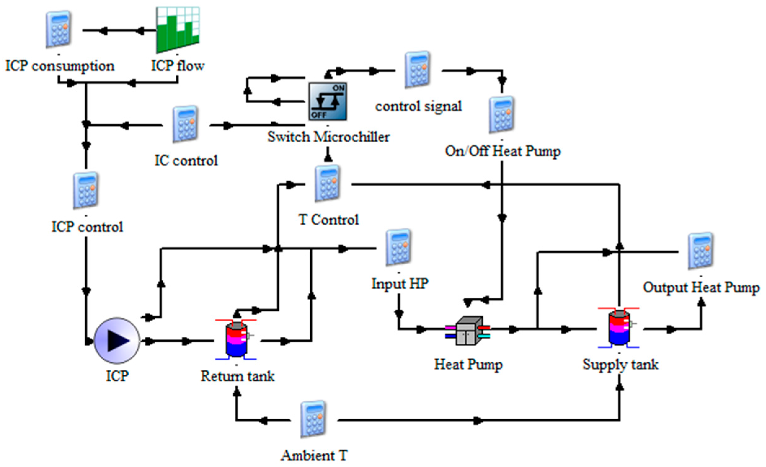
The last step corresponds to the GSHE model, and all the remaining components of the EC: ECP, external storage tank and external distribution pipes.

Again, for the ECP power consumption, an experimental correlation has been used, depending on the water mass flow rate. The electronic on/off control of this pump is taken from the controller of the heat pump, adding a delay of one minute using TRNSYS type 93.

For the GSHE, initially, type 557 was used, which implements the Duct Ground Heat Storage Model (DST) model [13]. However, this type only reproduces the steady-state response of the water temperatures of the GSHE, which produces significant differences on the shape of the temperature curves [34,35]. Therefore, it becomes necessary to use a dynamic model precise enough to model the instantaneous, short-term, and long-term responses of the GSHE, without excessively increasing the computational cost of the whole model. For this purpose, a new model was developed, called B2G (Borehole-to-Ground) model [27,28], that can predict the behavior of a borehole heat exchanger for a short period (10–15 h) with a great accuracy. This model can be combined with a long-term model to conform a complete GSHE model. The B2G model has been previously validated against experimental data from different installations [27,28], and compared with the DST model in the short-term prediction under two different conditions: a step-test (10 h of continuous heat injection) and the normal ON/OFF operation of a GSHP system, using experimental data from the installation located in Valencia. It was found that the DST was not able to predict the temperature delay in the outlet of the U-tube that occurs due to the water advection, while the B2G was able to reproduce it. Regarding the typical operation of the GSHP system, the DST does not reproduce correctly the response of the fluid inside the BHE, because it is based on a steady-state approach [35]. In the global model presented in this work, the B2G model will be coupled to the g-function model [8], which will be used only for the calculation of the long-term response of the GSHE. The coupling of B2G and g-function models has been presented and validated in [29].

The resulting scheme for the EC model is presented in Figure 6.

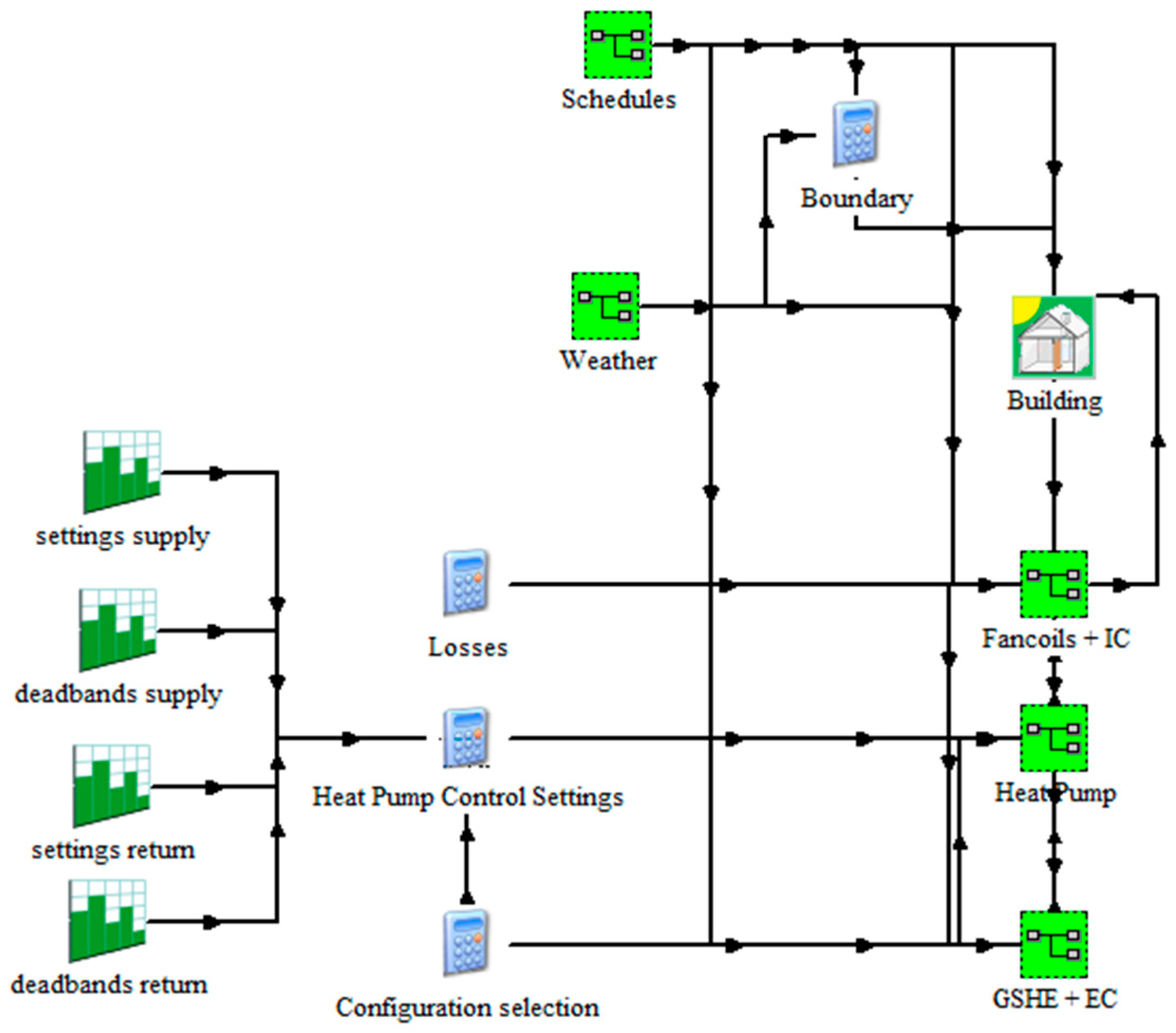
Figure 7 shows the final complete model in TRNSYS. As can be seen in Figure 7, the layout of the model is simplified using some TRNSYS macros to group the different types, which makes it more user friendly. Thus, all the schedules and timetable types (shown in Figure 3) are grouped inside a macro, and the same happens with the weather types. The macro corresponding to the fancoils contains all the fancoils modeled as shown in Figure 4. The heat pump macro contains all the components presented in Figure 5, and, finally, the external circuit macro contains the components from Figure 6. The corresponding types for establishing the settings and deadbands for the simulation are connected outside the macros, as can be observed in Figure 7.

At each of the steps considered in the model construction, an experimental validation was carried out to ensure the correct adjustment of each component. The different results obtained at each step as well as the ones corresponding to the final complete model are presented in Section 4.

4. Experimental Validation Results and Discussion

To simulate the complete system in TRNSYS, the different adjustment parameters for all the components were established taking into account the real values existing at the experimental installation. The control parameters (setting and deadband) were taken from the experimental measurements of the IC water temperatures. The simulation time step is one minute, corresponding to the sampling period of the DAQ system. The holidays were modeled by switching off some of the fancoils during these periods.

Section 4.1 presents the results of the adjustment at each step of the model construction. For the adjustment, the monthly average thermal load has been taken into account. It should be noted that the objective of the progressive incorporation strategy is not to obtain a perfectly accurate prediction at each step but to allow the individual adjustment of each component and, even more important than that, to study the way each of them affects the final results of the model. Once each component is correctly adjusted, the validation will be extended to the remaining parameters, in Section 4.2.

4.1. Progressive Incorporation

The experimental measurements allow the calculation of the thermal load of the heat pump. The actual building thermal load will be lower than the one measured at the heat pump, due to the thermal losses always present in these systems. Therefore, the first two steps in the model development (only considering the building and the fancoils) should produce thermal load values below the experimental ones.

Figure 8 shows the thermal load results corresponding to the first step of the model (series named Building in Figure 8), as described in Section 3.1, compared to the experimental calculation (series named Experimental in Figure 8). It should be noted that the values shown in Figure 8 stand for the average of the daily values of each month. Thus, they would stand for a typical daily load of each month. As can be observed in Figure 8, the experimental thermal load takes higher values in cooling season (from May to October) than in heating season. However, during August, there is an important reduction in the average thermal load, since most of the users are out of the office. This is the main reason why the total thermal load injected/extracted in the ground at the end of the year is balanced. The general evolution of the thermal load along the year is somewhat sinusoidal, with some exceptions for those months corresponding to vacation periods or unusual ambient conditions that affect the total thermal load. At this step, the simulated building thermal load is obtained directly from the building type (created with TRNBuild). As can be observed in Figure 8, the thermal load of the building correctly represents the behavior of the experimental one, always with a lower thermal load value as previously explained.

Figure 8 also presents the results corresponding to the second step (Section 3.2): including the fancoils (series named Fancoils in Figure 8). In this case, the thermal load also corresponds to the building thermal load, but it is obtained from the fancoils model. It should be noted that the temperature setting that was used to control the thermostat of the fancoils was calculated as the average between the surface of one of the walls of each room (in which the control sensor is located in reality) and the temperature of the air inside the room. Under these conditions, it is to be expected that the total modeled fancoils load is slightly higher than the building load calculated in TRNBuild. This is mainly because TRNBuild uses as the control temperature setting for heating and cooling that of the air located in a central point of the room. However, for the thermostats of the fancoils, the control temperature has been calculated taking into account not only the temperature of the air but also the surface temperature of one of the walls of each office, which presents a greater thermal inertia than the air. It is precisely this greater inertia that will cause an increase of the thermal load to be supplied by the fancoils. It can be observed in Figure 8 that, in months of greater thermal demand (January, February, July, August and December), the result obtained is similar in both cases. This is because the thermal capacity of the heating and cooling system considered in TRNbuild for calculating the thermal loads of the building is assumed to be infinite, while that of the fancoils is limited by the characteristics of the fancoil and by the selected operating speed of the fan. Thus, although at first the load of the fancoils should be greater than that of the building (due to the difference in the control temperature used), when the demand is high, the fancoils are not able to completely satisfy it, so the total thermal load supplied by the fancoils is less than what one would expect. On the other hand, for those periods in which the thermal demand is lower than the maximum thermal capacity of the fancoils (periods from March to April and from September to November), it is possible to observe an increase in the thermal load delivered by the fancoils with respect to that calculated only with the building in TRNbuild, as it is expected in these conditions of low building thermal load. Finally, it can be concluded that the results presented in Figure 8 for the fancoils thermal load still correctly reproduce the evolution of t the experimental thermal load.

Adding the heat pump to the model (Section 3.3) allows a fair comparison for the thermal load. In Figure 8 (series named HP in Figure 8), it can be observed that the thermal load measured at the simulated heat pump correctly predicts the experimental one, with very accurate values for most of the months.

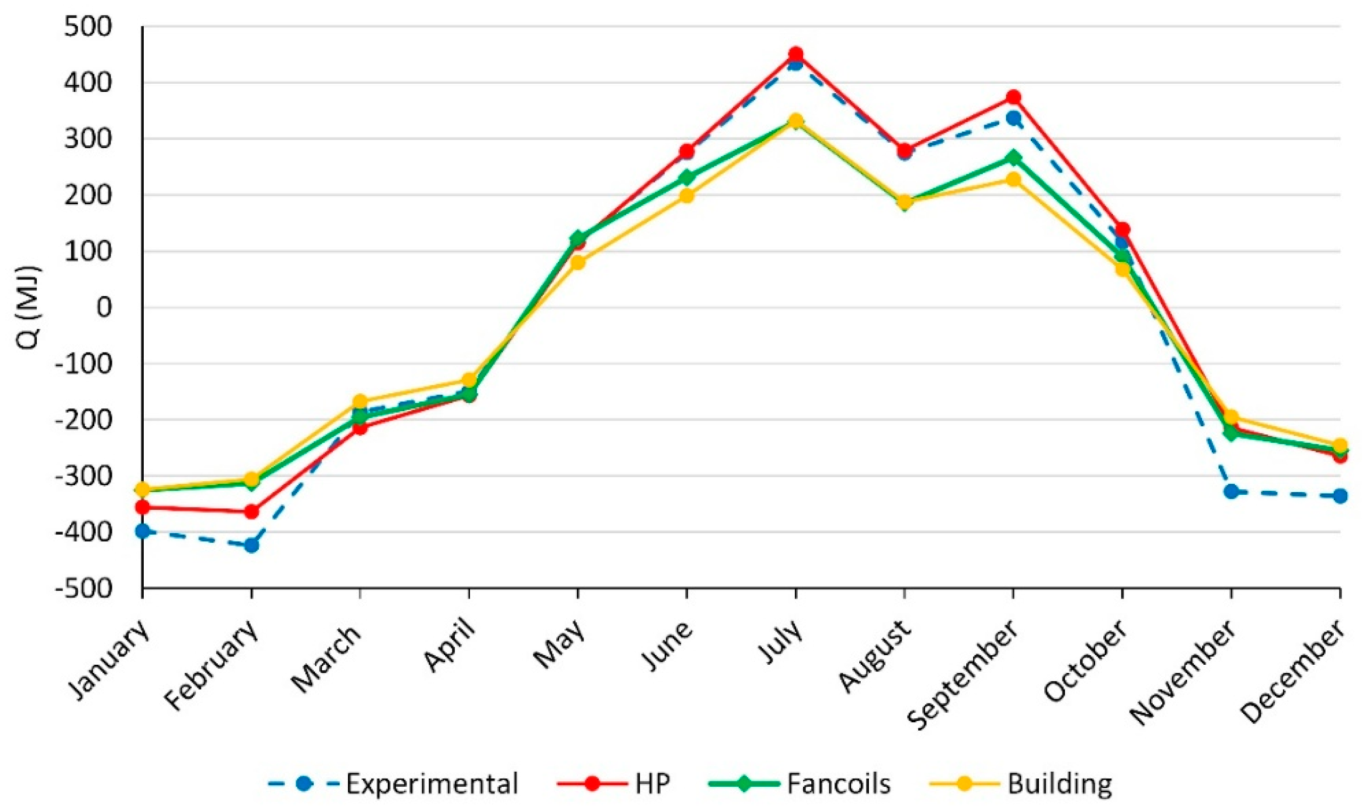
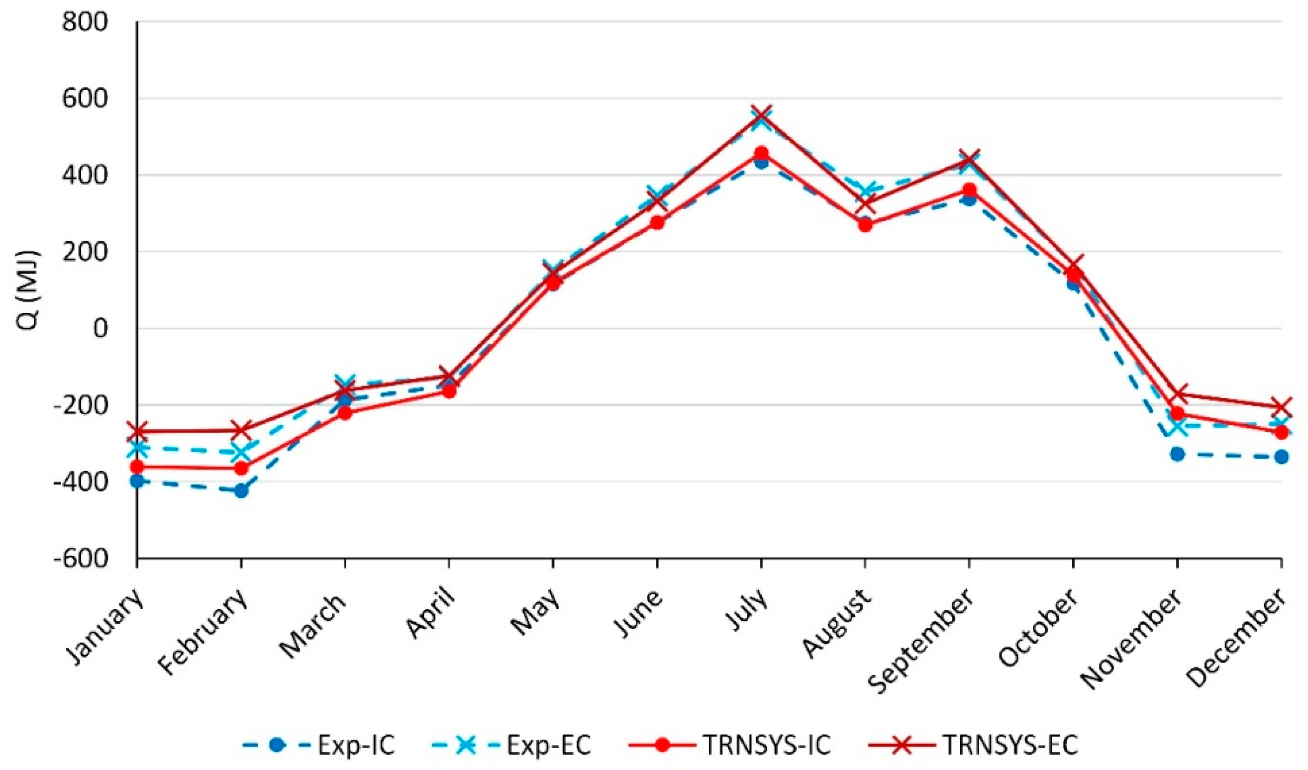
The final step consists of including the GSHE as described in Section 3.4, and both the internal circuit and external circuit thermal loads will be compared to the experimental ones. Figure 9 presents the corresponding results. The highest deviation from the experimental values corresponds to the thermal load of November. However, the experimental value of this month in year 2008 is greater (in module) than the typical one, mainly due to atypical ambient temperatures, cooler than usual. For the rest of the months, the complete model provides a very good prediction of the evolution and the trend of the thermal load along the year.

Since the model is aimed at representing a typical year of performance, the validation is considered satisfactory.

4.2. Global Model Results

The validation of the model will be extended taking into account the rest of the characteristic energy performance parameters of the installation.

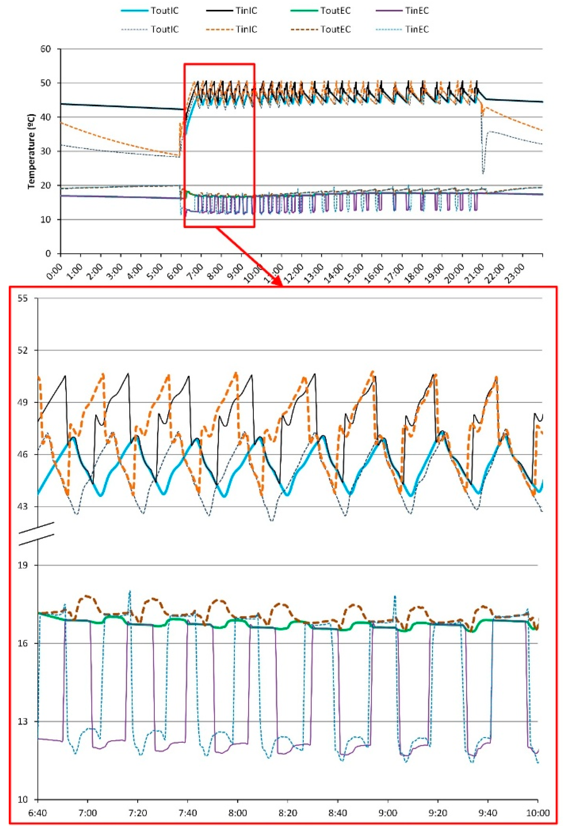
First, looking at the short-term evolution of the water temperatures, it is possible to validate the dynamic behavior of the model. Figure 10 shows a comparison between the simulated results on a typical day in heating mode and the experimental ones.

As can be observed in Figure 10, the evolution of the simulated water temperatures along the day correctly reproduces the experimental ones. Continuous lines correspond to simulated results and discontinuous lines correspond to the experimental measurements. Moreover, as shown in Figure 10, it is possible to observe the simulated evolution of the instantaneous response of the water temperatures caused by the ON/OFF control algorithm implementation. It can be concluded that the model is able to perfectly reproduce the same dynamic behavior observed in Section 2.1 for the evolution of the water temperatures during a heat pump cycle.

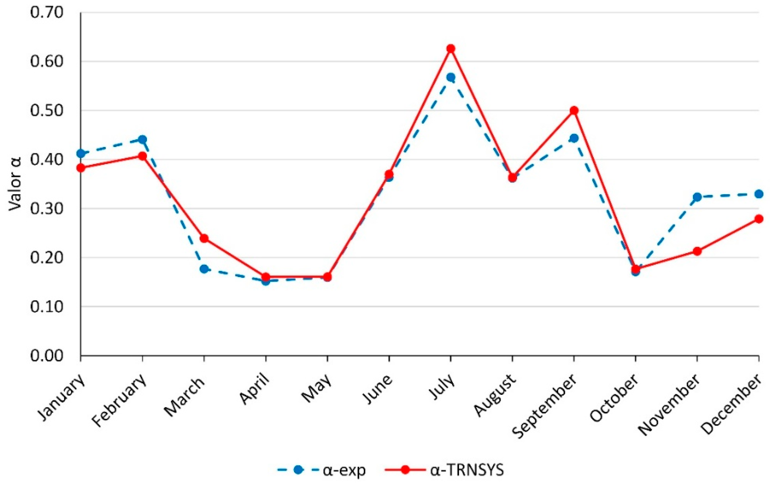
Looking at the long-term behavior of the system, one of the characteristic performance parameters to be studied is the average partial load ratio (α) for each month along the year, defined as the ratio between the thermal load and the maximum capacity of the heat pump. Therefore, the partial load ratio should present the same characteristics as the thermal load, provided that the heat pump capacity is correctly modeled. Looking at the partial load ratio evolution presented in Figure 11, it is possible to observe that this parameter perfectly reflects the evolution of the thermal load of the system. As can be seen in Figure 11, the evolution of the simulated partial load ratio is similar to the experimental one. The small deviations observed in Figure 11 reflect the ones observed in the thermal load (Figure 9); thus, it is concluded that the partial load ratio is correctly calculated by the model.

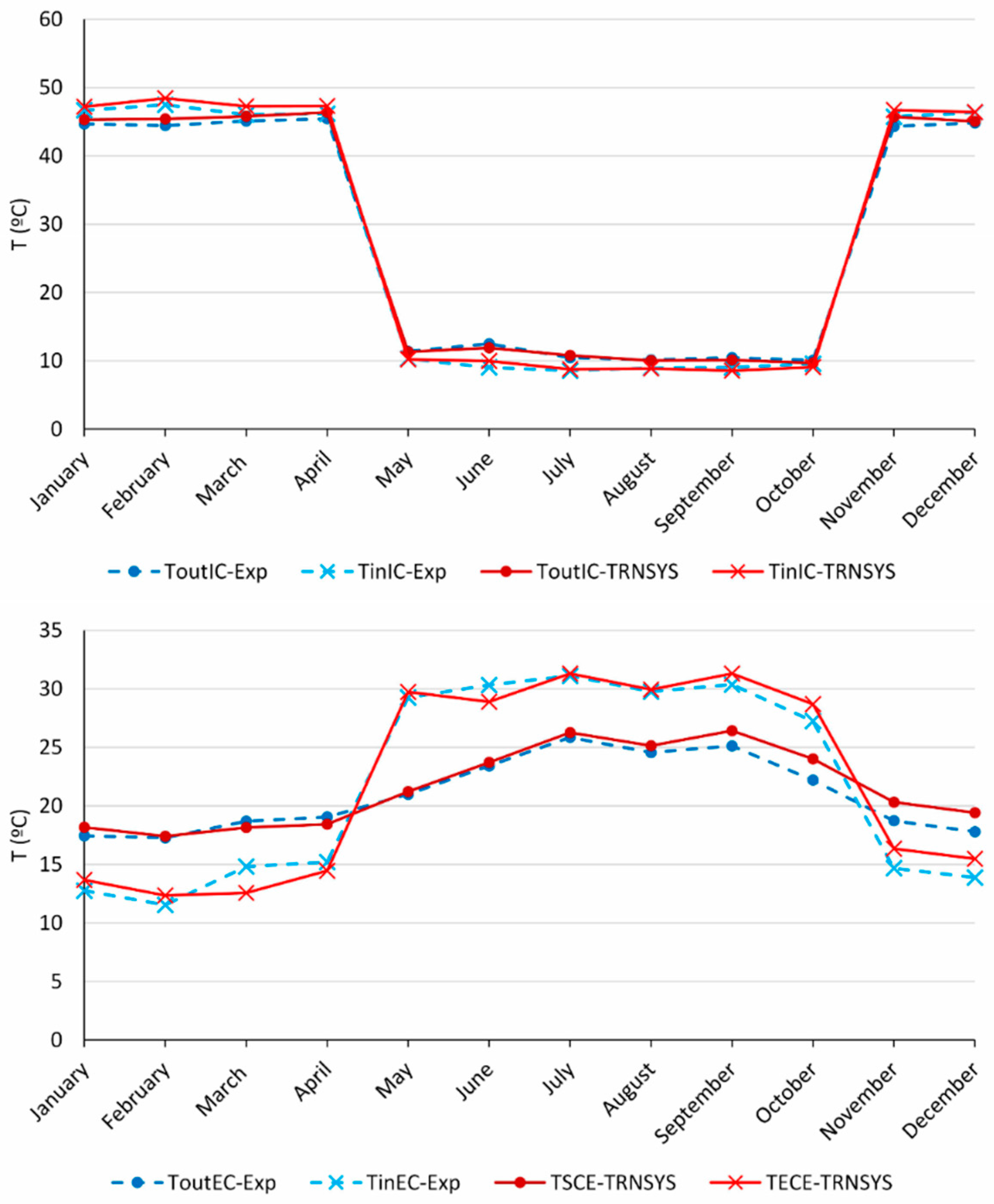
Besides analyzing the short-term evolution of the water temperatures, it is also interesting to observe the evolution of the average water temperatures along the year. Figure 12 shows the evolution of the average water temperatures at both sides of the heat pump. The IC temperatures mainly depend on the control setting values, so the adjustment will be correct as long as the setting in the simulation corresponds to the experimental one. On the other hand, the EC temperatures depend on the ground temperature and the thermal load. As can be observed in Figure 12, the simulated EC water temperatures present a good accuracy with respect to the experimental ones.

Finally, the last parameter to consider in the analysis is the energy efficiency of the GSHP system. This efficiency will be expressed as daily performance factors (DPFs), defined as presented in [33,34]. The DPF1 takes into account only the power consumption of the compressor. The remaining DPFs are obtained including in the calculation the other components of the installation: the ECP (DPF2), the ICP (DPF3), and the fancoils (DPF4). It should be noted that DPF4 includes the consumption of all the components in the system (HP, ICP, ECP and fancoils). The DPF prediction is one of the main features of the model. 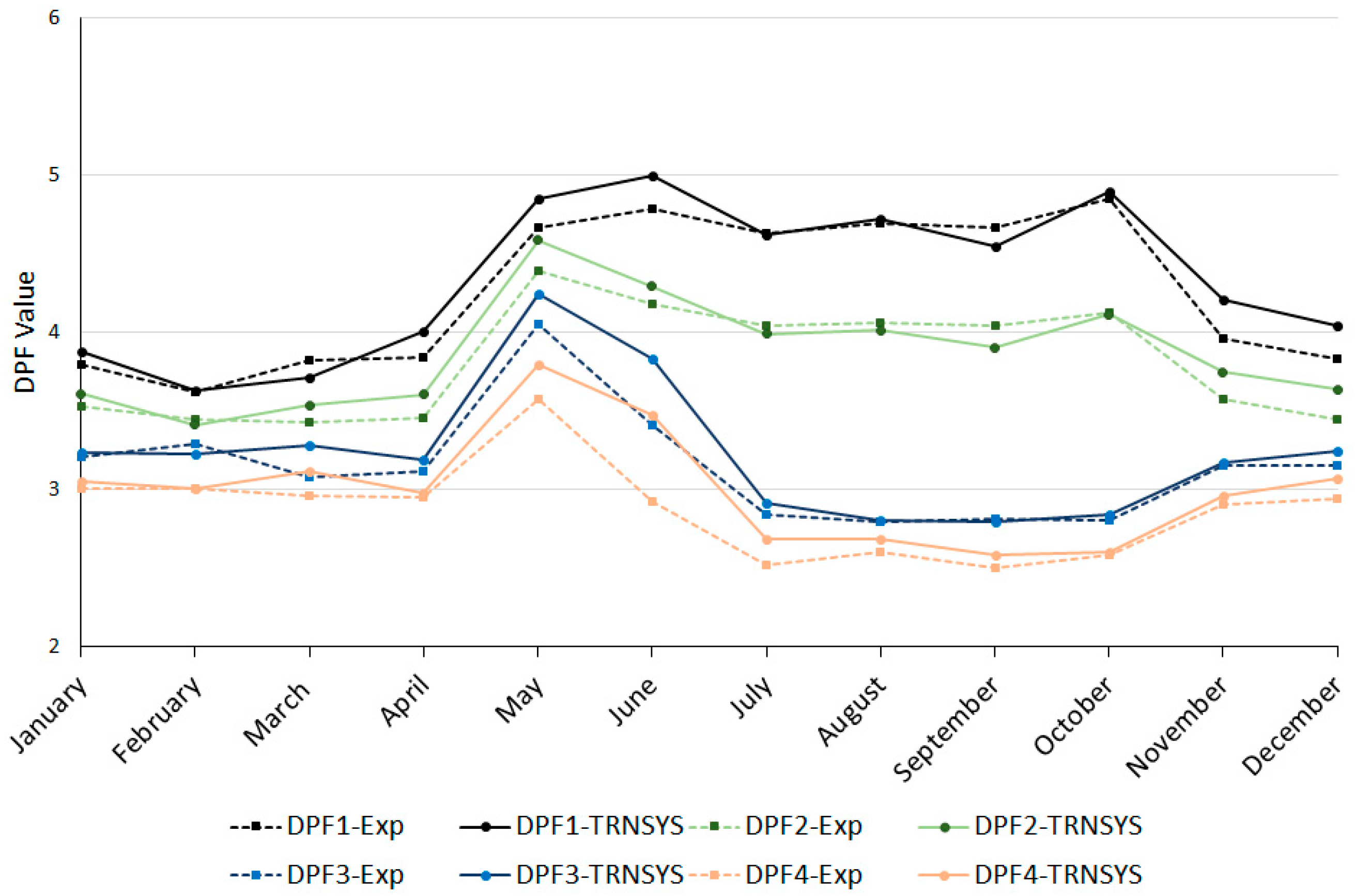Figure 13 shows a comparison between simulated and experimental DPFs. The experimental values correspond to the dashed lines; and the simulated ones, to the continuous lines. As can be observed in Figure 13, DPF1 and DPF2 take higher values in cooling mode (around 25% higher) than in heating mode, since the pressure drop that the compressor has to overcome is lower for this operating mode. When the ICP is included in the calculation, the heat that this component introduces into the IC water is also taken into account. This effect is positive in heating mode, but negative in cooling mode. Therefore, DPF3 and DPF4 have the seasonal variation compensated by the ICP heat load. On the other hand, as expected, including the power consumption of the different components has the overall effect of reducing the corresponding DPF value. Therefore, including the ECP results in a reduction of around 12% of the DPF2 with respect to the DPF1; the ICP produces an average decrease of around 13% of the DPF3 values; and the inclusion of the fancoils results in a 10% reduction of the DPF4 value.

As can be observed in Figure 13, the four DPFs calculated with the TRNSYS model follow the experimental results very accurately. The seasonal variation observed in the experimental results is reproduced on the simulated DPF1 and DPF2, and attenuated in DPF3 and DPF4. The influence of each component on the global efficiency is also correctly modeled, since the variation between the different DPFs in the simulation is the same as the experimental one.

In overall terms, the complete model developed has proven to be able to correctly reproduce the long-term and short-term behavior of the GSHP system located at UPV. The main performance parameters of the installation can be predicted by the model. Among them, the DPFs have a great importance, since they represent the energy efficiency of the system, thus, should be considered when improving the system’s performance. The model is able to correctly predict the evolution of the DPFs and the effect that the different components have over the global system’s efficiency. Therefore, this TRNSYS model will be a very useful tool for both the design and the energy optimization of the installation.

5. Applications of the Dynamic Tool Developed

The main utility of having an experimentally validated complete dynamic system model is that it fairly reproduces the reality acting as a virtual demonstration site. Therefore, it can be a tool to test and assess different modifications or operation strategies in the system without the need of implementing them in the real installation. Against this background, the model of the UPV system presented in this paper was used to assist in the development of optimization strategies and control algorithms before testing them experimentally. This was possible thanks to the fact that the system model is able to represent with a high accuracy the evolution of the DPFs, as presented in Section 4.2. Furthermore, it is possible to test the user comfort when the system is working under these optimization strategies, since it includes the coupling of the building to the rest of the system. With these control strategies, an improvement in the seasonal performance factor of the system (${\mathrm{SPF}}_{\mathrm{sys}}$) around 33% was achieved during the cooling season, always ensuring the user comfort [5].

Following the same methodology as the one presented in this paper, the dynamic system model was adapted to simulate the performance of a complete hybrid dual source heat pump system that was developed in the framework of the GEOT€CH European project [36]. In this case, the dual source heat pump is able to work using the air or the ground as a source/sink, depending on which one is the most favorable. The system includes, apart from the user and the ground loop, a Domestic Hot Water (DHW) loop with a storage tank and a free-cooling heat exchanger to use directly the fluid coming from the ground loop to provide cooling using only this heat exchanger instead of the heat pump. The model also includes a mid-season working mode, in which it assumes that the demand is met by natural ventilation and there is no need to use the heat pump or the free-cooling loop. This mid-season mode is enabled when the outside temperatures are close to the comfort temperatures in the building.

To adapt the TRNSYS model to the new hybrid dual source heat pump system, some minor modifications were carried out, thanks to the modularity of the model. First, the type of the heat pump was replaced for another heat pump model with the correlations corresponding to the hybrid heat pump. These correlations where obtained in a similar way than the previous ones.

The DHW loop that was included is similar to the internal circuit loop. In this case, a bigger water storage tank was implemented instead of the buffer tank and the building thermal loads were replaced with a DHW demand profile for an office building, using the same profile as the one considered in [37].

On the other hand, the free-cooling loop is modeled just by adding a simple model of a brazed plate heat exchanger. Finally, regarding the operation of the system, simple control strategies were implemented using differential controllers with hysteresis. Thus, the system selects the most favorable source depending on the temperature coming from the ground loop or the air temperature and it works in mid-season mode when the ambient temperature is close to the comfort one.

An analysis of the results calculated with the GEOT€CH system model applied to a demo-site that will be installed in Amsterdam, Netherlands, is presented in [37]. In this system, the ground would be used as a source 69% of the time in heating mode. During summer, the ground would also be the most used sink.

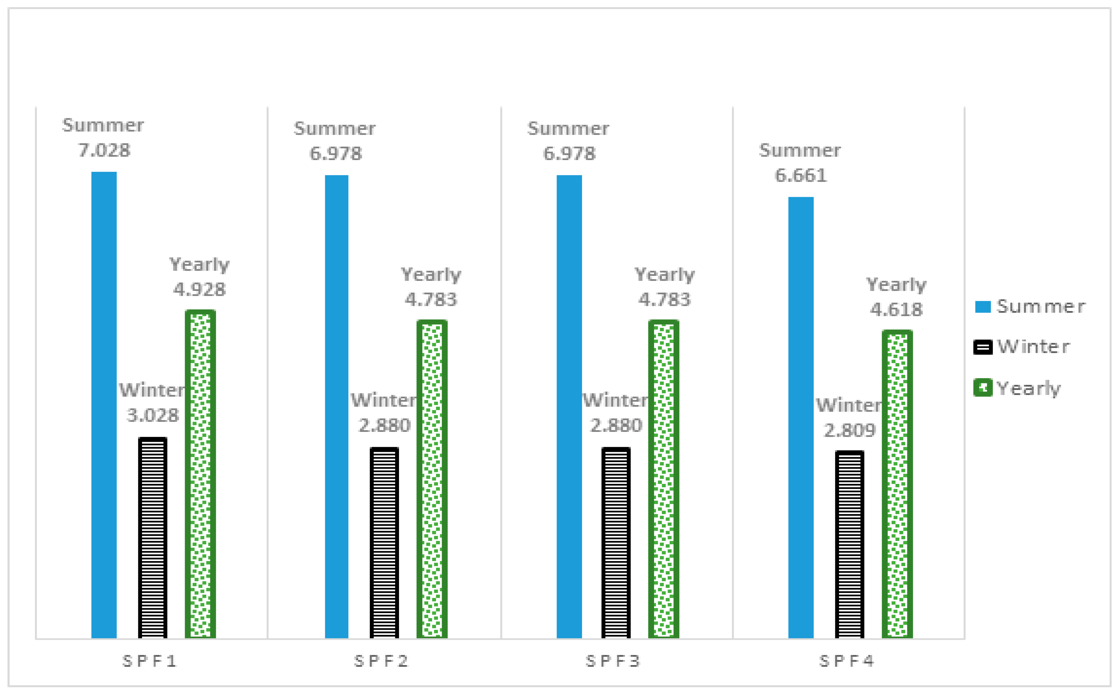
To see the applicability of this type of hybrid dual source heat pump in a different location, the system model has been adapted to the weather conditions in Valencia, Spain. It was agreed in the GEOT€CH project that the efficiency of the system would be analyzed by means of the SPFs defined in the SEPEMO European project [38]. SPF1 (Equation (1)) considers the heat provided to the user and DHW and the heat pump consumption; SPF2 Equation (2)) also considers the source consumption (fan and ground circulation pump); SPF3 (Equation (3)) also considers the backup heater consumption; and SPF4 (Equation (4)) also considers the consumption of the user and DHW loop circulation pumps.

$$\mathrm{SPF}1=\frac{{\int }_0^t\left({\dot{Q}}_{\mathrm{USER}}+{\dot{Q}}_{\mathrm{DHW}}\right)·dt}{{\int }_0^t{\dot{(W}}_{\mathrm{HP}})·dt}$$

(1)

$$\mathrm{SPF}2=\frac{{\int }_0^t\left({\dot{Q}}_{\mathrm{USER}}+{\dot{Q}}_{\mathrm{DHW}}\right)·dt}{{\int }_0^t{\dot{(W}}_{\mathrm{HP}}+{\dot{W}}_{\mathrm{FAN}}+{\dot{W}}_{\mathrm{BHE}})·dt}$$

(2)

$$\mathrm{SPF}3=\frac{{\int }_0^t\left({\dot{Q}}_{\mathrm{USER}}+{\dot{Q}}_{\mathrm{DHW}}\right)·dt}{{\int }_0^t{\dot{(W}}_{\mathrm{HP}}+{\dot{W}}_{\mathrm{FAN}}+{\dot{W}}_{\mathrm{BHE}}+{\dot{W}}_{\mathrm{BACKUP}})·dt}.$$

(3)

$$\mathrm{SPF}4=\frac{{\int }_0^t\left({\dot{Q}}_{\mathrm{USER}}+{\dot{Q}}_{\mathrm{DHW}}\right)·dt}{{\int }_0^t{\dot{(W}}_{\mathrm{HP}}+{\dot{W}}_{\mathrm{FAN}}+{\dot{W}}_{\mathrm{BHE}}+{\dot{W}}_{\mathrm{BACKUP}}+{\dot{W}}_{\mathrm{USER}}+{\dot{W}}_{\mathrm{DHW}})·dt}.$$

(4)

The SPFs obtained for the winter and summer season, as well as the yearly overall SPF are shown in Figure 14. It can be seen that the SPF obtained during the summer season is quite high (>6.5), which happens mainly due to the use of the free-cooling heat exchanger and the natural ventilation (mid-season mode). During the winter, the obtained SPF is lower (around 3). Finally, the yearly SPF has values between 4.6, for SPF4, and 4.9, for SPF1. A conclusion that can be extracted from this study is that there is a need to optimize the system operation during heating mode as it means around a 30% reduction in the yearly SPF4 compared to cooling mode. For this purpose, the dynamic system model could serve as an optimization tool for this system.

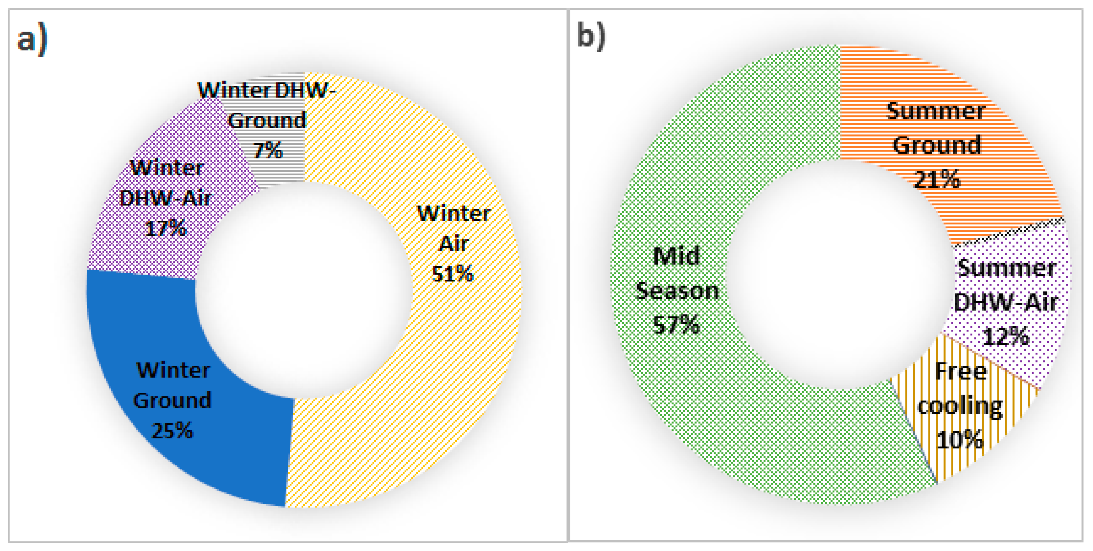
Figure 15 shows the mode in which the system is operating during the year. During the heating season, the air is the most used source because of the mild weather existing in Valencia during the winter. On the other hand, during the cooling season, the ground is the most used sink, although the air is the one used for DHW production, because the air is at a higher temperature than the ground. However, the system is working mostly in mid-season mode (only natural ventilation is needed) to meet the cooling demand.

Thus, it can be concluded that the use of this type of system would be convenient for a Mediterranean location such as Valencia, as it would lead to a reduction in the size of the ground source heat exchanger, and it would mean a higher yearly seasonal performance factor.

6. Conclusions

A complete model of a real GSHP system has been developed and presented in this paper. The model, developed in TRNSYS, is complete and detailed, including each of the installation components, modeled individually as well as their interaction in the system. For the development of the model, a progressive incorporation strategy was followed starting from the building and ending with the ground loop. The resulting model has proven to accurately simulate the performance of the system, in both the short-term and the long-term. Therefore, it constitutes a dynamic tool that can act as a virtual demonstration site. In this context, it will be possible to use the model to predict the effect that different modifications, either in the design or in the operation strategies, will have both in the dynamic and steady-state performance of the system. Besides, the model could be easily adapted to other GSHP systems by modifying the necessary components in TRNSYS or simply varying the adjusting parameters. As a practical case, the model was adapted to reproduce a complete hybrid dual source heat pump system to test its feasibility in the city of Valencia. It is concluded that the hybrid system is a good option for this type of Mediterranean climates, as it would lead to a reduction in the size of the ground source heat exchanger needed, and it would mean a higher yearly seasonal performance factor. Thus, the dynamic system model developed becomes a key tool for design and energy optimization purposes of low enthalpy geothermal energy systems for heating, cooling and DHW production.