Investigation of the Thermodynamic Process of the Refrigerator Compressor Based on the m-θ Diagram


1
School of Energy and Power Engineering, Xi’an Jiaotong University, Xi’an 710049, China
2
Nanjing Engineering Institute of Aircraft Systems, Shuige Road 33, Nanjing 211106, China
*
Author to whom correspondence should be addressed.
Energies 2017, 10(10), 1517; https://doi.org/10.3390/en10101517
Submission received: 25 August 2017
/
Revised: 16 September 2017
/
Accepted: 25 September 2017
/
Published: 1 October 2017
(This article belongs to the Section I: Energy Fundamentals and Conversion)
Abstract
:The variation of refrigerant mass in the cylinder of refrigerator compressor has a great influence on the compressor’s thermodynamic process. In this paper, the m-θ diagram, which represents the variation of refrigerant mass in compressor cylinder (m) and the crank angle (θ), is proposed to investigate the thermodynamic process of the refrigerator compressor. Comparing with the traditional pressure-Volume (p-V) indicator diagram, the refrigerant’s backflow trigged by the delayed closure of valve can be clearly expressed in the m-θ diagram together with the mass flow rate. A typical m-θ diagram was obtained by experimental and theoretical investigations. To improve the thermodynamic model of the compressor, a 3D fluid-structure interaction (FSI) FEA model has been introduced to find out the effective flow area of the valves. Based on the m-θ diagram, the effect of rotating speed on the backflow through the valve, which depends on the movement of the valve, has been investigated. Specific to the compressor used in this study, the maximum backflow through the suction valve and discharge valve occur at 3500 r·min−1 and 5500 r·min−1, respectively.
1. Introduction
Lower energy consumption and eco-friendly domestic refrigerators are definitely the development direction for all researchers and engineers facing the common issue of reducing global warming. In fact, the electricity consumption of refrigerators is among the highest of all consumer household appliances, and it is highly dependent on the compressor efficiency.
The thermodynamic process of the compressor is a key indicator of the compressor’s energy efficiency. Several key factors govern the thermodynamic process of a refrigerator compressor, including pressure and temperature in the cylinder, the motion of the valve, etc. The understanding of the relationship between these key factors is essential to optimize and improve the efficiency of the compressor.
Ribas et al. [1] indicated that gas superheating in the suction line might account for 49% of the overall thermodynamic energy loss in the refrigerator compressors. Fabrício et al. [2] pointed out that thermodynamic losses are linked to the flow of refrigerant gas inside the compressor. In the suction process, the main losses are the superheating of refringent, flow losses in the suction muffler and through the suction valve, including backflow. The optimization of the suction and discharge valves in the plastic suction muffler has already led to considerably improved efficiency. Morriesen et al. [3] revealed that the thermodynamic parameters during one cycle were strongly linked to the valve motion, including displacement and velocity in the suction chamber.
Many numerical and experimental investigations on the thermodynamic process of a reciprocating compressor have been carried out recently in order to focus on improving the compressor efficiency, as described below.
Numerical tools are very helpful to understand the compressor’s thermodynamic process more economically and efficiently. The first thermodynamic model of the reciprocating compressor was developed by Costagliola [4]. Valve dynamics were considered in the model. This model was widely applied in many reciprocating compressor studies, and various improvements have been made. Sun et al. [5] improved the thermodynamic model by considering other factors, such as heat transfer, leakage, gas pulsation and valve motion. Stouffs et al. [6] proposed a method to obtain volumetric efficiency based on this model and presented the functional relationship between volumetric efficiency and discharge pressure, which was then verified by the experimental data. In order to calculate the volumetric efficiency of the compressor, Perez-Segarra et al. [7] studied the key factors that affect the volumetric efficiency, such as heat transfer and pressure drop, leakages, super-discharging, and supercharging. He argued that with the compression ratio increasing, the irreversibility caused by heat transfer and pressure drop exacerbated the volumetric efficiency. Farzaneh-Gord et al. [8] constructed a thermodynamic analysis for natural gas reciprocating compressors based on real and ideal gas models. Thiago Dutra et al. [9] developed a comprehensive simulation approach for hermetic reciprocating compressors including modeling of the electrical motor. Isacco Stiaccini et al. [10] developed a hybrid numerical model to simultaneously carry out the time-domain analysis of the compressor thermodynamic cycle and the frequency-domain acoustic analysis of the pipeline system. Liu et al. [11] has built a mathematical model coupled with compressor, actuator and hydraulic system.
As for experimental studies, Ma et al. [12] measured the volumetric and thermodynamic efficiencies of a CO2 compressor under various operating conditions and found that with the increase of the discharge pressure, the volumetric efficiency decreases while the total isentropic efficiency maintains a constant. Nagata et al. [13] measured the motion of the suction valve of a hermetic reciprocating compressor for a domestic refrigerator with a strain gauge. Real et al. [14] measured the valve motion in a small hermetic compressor using a fiber optic displacement sensor.
In these cited literature above, the thermodynamic process are often analyzed by a traditional p-V diagram, which shows the pressure variation as a function of the piston position. The indicated work is calculated by the integral of p and V in one cycle [6]. It is worth noting that an experimental p-V indicated diagram of a trans-critical CO2 reciprocating compressor was obtained by Ma et al. [4], and the flow losses related to the discharge and suction valves based on the p-V diagram were also presented.
In this paper, the m-θ diagram, which stands for the variation of refrigerant mass in cylinder (m) and the crank angle (θ), is obtained using the thermodynamic model of the compressor as a new tool to study the compressor efficiency. The thermodynamic model took into account the effective flow area for the valves, which has been obtained from flow through the valve using the Fluid Structure Interface model. This method is considered more reasonable compared to the conventional empirical flow coefficient. Furthermore, the influence from the rotating speed has also been identified based on the m-θ diagram.
2. Thermodynamic Model and m-θ Diagram
As shown in Figure 1, the thermodynamic model for compressor cylinder consists of three control volumes and mass transfer through the suction and discharge valve. The mass transfer is often coupled with the variation of control volume and valve motion. Based on this thermodynamic model, the m-θ diagram could be calculated.
2.1. The Governing Equation in Control Volume
The control volume includes the cylinder Vc, the suction chamber Vs, and discharge chamber Vd, which were a typical open thermodynamic system. The volume of the suction chamber and the exhaust chamber is constant. The working volume of the chamber varies following the function of crank angle as:
The energy conservation of the three control volumes is described as:
The mass conservation of the three control volumes is described as:
As the refrigerator compressor speed is higher, the leakage ml can be ignored.
The pressure variation in the control volume can be calculated by using the following equation:
In current numerical model, the working fluid is R600a, and material properties of this fluid are obtained from NIST REFPROP.
The variation of specific volume with rotation angle calculated by the equation as follow:
2.2. The Mass Flow Model through Valve
In the thermodynamic model, as shown in Figure 1, the flow through the valve was simplified as a nozzle, and the mass flow is then estimated as follows:
where β is the flow coefficient of the valve. The p1 is the inlet pressure of the nozzle model. The γ is the pressure ratio of the nozzle model. A is the valve clearance area and k is the adiabatic exponent. Flow coefficient β was defined in Equation (7) and obtained by FSI model and will be discussed in Section 2.3.
2.3. Flow Coefficient β
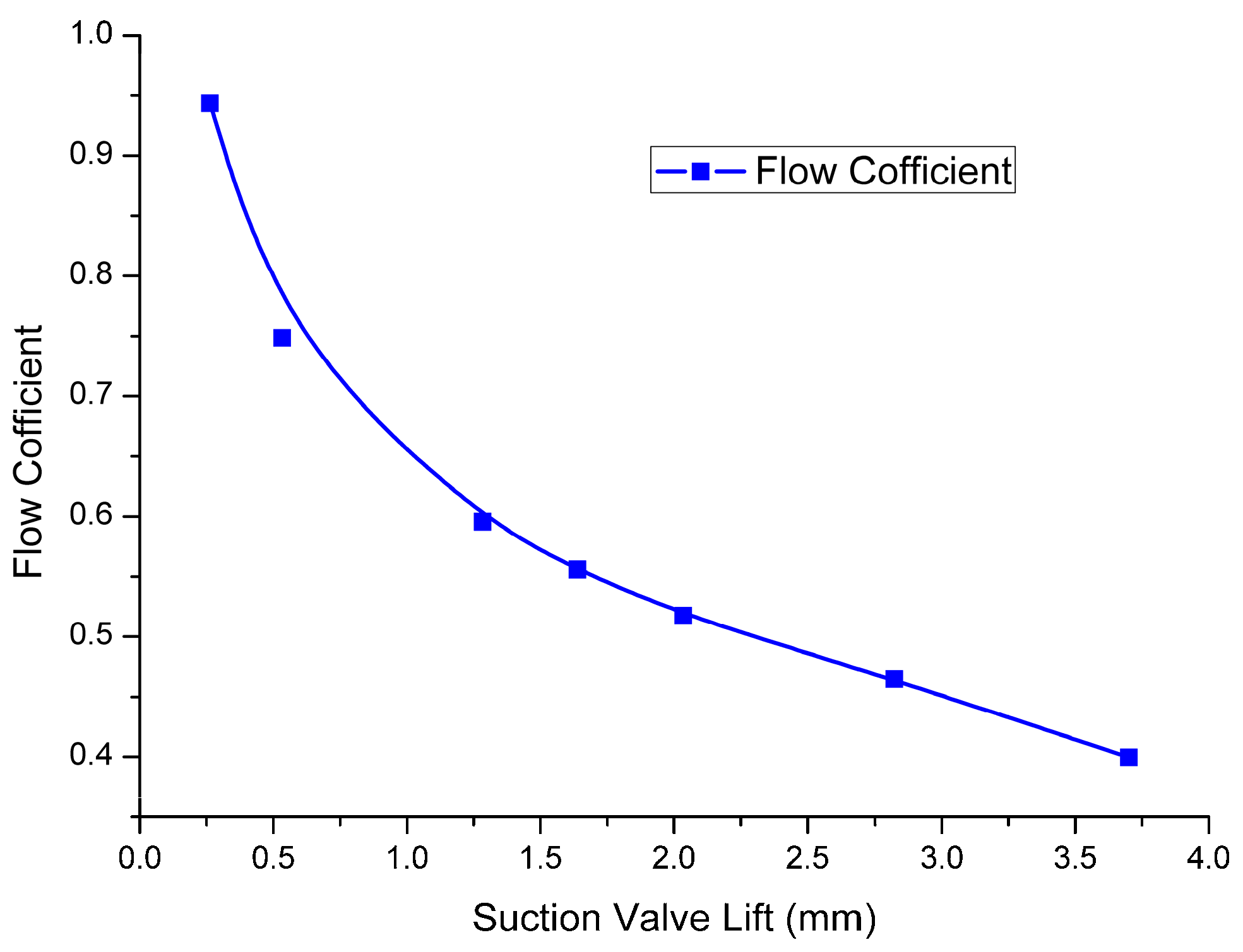
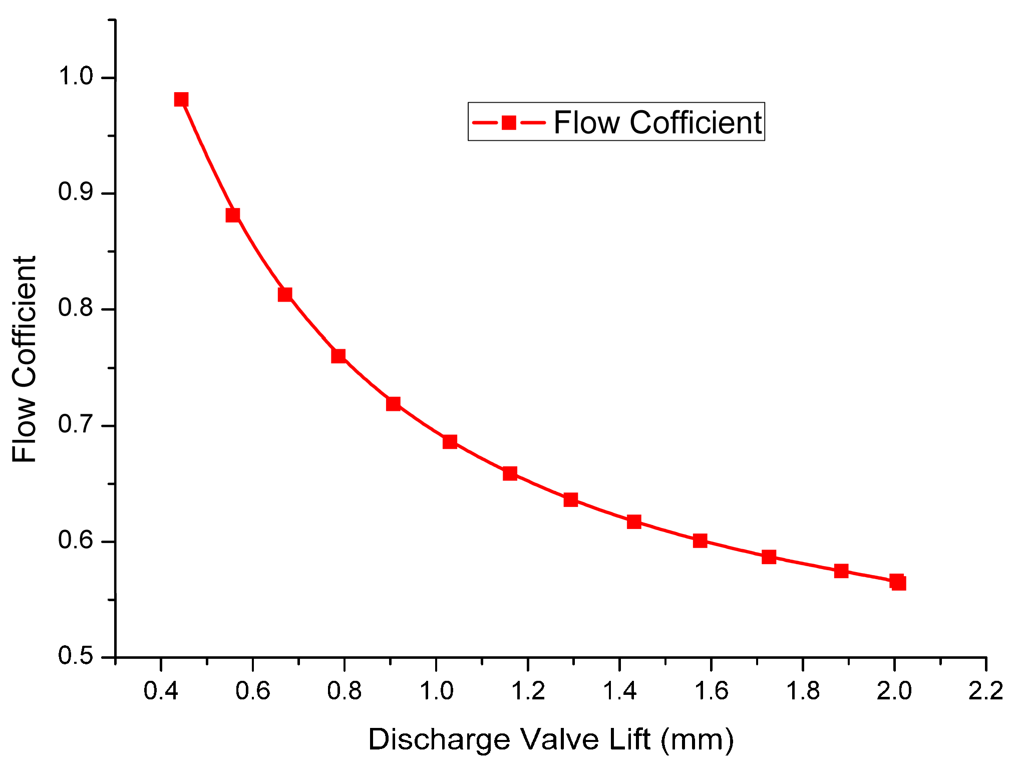
The flow coefficient β has a significant influence on the flow rate of the compressor since that the variation of refrigerant mass in the compressor cylinder is very dependent on the flow coefficient of the suction and discharge valve. The traditional method to obtain the flow coefficient of the valve is experiment blowing through the valve. Nowadays, with the development of CFD and FEA technology, the flow coefficient can be obtained with a numerical method [15].
The flow of refrigerant through valve and the valve motion are coupled with each other. The reed valve will experience bending deformation under refrigerant load. The deformed valve and its motion, in turn, affects the flow of refrigerant. This coupling ma the estimation much more complicated.
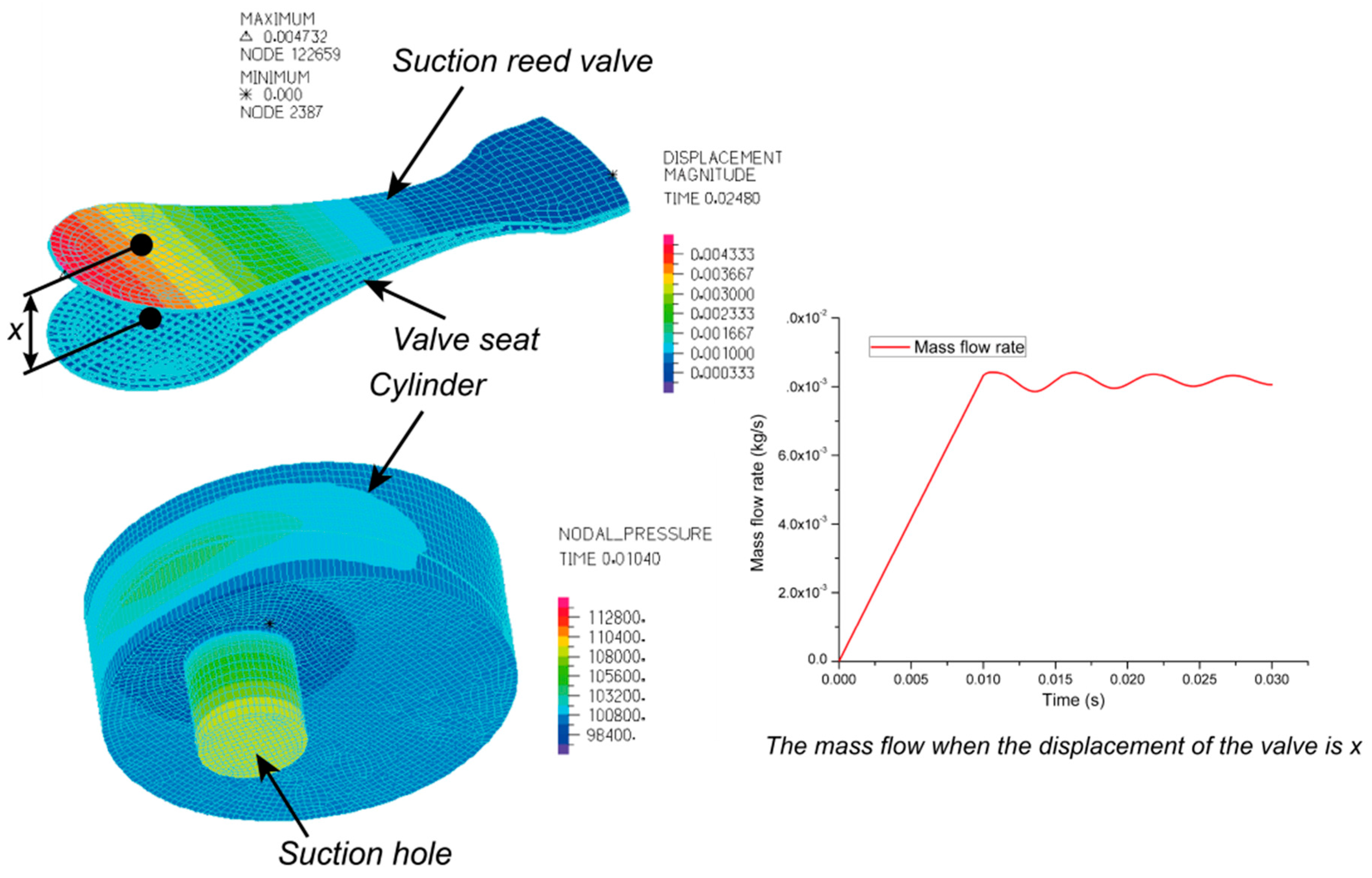
In this study, a transient FSI valve model was established to obtain the flow coefficient at various valve lifts. The FSI valve model of suction side is shown in Figure 2. The FSI model is divided into the fluid domain and corresponding solid domain.
To solve the FSI model, the fluid domain is analyzed based on the finite volume method, and the solid domain is analyzed based on the finite element method. Subsequently, the coupled solution of the two domains was implemented using the FSI solver. Governing Equations for the compressible flow including mass, momentum, and energy in the fluid domain and governing equations for the solid domain have been solved together for the FSI model using the commercial solver, ADINA version 9.0.6. The fluid domain was discredited using 8 node 3D element. The RNG k-ε model is employed to simulate the turbulent flow. The mesh size was 0.5 mm. The time step was 5 × 10⁻⁴.
The computer time is about 3 h based on 8-core Intel processor i7-4930K, with 3.40 GHz and 32.0 GB RAM.
Based on the numerical method discussed above and the nozzle model, the flow coefficient can be defined as the ratio of the numerical calculated mass flow rate to the ideal mass flow rate defined in Equation (6) from the isentropic relations, as follows:
where the is the calculated mass flow though the valve, which obtained by the numerical method.
2.4. The Valve Dynamics Model
In the thermodynamic model of the compressor, the reed valve was simplified as a spring-mass-damper system of single freedom. Assuming that the refrigerant flow on the valve plate is not biased and considering the gas force and the deformation force acting on the reed valve, the general equation of motion for a valve plate is then determined as follows [14]:
where K is the effective spring stiffness and M is the effective mass, which can be obtained by the finite element method. The frequency of valve flutter is typically close to the fundamental natural frequency of the valve. For an equivalent model of reed valve, the natural frequency in Hz is
Table 1 shows the natural frequency, the equivalent mass and the equivalent stiffness calculated by the FEM analysis and the experimental natural frequencies measured for the suction and discharge valves [14]. Comparing the natural frequency predicted by FEM analysis with that measured by the experiment, the FEM method for the natural frequency and the equivalent mass of reed valve meets the engineering requirements.
2.5. Solution Methods for the Thermodynamic Model
Taking control volumes as the object of study, the energy equation, the mass equation, the valve dynamics equation and the volume change of the cylinder can be regarded as a function of the rotation angle and are sorted into the following ordinary differential equations:
In Equation (10), Equation (10a) corresponds to Equation (4) for pressure variety in the cylinder, Equation (10b) corresponds to Equation (3) for the refrigerant mass variety in the cylinder, Equation (10c) and (10d) correspond to Equation (8) for the valve movement, and Equation (10e) corresponds to Equation (5) for the refrigerant density variety in the cylinder.
These differential Equations are solved by using the 4th order Runge-Kutta method. The convergence criterion is that the maximum pressure difference and temperature difference between the two iterations at the same crank angle location are less than the set tolerance. The flow chart for the thermodynamic model of refrigerator compressor is shown in the Figure 5.
2.6. The m-θ Diagram
Based on the thermodynamic model, the m-θ diagram was obtained, as shown in Figure 6. Compared with the traditional p-V diagram, the working process of the compressor in the m-θ diagram is divided into six phases, namely the backflow phase through discharge valve (1–2), expansion phase (2–3), suction phase (3–4), backflow phase through suction valve (4–5), compression phase (5–6), discharge phase (6–1). The analysis of the backflow phases could be used to characterize the influence of the compressor valve on the mass flow rate. The difference between mass in compression phase and mass in expansion phase is the mass delivered by the compressor during a working cycle.
3. Experimental Setup and Procedure
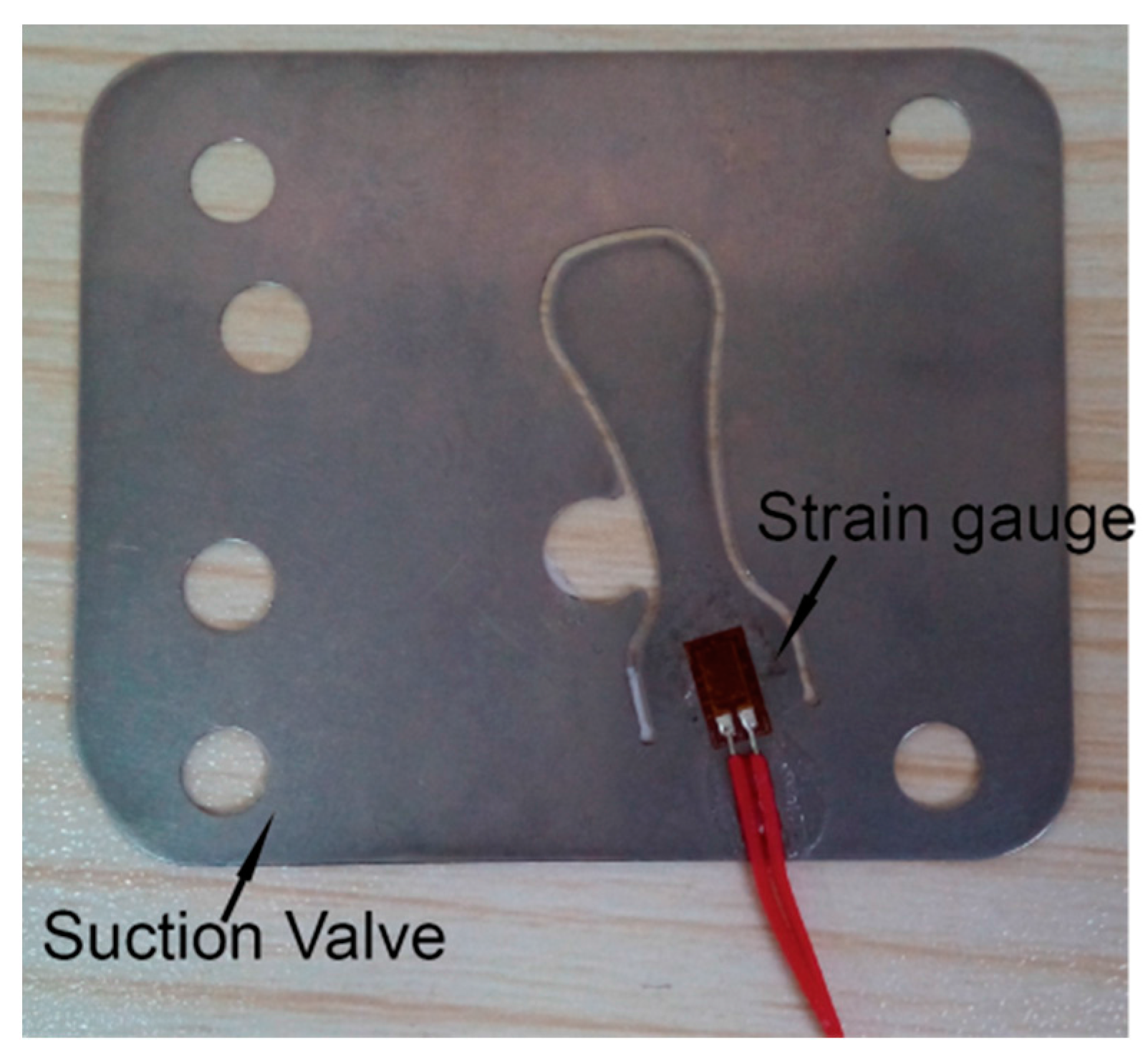
The experimental focus of this study is the pressure in the cylinder and the suction valve motion. In order to facilitate the installation of sensors, a refrigerator compressor (Qianjiang, WQ153Y) has been modified as shown in Figure 7 and the structural parameters of the compressor are listed in Table 2.
Recording the p-V diagram in the experimental study was delicate due to the small size of the refrigerator compressor. The high-precision pressure sensors (Kulite, XT-190(M)), with the sampling rate of 50 kHz and measurement accuracy of 0.1%, were used to measure the transient pressure history. The sensors were installed with careful consideration of the dimensions and the actual structure of the compressor. As shown in Figure 8, the sensor for recording the pressure in the cylinder was embedded in the valve seat to have the least influence on the flow structure.
Based on the operating parameters of the refrigerator compressor, the special strain gauge sensor (120 Ω) was selected [14] as shown in Figure 9, considering the seal under the transient high-pressure condition and the limited installation space. The simultaneous bridge module (NI 9237) was used to collect the strain signals from the quarter Bridge (NI 9944) with the strain gauge, whose measurement accuracy was 1.0%.
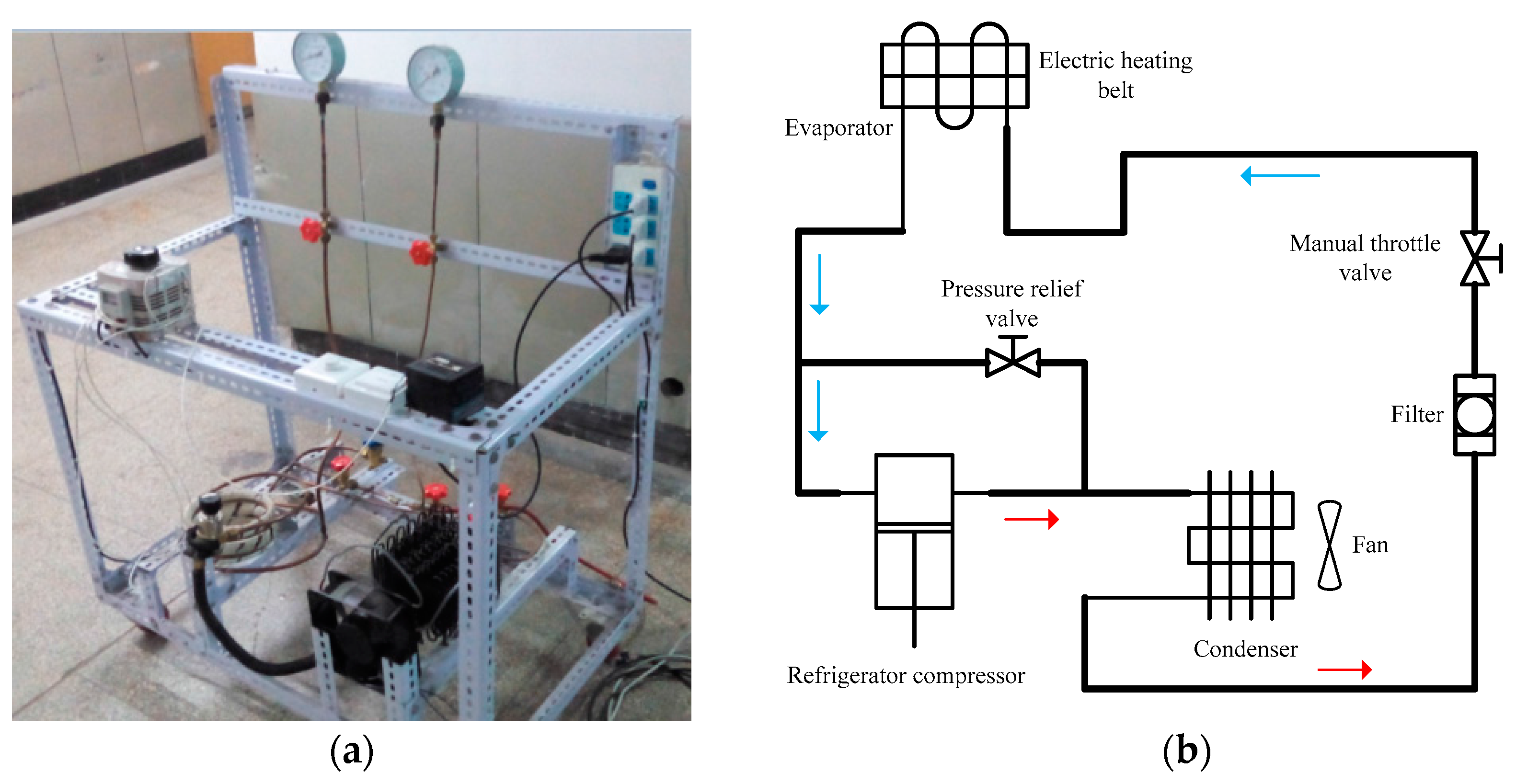
The refrigeration system used to establish the different operation conditions for the compressor in this study is shown Figure 10. The main refrigeration loop consisted of a compressor, a condenser, a manual throttling valve, an evaporator and other additional components as shown in Figure 10b. A heating belt was used to heat the evaporator representing the heating source while a balance valve was used to connect the evaporator and the condenser during the process for charging refrigerant. A variable frequency fan was used in the system to release the heat from the condenser.
The experimental procedure used for validation tests can be summarized as follows: The compressor was running for over 20 min in order to reach the constant working states of suction pressure, suction temperature and discharge pressure, which ensured that the compressor was working under a steady state condition. After 20 min, the pressure in the cylinder and displacement of suction reed valve were then recorded at a rate of 50 kHz. The operation condition for the validation test was coordinatively adjusted by the heating belt, the throttle valve and the fan. In total, 70 cycles of the compression process with 1000 data points each were recorded, and one cycle of experimental data was used for the validation in this study.
4. Results and Discussion
4.1. Validation of the Thermodynamic Model and m-θ Diagram
The thermodynamic model of compressor is the basis of the m-θ diagram. For validation of the thermodynamic model, the calculated results have been compared with the experimental results. Good agreement was observed between the experimental and calculation values.
Comparing the theoretical and experimental p-V indicator diagram, as shown in the Figure 11, the variation of the pressure in cylinder calculated by the theoretical model and recorded by experiment data follow on top of each other. Particularly, the expansion phases completely overlap. The indicated power-integral of the compression work-from experiment and simulation are 120.53 W and 110.57 W, respectively. The differences between the two in terms of compression work is within 8.3%. This results indicated that calculation result of solid fluid coupling and the FSI model is more reliable and accurate.
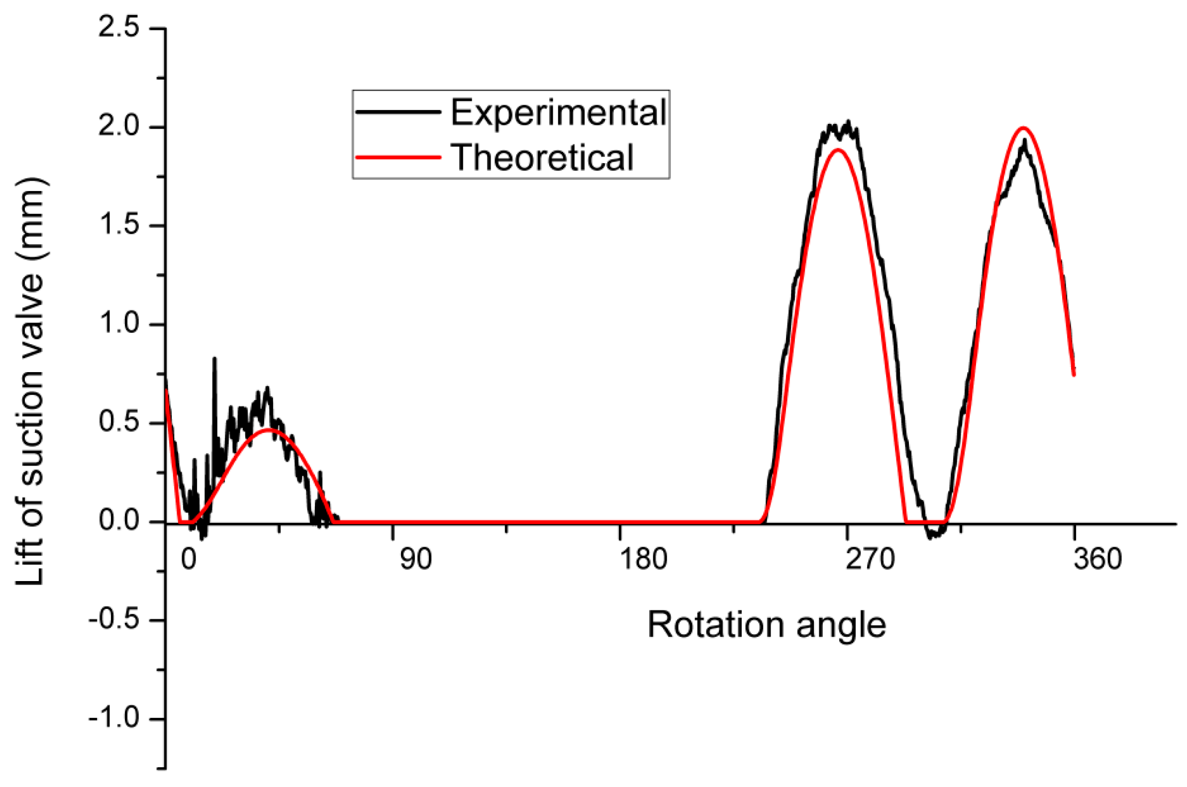
The valve motion and mass flow rate are coupled. The valve motion is mainly governed by the differential pressure between the cylinder and the suction and exhaust, and the valve dynamics also affect the flow and hence the mass flow rate of the refrigerant. As a result, the valve motion is a critical factor to study the thermal cycle in the cylinder.
Figure 12 shows the comparison of theoretical and experimental lift of suction valve in the suction phase, and the numerical calculation is proved to be acceptable.
4.2. Effect of Rotating Speed on the Backflow Phase
The backflow phase of the compressor was studied under variable speed conditions which are necessary for the inverter refrigerator compressor.
The m-θ diagram at different rotating speed is shown in Figure 13 under constant operating conditions. The refrigerant mass in cylinder of expansion phase rises first and then falls with increasing speed. This indicates that mass in cylinder of compression phase depends not only on the backflow through the suction valve but also the flow velocity through the suction valve.
The difference of the refrigerant mass at the maximum cylinder volume (184.32°) is mainly due to different suction flow losses at different speeds. The less refrigerant mass in the expansion phase and the more refrigerant mass in the compression phase, the more favorable it is for compressor efficiency.
The six angular position of split points (reference Figure 6) for the six phases are listed in Table 3. The start/end position and durations of each phase can be obtained from this table.
The expansion and compression phase are relatively independent and the two processes are investigated separately.
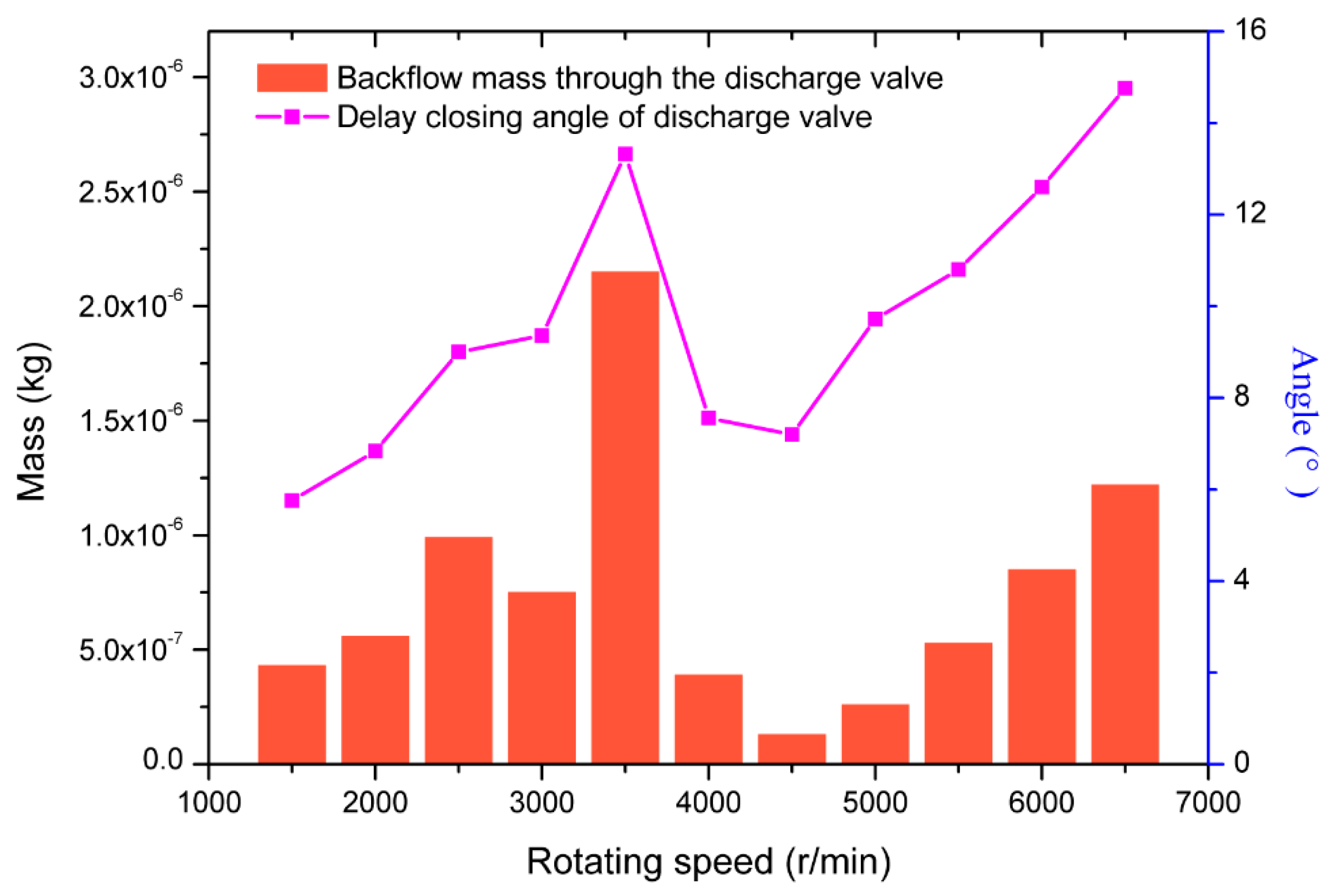
The Figure 14 showed the variation of backflow suction mass with respect to different speed, which is consistent with the variation of delayed closure time of suction valve at different speeds calculated from Table 3. This indicates that delayed closure of suction valve leads to the refrigerant flowing out the cylinder in backflow phase. In this study, the delay time of the suction valve at 5500 r·min−1 is the longest corresponding to the maximum backflow.
This is related to the inherent characteristics of the suction valve, and this peak point can be optimized by changing the stiffness and mass of the suction valve.
As for the backflow phase through the discharge valve, as shown in the Figure 15, the backflow mass also follows the same trend in that the delayed closure time increases with the increase of speed. The delayed closure of discharge valve leads to refrigerant mass increase in the expansion phase which is detrimental to the flow rate of compressor. The delay time of discharge valve is the longest at the speed of 3500 r·min−1. Again, this could be optimzied by changing the inherent characteristics of the discharge valve.
Based on the analysis of m-θ diagram under different speed, the backflow through the valve depends on the delayed valve closure. Due to the characteristics of the valve, it has the maximum backflow at a specific speed. When lower than the specific speed (for example, at 1500 r·min−1 for both the suction valve and discharge valve), the valve has a longer flow time, enough to allow for timely suction and discharge of the refrigerant. When higher than the specific speed, due to the higher flow speed and the larger pressure difference between the two sides of the valve, the refrigerant could be sucked in and discharged in a timely manner.
5. Conclusions
The variation of refrigerant mass in the cylinder has been studied using the m-θ diagram approach. As the first report on this topic, this study discloses the key method to optimize the compressor and the control strategy to improve energy efficiency. The following conclusions are drawn:
- This paper proposed using the m-θ diagram, which focuses on the variation of refrigerant mass in the cylinder with the crank angle to study the flow characteristics of the refrigerator compressor. The m-θ diagram could directly indicate the mass flow rate of refrigerant and the backflow of refrigerant caused by the delayed closure of the valve.
- To improve the thermodynamic model, the flow coefficient of the valve is obtained based on the FSI model, which is more reasonable and accurate compared to the conventional empirical flow coefficient.
- Based on the m-θ diagram, the speed has a great influence on the backflow phase, which depends on the movement of the valve. For a given characteristic of valve, the valve has a peak backflow at a specific speed.
Author Contributions
Zhilong He and Tao Wang conceived and designed the study. Tao Wang and Jun Guo performed the experiments. Tao Wang wrote the paper. Xueyuan Peng and Zhilong He reviewed and edited the manuscript. All authors read and approved the manuscript.
Conflicts of Interest
The authors declare no conflict of interest.
Nomenclature
| m | Refrigerator mass in cylinder |
| θ | Crank angle |
| ω | Angular velocity |
| e | Eccentric distance |
| Vc | The volume of cylinder |
| Vs | The volume of suction chamber |
| Vd | The volume of discharge chamber |
| V0 | Clearance volume |
| D | Cylinder diameter |
| r | Rotating radius |
| λ | Crank-Link Rod Ratio |
| min | Mass through the suction valve |
| mout | Mass through the discharge valve |
| ml | Leakage mass |
| p | Pressure |
| v | Specific volume |
| β | Flow coefficient of the valve |
| A | Valve clearance area |
| k | The adiabatic exponent |
| γ | Nozzle pressure ratio |
| Mv | Equivalent mass of reed valve |
| Kv | Equivalent stiffness of reed valve |
| fs,d | Natural frequency |
| α | Dimensionless displacement of valve |
| Y | Dimensionless velocity of valve |
| ξ | Damping coefficient |
| C | Thrust coefficient of valve |
| Av | Effective area of valve |
| Δp | Pressure difference on valve |
| μ | Oil viscosity |
| d2 | The diameter of valve head |
| d1 | The diameter of valve hole |
| x | Valve displacement |
References
- Ribas, F.A., Jr.; Deschamps, C.J.; Fagotti, F.; Morriesen, A.; Dutra, T. Thermal Analysis of Reciprocating Compressors—A Critical Review. In Proceedings of the 19th International Compressor Engineering Conference at Purdue, West Lafayette, IN, USA, 17–20 July 2006; p. 1306. [Google Scholar]
- Possamai, F.C.; Todescat, M.L. A review of household compressor energy performance. In Proceedings of the 17th International Compressor Engineering Conference at Purdue, West Lafayette, IN, USA, 12–15 July 2004; p. C076. [Google Scholar]
- Morriesen, A.; Deschamps, C.J. Experimental investigation of transient fluid flow and superheating in the suction chamber of a refrigeration reciprocating compressor. Appl. Therm. Eng. 2012, 41, 61–70. [Google Scholar] [CrossRef]
- Costagliola, M. Theory of spring-loaded valves for reciprocating compressors. J. Appl. Mech. Trans. ASME 1950, 17, 415–420. [Google Scholar]
- Si-Ying, S.; Ting-Rong, R. New method of thermodynamic computation for a reciprocating compressor: Computer simulation of working process. Int. J. Mech. Sci. 1995, 37, 343–353. [Google Scholar]
- Stouffs, P.; Tazerout, M.; Wauters, P. Thermodynamic analysis of reciprocating compressors. Int. J. Therm. Sci. 2001, 40, 52–66. [Google Scholar] [CrossRef]
- Pérez-Segarra, C.D.; Rigola, J.; Sòria, M.; Oliva, A. Detailed thermodynamic characterization of hermetic reciprocating compressors. Int. J. Refrig. 2005, 28, 579–593. [Google Scholar] [CrossRef]
- Farzaneh-Gord, M.; Niazmand, A.; Deymi-Dashtebayaz, M.; Rahbari, H.R. Thermodynamic analysis of natural gas reciprocating compressors based on real and ideal gas models. Int. J. Refrig. 2015, 56, 186–197. [Google Scholar] [CrossRef]
- Dutra, T.; Deschamps, C.J. A simulation approach for hermetic reciprocating compressors including electrical motor modeling. Int. J. Refrig. 2015, 59, 168–181. [Google Scholar] [CrossRef]
- Stiaccini, I.; Galoppi, G.; Ferrari, L.; Ferrara, G. A reciprocating compressor hybrid model with acoustic FEM characterization. Int. J. Refrig. 2016, 63, 171–183. [Google Scholar] [CrossRef]
- Liu, G.; Zhao, Y.; Tang, B.; Li, L. Dynamic performance of suction valve in stepless capacity regulation system for large-scale reciprocating compressor. Appl. Therm. Eng. 2016, 96, 167–177. [Google Scholar] [CrossRef]
- Ma, Y.; He, Z.; Peng, X.; Xing, Z. Experimental investigation of the discharge valve dynamics in a reciprocating compressor for trans-critical CO2 refrigeration cycle. Appl. Therm. Eng. 2012, 32, 13–21. [Google Scholar] [CrossRef]
- Nagata, S.; Nozaki, T.; Akizawa, T. Analysis of dynamic behavior of suction valve using strain gauge in reciprocating compressor. In Proceedings of the International Compressor Engineering Conference at Purdue, West Lafayette, IN, USA, 12–15 July 2010. [Google Scholar]
- Real, M.A.; Pereira, E.A.G. Using PV diagram synchronized with the valve functioning to increase the efficiency on the reciprocating hermetic compressors. In Proceedings of the International Compressor Engineering Conference at Purdue, West Lafayette, IN, USA, 12–15 July 2010. [Google Scholar]
- Semlitsch, B.; Wang, Y.; Mihăescu, M. Flow effects due to valve and piston motion in an internal combustion engine exhaust port. Energy Convers. Manag. 2015, 96, 18–30. [Google Scholar] [CrossRef]
Figure 1.
The thermodynamic model of the refrigerator compressor.
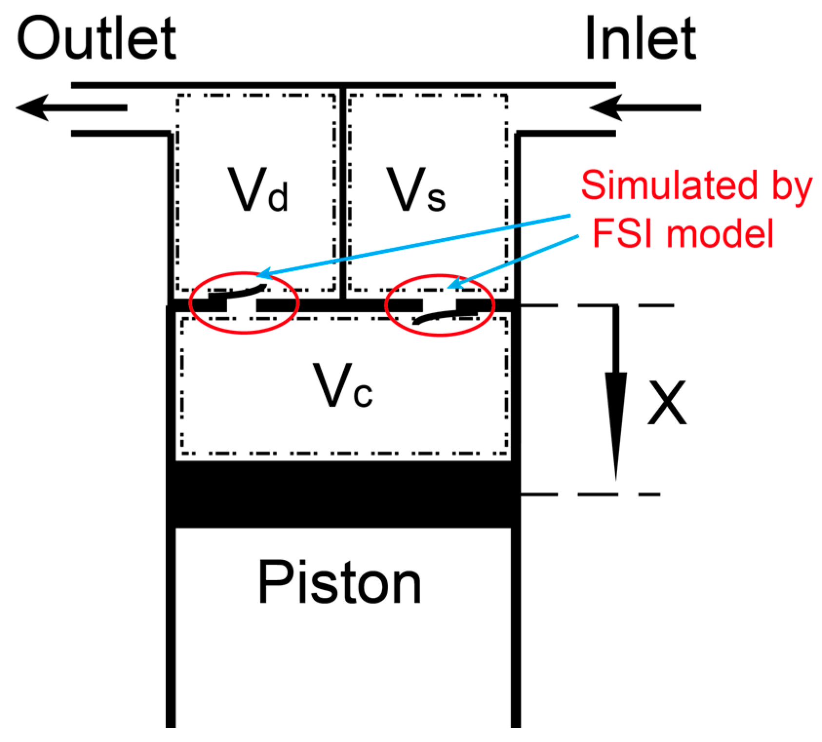
Figure 2.
FSI model of the flow through suction reed valve.

Figure 3.
Flow coefficient of suction valve calculated by the FSI model.

Figure 4.
Flow coefficient of discharge valve calculated by the FSI model.

Figure 5.
Flow chart for thermodynamic model of refrigerator compressor.
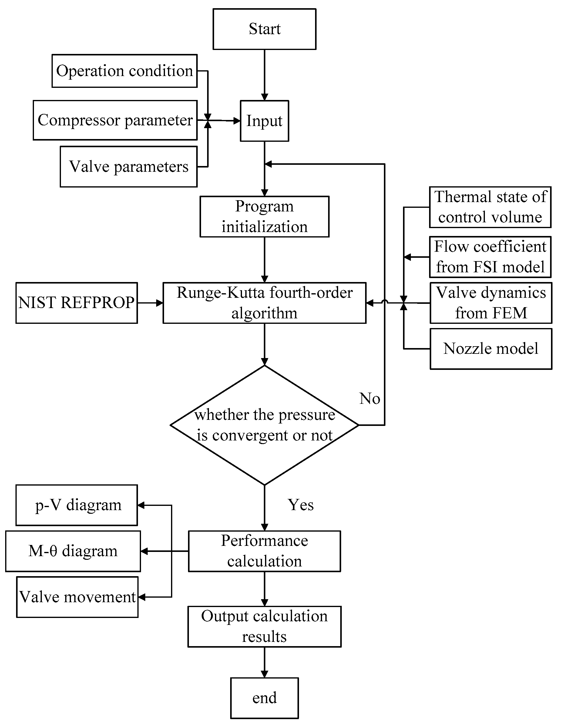
Figure 6.
Details of the m-θ diagram.
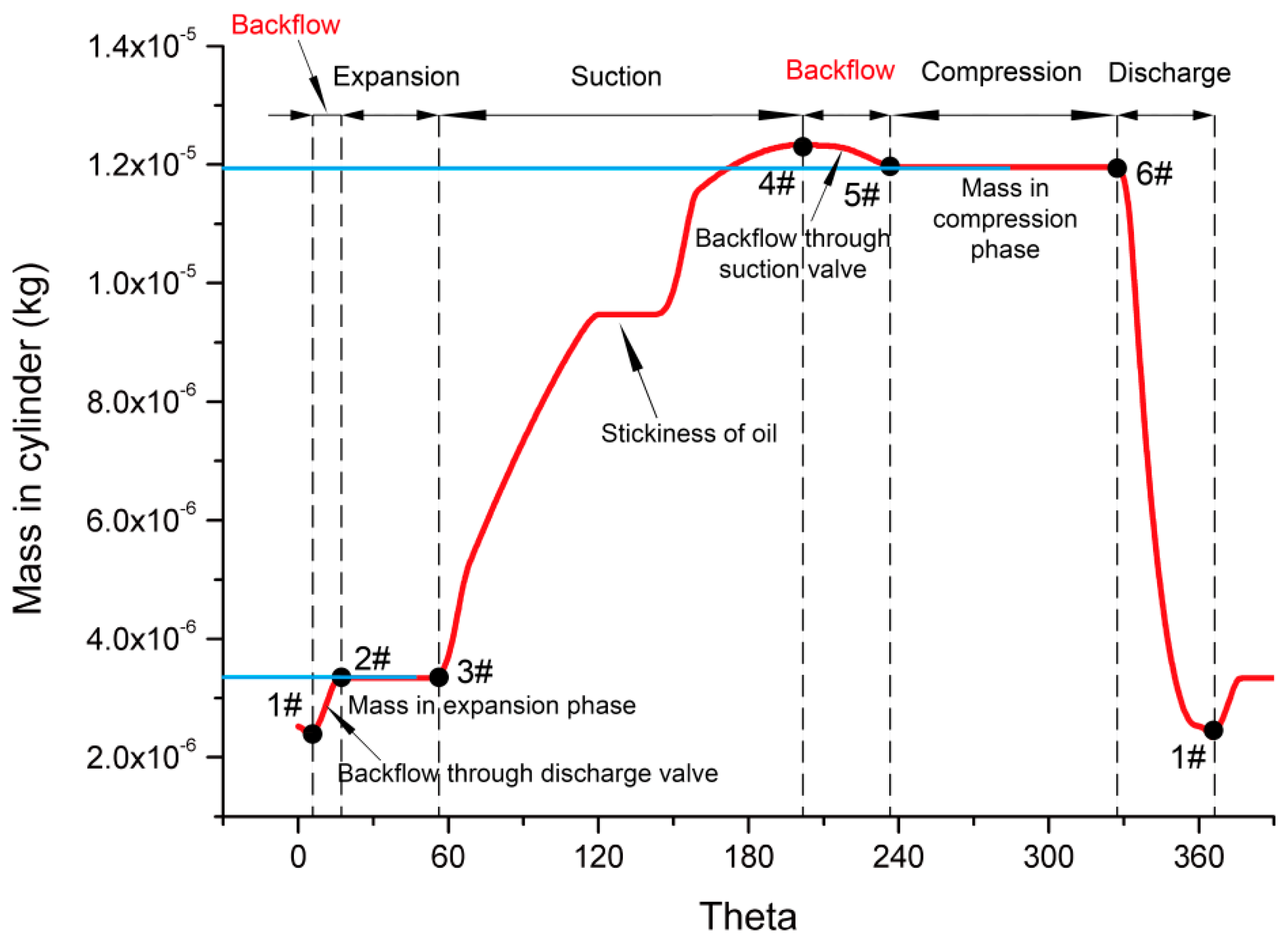
Figure 7.
Schematic of the modified compressor.
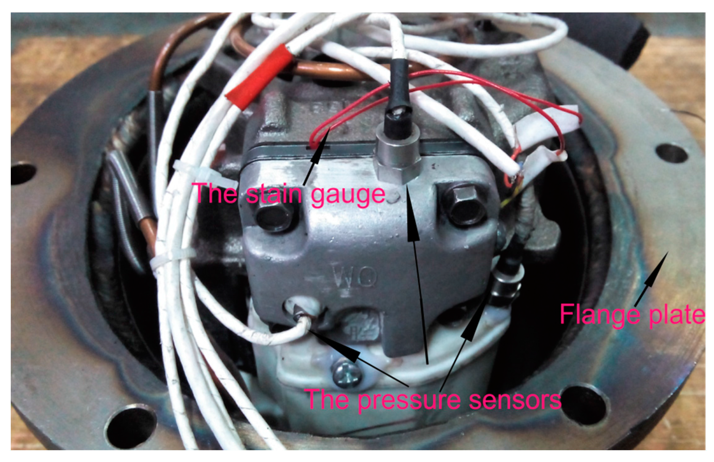
Figure 8.
The installation of the pressure sensor.
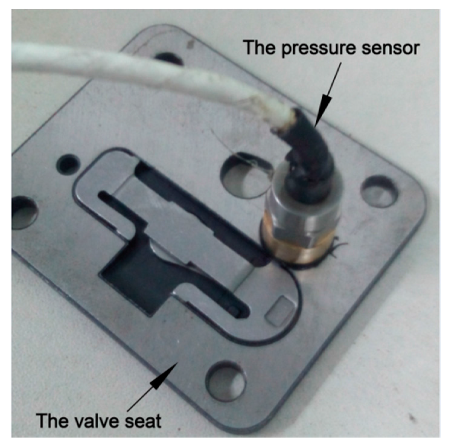
Figure 9.
Schematic of the strain gauge installation.

Figure 10.
Test facility for refrigeration system: (a) Refrigeration system; (b) An evaporator and other additional components.
Figure 10.
Test facility for refrigeration system: (a) Refrigeration system; (b) An evaporator and other additional components.

Figure 11.
Comparison of the experimental and calculated p-V indicator diagram.
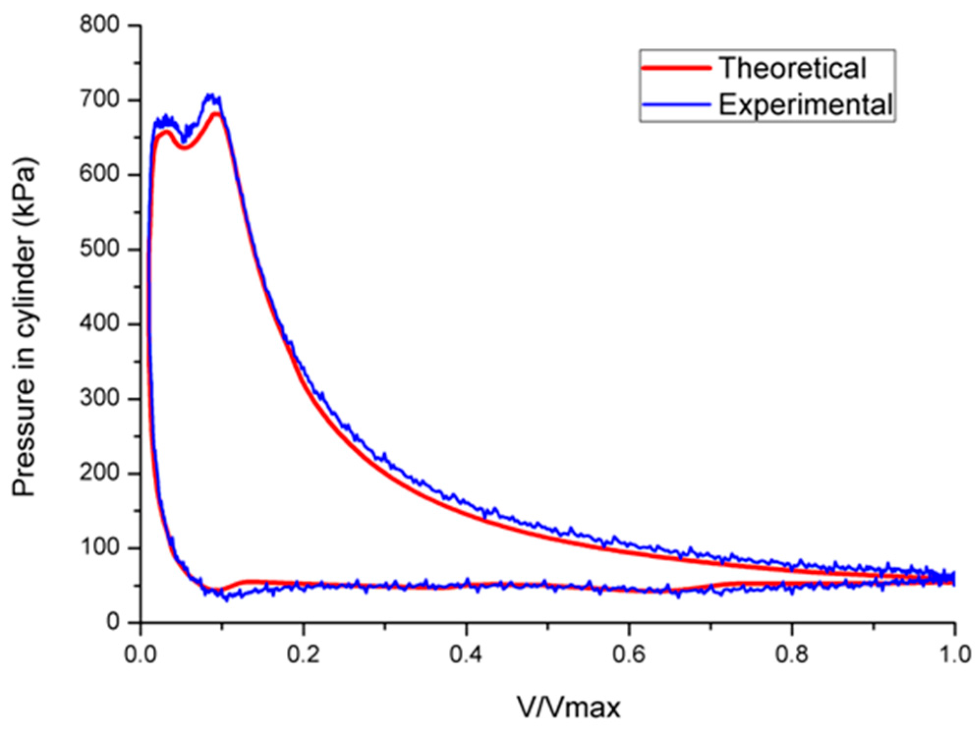
Figure 12.
Comparison of the experimental and calculated lift of suction valve.

Figure 13.
The m-θ diagram under different rotating speed.
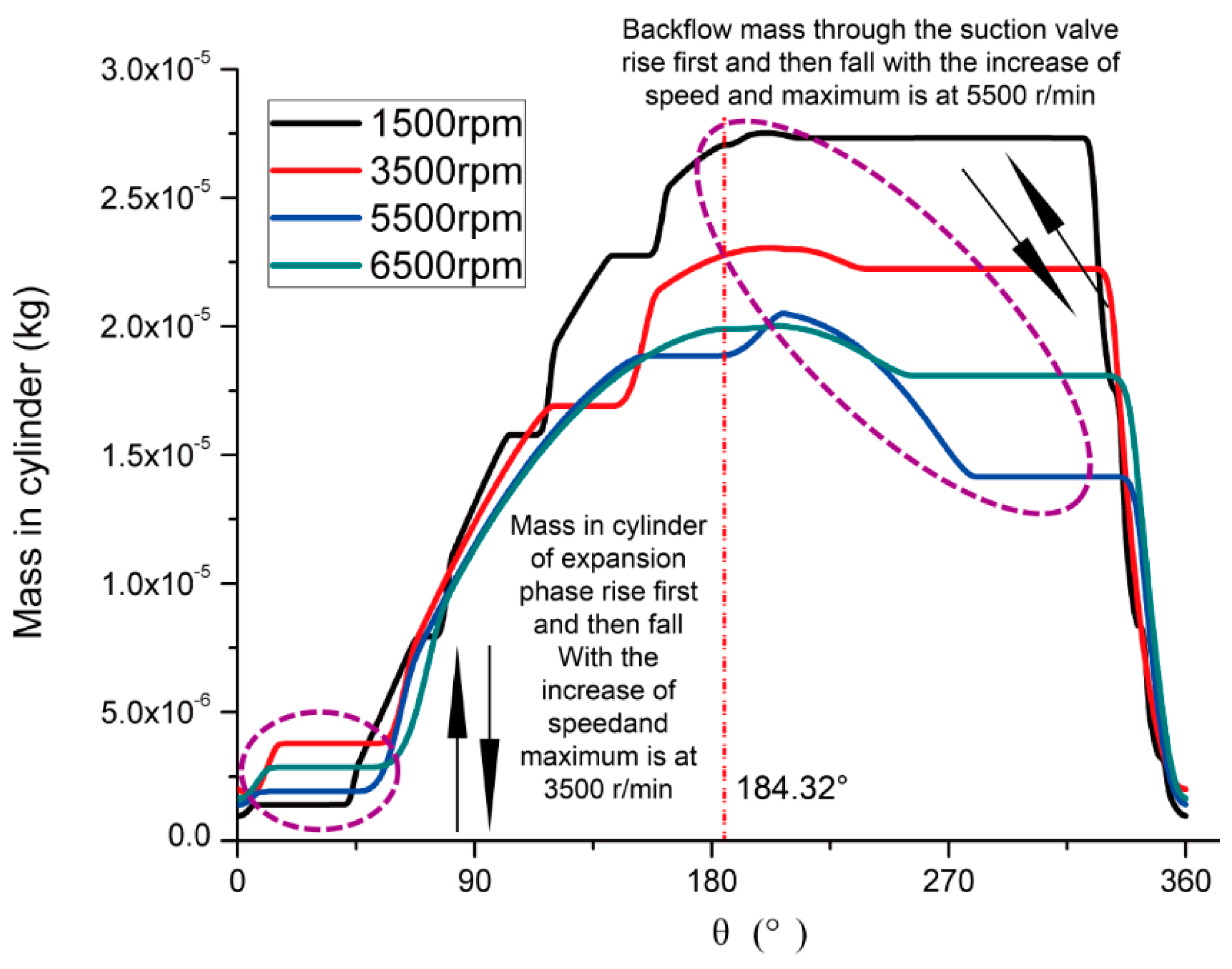
Figure 14.
The backflow and the delay closure of suction valve under different rotating speed.
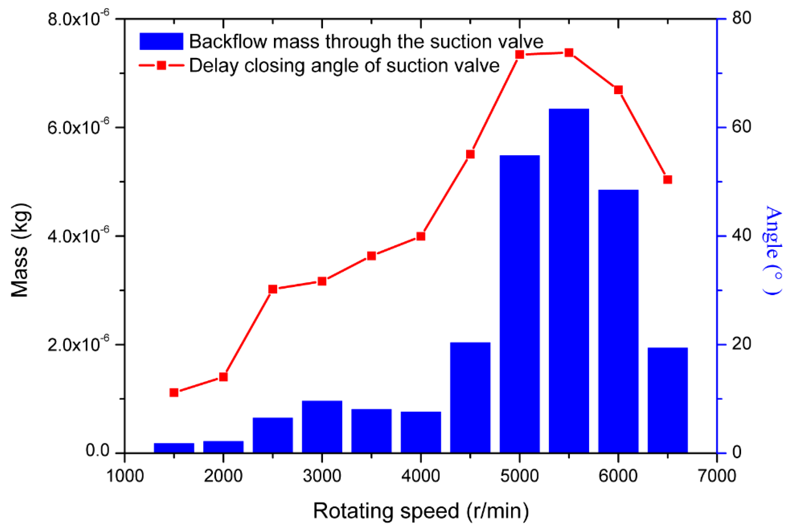
Figure 15.
The backflow and the delay closure of discharge valve under different rotating speed.

Table 1.
Stiffness, natural frequency and equivalent mass of the valves.
| Valve | Natural Frequency(Hz) | Equivalent Mass (g) | Equivalent Stiffness (N/m) | |
|---|---|---|---|---|
| Simulation | Experiment | |||
| Suction valve | 182.39 | 179.73 | 0.9244 | 193.21 |
| Discharge valve | 332.24 | / | 0.4651 | 322.58 |
Table 2.
The structural parameters of the refrigerator compressor.
| Compressor Parameters | Value |
|---|---|
| Cylinder diameter | 31 mm |
| Connecting rod length | 39.5 mm |
| Crank radius | 12 mm |
| Rated speed | 2950 r·min−1 |
Table 3.
The angle of split points for the six phases under different rotating speeds.
| Rotation Speed (r·min−1) | 1# ° | 2# ° | 3# ° | 4# ° | 5# ° | 6# ° |
|---|---|---|---|---|---|---|
| 1500 | 0.36 | 6.12 | 34.56 | 200.88 | 212.04 | 321.12 |
| 2000 | 1.08 | 7.92 | 40.68 | 204.12 | 218.16 | 322.92 |
| 2500 | 1.8 | 11.16 | 45 | 204.84 | 235.08 | 324.36 |
| 3000 | 1.44 | 10.44 | 44.64 | 202.68 | 234.36 | 325.08 |
| 3500 | 4.32 | 17.64 | 53.64 | 201.24 | 237.6 | 326.16 |
| 4000 | 2.88 | 10.44 | 45.36 | 201.24 | 241.2 | 327.24 |
| 4500 | 1.08 | 8.28 | 43.92 | 200.52 | 255.6 | 329.4 |
| 5000 | 0.72 | 10.44 | 45 | 203.76 | 277.2 | 333.36 |
| 5500 | 0.72 | 11.52 | 46.8 | 206.28 | 280.08 | 334.8 |
| 6000 | 0.72 | 13.32 | 48.6 | 207.36 | 274.32 | 334.08 |
| 6500 | 0.36 | 15.12 | 51.84 | 205.2 | 255.6 | 331.2 |
© 2017 by the authors. Licensee MDPI, Basel, Switzerland. This article is an open access article distributed under the terms and conditions of the Creative Commons Attribution (CC BY) license (http://creativecommons.org/licenses/by/4.0/).
Share and Cite
MDPI and ACS Style
Wang, T.; He, Z.; Guo, J.; Peng, X. Investigation of the Thermodynamic Process of the Refrigerator Compressor Based on the m-θ Diagram. Energies 2017, 10, 1517. https://doi.org/10.3390/en10101517
AMA Style
Wang T, He Z, Guo J, Peng X. Investigation of the Thermodynamic Process of the Refrigerator Compressor Based on the m-θ Diagram. Energies. 2017; 10(10):1517. https://doi.org/10.3390/en10101517
Chicago/Turabian StyleWang, Tao, Zhilong He, Jun Guo, and Xueyuan Peng. 2017. "Investigation of the Thermodynamic Process of the Refrigerator Compressor Based on the m-θ Diagram" Energies 10, no. 10: 1517. https://doi.org/10.3390/en10101517
Note that from the first issue of 2016, this journal uses article numbers instead of page numbers. See further details here.