Building Energy Consumption Prediction: An Extreme Deep Learning Approach


1
School of Information and Electrical Engineering, Shandong Jianzhu University, Jinan 250101, China
2
Institute of Automation, Chinese Academy of Sciences, Beijing 100190, China
*
Author to whom correspondence should be addressed.
Energies 2017, 10(10), 1525; https://doi.org/10.3390/en10101525
Submission received: 23 August 2017
/
Revised: 25 September 2017
/
Accepted: 25 September 2017
/
Published: 7 October 2017
(This article belongs to the Special Issue Data Science and Big Data in Energy Forecasting)
Abstract
:Building energy consumption prediction plays an important role in improving the energy utilization rate through helping building managers to make better decisions. However, as a result of randomness and noisy disturbance, it is not an easy task to realize accurate prediction of the building energy consumption. In order to obtain better building energy consumption prediction accuracy, an extreme deep learning approach is presented in this paper. The proposed approach combines stacked autoencoders (SAEs) with the extreme learning machine (ELM) to take advantage of their respective characteristics. In this proposed approach, the SAE is used to extract the building energy consumption features, while the ELM is utilized as a predictor to obtain accurate prediction results. To determine the input variables of the extreme deep learning model, the partial autocorrelation analysis method is adopted. Additionally, in order to examine the performances of the proposed approach, it is compared with some popular machine learning methods, such as the backward propagation neural network (BPNN), support vector regression (SVR), the generalized radial basis function neural network (GRBFNN) and multiple linear regression (MLR). Experimental results demonstrate that the proposed method has the best prediction performance in different cases of the building energy consumption.
1. Introduction
Nowadays, with economic growth and the population increasing, more and more energy is consumed. As one aspect of the energy consumption, building energy consumption accounts for a considerable proportion [1,2]. For example, in China, statistical data shows that building energy consumption accounted for 28% of the total energy consumption in 2011, and that it will reach 35% by 2020 [3]; in the United States, building energy consumption is close to 39% of the total energy consumption [4].Therefore, it is necessary to propose some efficient strategies to promote the building energy utilization rate. Building energy consumption prediction can help building managers to make better decisions so as to reasonably control all kinds of equipment. Hence, this is an efficient and helpful way to reduce the consumption of building energy and to improve the energy utilization rate.
A great number of prediction methods have been proposed in the past several decades for building energy consumption prediction. The majority of the case studies depend on the historical energy consumption time series data to construct the prediction models [5]. Generally, the proposed methods for building energy consumption prediction fall into two categories, which are statistical methods and artificial intelligence methods.
The statistical methods utilize the historical data to construct probabilistic models in order to estimate and analyze the future energy consumption. In [6], principal component analysis (PCA) was utilized to select the significant inputs of the energy consumption prediction model. In [7], linear regression was applied to estimate electricity consumption in an institutional building, and moreover, fuzzy modeling and neural networks were chosen as two comparative approaches to evaluate the performance of the linear regression method. In [8], the autoregressive model with extra inputs (ARX) was utilized to estimate the parameters of building components. In [9], Kimbara et al. developed an autoregressive integrated moving average (ARIMA) model to implement online building energy consumption prediction. In [10], the ARIMA with external inputs (ARIMAX) model was applied to predict the power demand of the buildings. In [11], a regression-based method—conditional demand analysis (CDA)—was used for predicting the building energy consumption.
Generally speaking, the artificial intelligence methods can obtain more accurate prediction results in most real-world applications and have been widely applied to the prediction of building energy consumption. In [12], clusterwise regression, a novel technique that integrates clustering and regression simultaneously was proposed for forecasting building energy consumption. In [13], a clustering method was proposed to find the similarity of pattern sequences for electricity prices and demand prediction. In [14], a k-means method was presented for analyzing the pattern of electricity consumption in buildings. Additionally, data mining techniques applied to electricity-related time series forecasting were surveyed in [15]. In [16], a decision tree was used to understand the energy consumption patterns and to forecast the energy consumption levels. In addition, in [17], a random forest (RF) was used to help facility managers to improve the energy efficiency in buildings. In [18], a support vector machine (SVM) was utilized to predict the energy consumption of low-energy buildings with a relevant data selection method. Artificial neural networks (ANNs) play an important role in the forecasting of building energy consumption, and different kinds of ANNs have been given for this application. In [19], a short-term predictive ANN model for electricity demand was developed for the bioclimatic building. In [20], the Levenberg–Marquardt and Output-Weight-Optimization (OWO)-Newton algorithm-based ANN was utilized to forecast the residential building energy consumption. In [21,22], the ANN combined with a fuzzy inference system was examined by the building energy consumption prediction. In [23], two adaptive ANNs with accumulative training and sliding window training were proposed for real-time online building energy prediction. In [24], an ANN trained by the extreme learning machine (ELM) was proposed to estimate the building energy consumption and was compared with the genetic algorithm (GA)-based ANN. Furthermore, a hybrid method, the radial basis function neural network (RBFNN), combined with the particle swarm optimization (PSO) algorithm was used to improve the building energy efficiency in [25]. Although the statistical methods and the existing artificial intelligence methods can give satisfactory results, it is still a challenging task to obtain accurate prediction results because of random characteristics that can be affected by the weather, the working hours, the human distribution and the equipment in the buildings. On the other hand, the deep learning techniques that have emerged in recent years provide us with a powerful tool to achieve better modeling and prediction performance. The deep learning algorithm uses deep architectures or multiple-layer architectures adopting the layerwise pre-training method for parameter optimization to obtain great feature learning ability [26]. The inherent features of data extracted from the lowest level to the highest level of the deep learning model are more representative than for the traditional shallow neural network. Hence, the deep architectures have greatly improved performance for the modeling, classification and visualization problems, and they have found lots of applications. In [27], a single convolutional neural network architecture with a multitask learning strategy was designed for natural language processing (NLP). In [28], the deep autoencoder network was utilized to convert high-dimensional data to low-dimensional codes, and experiments demonstrated that it works much better than PCA for dimensionality reduction. In [29], a stacked autoencoder (SAE) was applied for organ identification in medical magnetic resonance images. The deep learning approaches have also been applied to time series prediction problems. In [30], an ensemble deep learning approach was utilized for time series predictions of seven small-batch data sets. In [31], a SAE-based deep neural network (DNN) was constructed to approximate the Q-function in the reinforcement learning of traffic signal timing. In [32], a SAE was utilized to realize the traffic-flow prediction on the basis of traffic-flow time series. Additionally, in [33], a deep learning-based approach for time series forecasting with an application to electricity load was given. In all these applications, the experimental results demonstrated that the deep learning approaches can outperform the comparative methods.
Compared with the data sets in the research domains of image recognition, speech recognition, and machine vision, for example, the data sets in the time series prediction applications [30,31,32,33] do not have a large quantity of data. However, in these applications, the deep learning approaches, including the SAE approach, still performed better than some traditional machine learning methods because of the relatively deeper architectures and the improved or newly proposed learning strategies in the deep learning approaches. In this paper, to enhance the prediction performance, we propose an extreme deep learning approach to estimate building energy consumption. The proposed approach combines the SAE with the ELM to make full use of their respective advantages. The SAE is used to extract the building energy consumption features. Additionally, the ELM is utilized as a predictor to obtain accurate prediction results. In the proposed extreme SAE approach, only the pre-training of the SAE is needed, while the fine-tuning of the whole network is replaced by least-squares learning of the parameters in the last fully connected layer. In addition, in order to determine reasonable input variables for the extreme deep learning model, the partial autocorrelation analysis method is adopted in this application. Finally, the proposed approach is compared with some popular methods, such as the backward propagation neural network (BPNN), support vector regression (SVR), the generalized radial basis function neural network (GRBFNN) and multiple linear regression (MLR). The experimental results demonstrate that the proposed deep learning model has the best prediction ability for both the 30 and 60 min experiments.
The rest of this paper is organized as follows. In Section 2, the mechanisms of the autoencoder and the SAE are reviewed, and the extreme deep learning model is presented. In Section 3, the prediction model for building energy consumption is discussed in detail. Two experiments on the prediction of the 30 and 60 min building energy consumption have been performed and the experimental results are given in Section 4. Finally, the conclusions of this paper are drawn in Section 5.
2. Methodology
In this section, the structure and learning mechanism of the SAE is introduced first. Then, the extreme deep architecture is shown, and the parameter learning algorithm is given.
To begin, we assume that there are N input–output training data pairs , where is the input part with n input variables and is the output part with only one output variable.
2.1. The Stacked Autoencoder
The SAE uses multiple autoencoders as building blocks to construct a DNN [34]. Hence, before the introduction of the SAE, the autoencoder is described first.
2.1.1. Autoencoder
The autoencoder is an unsupervised neural network and is composed of three layers which are the input layer, the hidden layer, and the output layer [28]. It attempts to dig out a limited number of representations to reconstruct its input, that is, the target output is equal to the input of the model. The structure of one autoencoder with L hidden nodes is demonstrated in Figure 1.
In the autoencoder, there are two processes—the encoding process and the decoding process. In the encoding process, an autoencoder attempts to dig out a hidden representation , which can be computed as
where is an encoding matrix, is an encoding bias vector, and is the activation function that can be chosen as the sigmoid function or the tanh function.
Additionally, in the decoding process, a decoding matrix needs to be determined to decode the hidden representation back into a reconstruction . The decoded output can be computed as
where and are respectively the decoding matrix and the decoding bias vector, and again, is the activation function that can be chosen as the sigmoid function or the tanh function.
We always expect the error between the input and the reconstruction to be as small as possible. This can be achieved by minimizing the following loss function [35]:
In other words, the optimal parameter set of the autoencoder can be determined by solving the following optimization problem:
In the autoencoder, this optimization problem is often solved using one of the variants of the back-propagation algorithm, such as the conjugate gradient method or the steepest descent method, for example.
2.1.2. Sparse Autoencoder
The autoencoder will be invalid for dimension reduction and key feature extraction if the number of hidden nodes is the same or greater than the number of input nodes, that is, . To solve this problem, sparsity constraints are imposed on the hidden layer to obtain the representative features and to learn useful structures from the input data [36,37,38,39]. This allows for sparse representations of inputs and is useful for pre-training in many tasks.
The autoencoder with sparsity constraints is called the sparsity autoencoder. We minimize the following loss function, which imposes a sparsity constraint on the reconstruction error to obtain the optimal parameters of the sparsity autoencoder [36,37,38,39]:
where is the penalty coefficient, is a sparsity parameter that is typically a small value close to zero, is the average activation of the jth hidden node with respect to the training set, and is the Kullback–Leibler divergence, which is also called the relative entropy and is defined as follows [36,37,38,39]:
If , will be zero. Additionally, if is close to 0 or 1, will be infinity.
2.1.3. The Structure of the Stacked Autoencoder
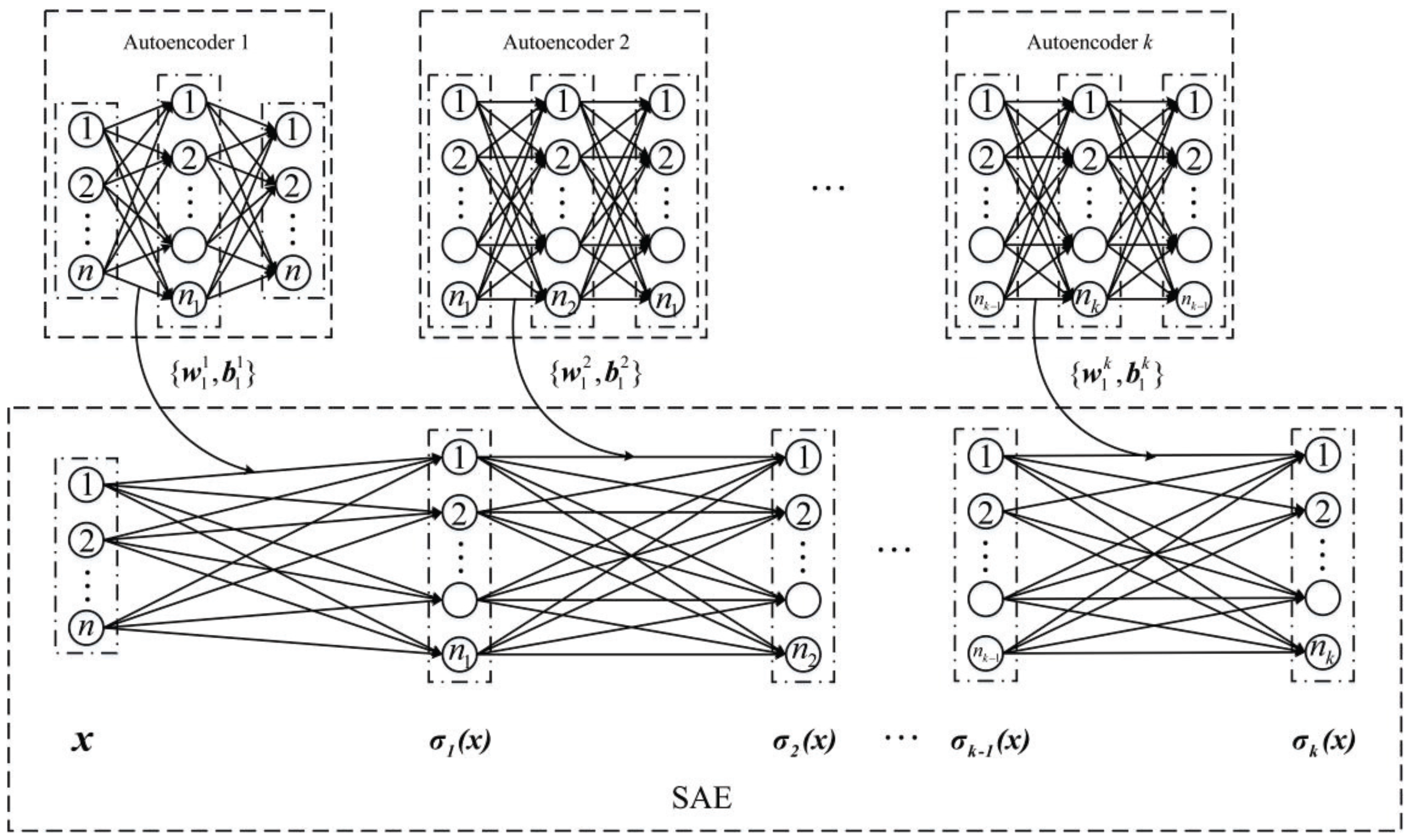
The SAE model as a novel deep learning model is a stack of multiple autoencoders [32,40]. Figure 2 demonstrates the structure of the SAE with k hidden layers. The final output of its last hidden layer can be expressed as
where and are respectively the encoding matrix and the encoding bias vector of the lth autoencoder. Additionally, the activation function can be chosen as the sigmoid or tanh function.
The parameter learning algorithm of the SAE is not mentioned in this subsection; it is introduced in next subsection in detail.
2.2. Extreme Stacked Autoencoder and Its Training Algorithm
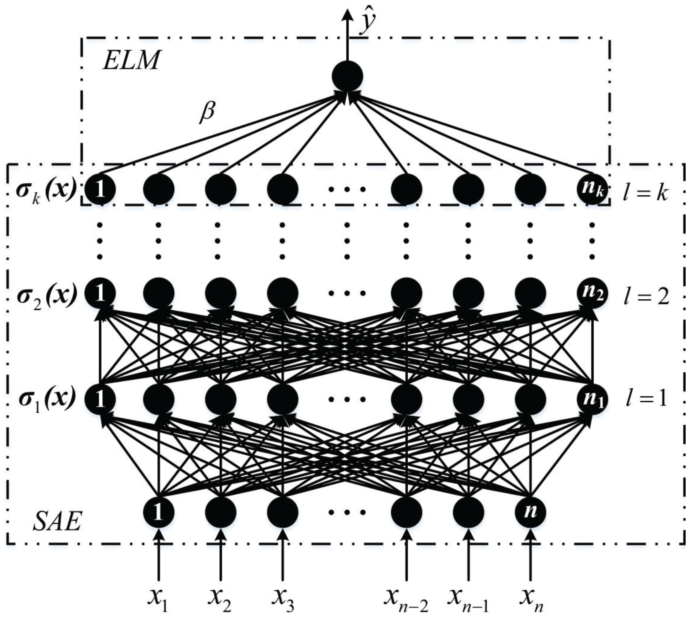
For predicting building energy consumption, we propose a deep learning approach, named extreme SAE, which combines the SAE with the ELM. The structure of the proposed extreme SAE is demonstrated in Figure 3. In this approach, the inputs are given to the SAE part, following which, the fully connected layer is trained by the ELM. The SAE part is used to extract building energy consumption features, while the ELM part is utilized as a predictor to obtain accurate prediction results.
To design an extreme SAE that performs well, optimal parameters, including the parameters in the SAE part and the parameters in the ELM part, should be determined first. In this study, we use two steps to determine these parameters. In the first step, we pre-train the parameters in the SAE part. Then, in the second step, we utilize the least-squares method to find the parameters in the ELM part.
2.2.1. Pre-Training of the Stacked Autoencoder Part
To obtain the optimal parameters of the SAE part, the gradient-based Back-propagation (BP) optimization algorithm is typically used. However, its performance is unsatisfactory, mainly because of the gradient divergence. In order to solve this issue, Hinton et al. have proposed a greedy layerwise unsupervised learning algorithm that can train DNNs successfully [26]. The novel point of this approach is that it pre-trains the SAE model layer by layer in a bottom-up way, as expressed below.
- Step 1: Train the first layer as an autoencoder by minimizing Equation (3) using the training samples as the input, and let .
- Step 2: Train the vth layer by minimizing Equation (3) using as its input.
- Step 3: Let , and iterate Step 2 until .
- Step 4: Output and use it as the input of the predictor.
Here, is the hidden representation of the th layer, and k is the desired number of hidden layers.
2.2.2. Least-Squares Learning of the Extreme Learning Machine Part
In the ELM part, the least-squares method is adopted to optimize the output weighting vector .
From Figure 3, the input data , corresponds to a known hidden representation when all , are determined. We always expect that each of the estimated results with respect to can approximate the true value with no errors. This can be mathematically expressed as
where .
Then, Equation (8) can be rewritten as
where is the output matrix of the SAE as well as the input matrix of the ELM and can be expressed as
According to the knowledge of matrix theory, as discussed in the studies on ELM [41,42,43], the optimal vector in Equation (9) can be derived as
where is the Moore–Penrose generalized inverse of .
We note that the traditional layerwise training of the SAE includes two steps, which are the pre-training of the SAE and the fine-tuning of the whole network. Being different to the traditional layerwise training, the extreme SAE approach utilizes the extreme learning of the output weighting vector to replace the fine-tuning process of the whole network.
3. Energy Consumption Prediction Model
In this section, we construct an extreme SAE model for 30 and 60 min building energy consumption prediction. First of all, the applied data set is shown. Then, the energy consumption prediction model is described. Finally, the experimental settings are introduced.
3.1. Applied Data Set
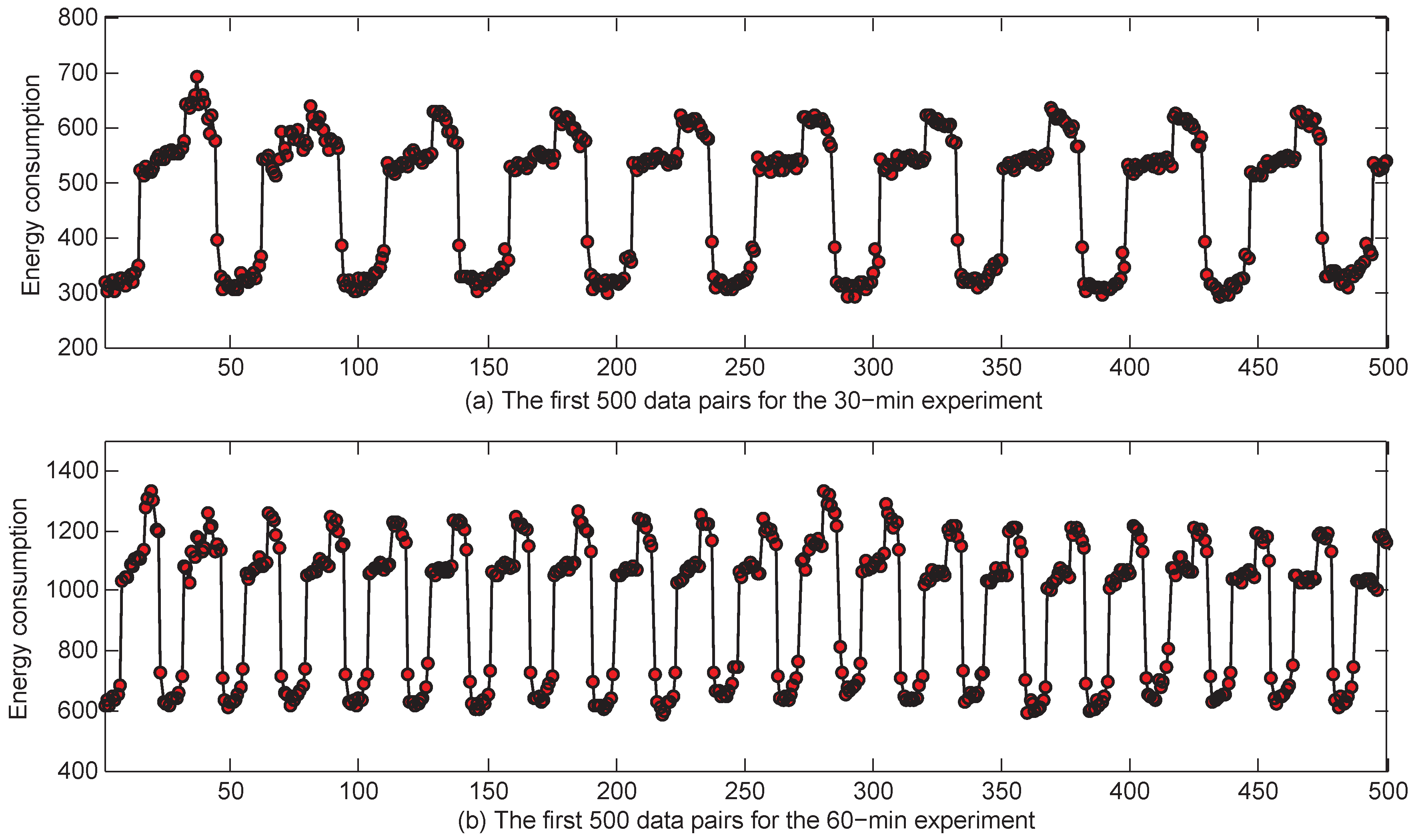
The applied building energy consumption data were download from the website: https://trynthink.github.io/buildingsdatasets/. The data were collected every 15 min in one retail building in Fremont, CA. After the preprocessing of the missing data in the initial data set by the mean filter method, we obtained 34,939 samples in the building energy consumption time series. Then, we aggregated the collected data into 30 and 60 min intervals each for 30 and 60 min predictions. Consequently, the building energy consumption time series for the 30 min experiment had 17,469 data points, and the time series for the 60 min experiment had 8734 data points. For better visualization, we plotted the first 500 samples of the 30 and 60 min cases in Figure 4 rather than plotting the whole time series of the two cases.
3.2. Energy Consumption Prediction Model
In this paper, we utilize n energy consumption data in the building energy consumption time series before time p to predict the value at time p. In other words, we utilize to estimate the value of . Thus, the model for the prediction of energy consumption has the following form:
where represents the prediction model that can be realized by the prediction algorithms.
To be more clear, we assume that the input variables of the prediction models are , where and the output variable is .
To train and test the building energy consumption models, the input–output data pairs should first be formed. Considering the input and output form of the above prediction model, we can obtain the input–output data pairs as follows:
where , , and N is the number of samples in the building energy consumption time series.
The numbers of the input–output data pairs for training and testing are determined by the time lag in different experiments. We give the detailed discussion on this issue below.
3.3. Experimental Setting
As aforementioned, we utilize the extreme SAE to predict the 30 and 60 min building energy consumption. Furthermore, in order to examine the proposed deep learning model’s performance, the BPNN, SVR, the GRBFNN and MLR are chosen as the comparative methods. Below, these comparative methods are introduced briefly.
The BPNN is a multilayer ANN that adopts the back propagation algorithm to train the weights between neighboring layers [44]. This technique has some superior abilities, such as its nonlinear mapping capability, self-learning and adaptive capability, and generalization ability. The BPNN has found lots of applications in many research areas.
In our comparison, SVR is adopted. As one variant of the SVM, SVR still attempts to minimize the generalization error bound so as to achieve generalized performance [45]. Furthermore, the kernel function is utilized in the SVR to avoid the calculations in high-dimensional space. As a result, it can perform well when the input features have high dimensionality.
The GRBFNN is the generalized RBFNN. It utilizes k-fold cross-validation to determine the optimal center and spread of the RBFNN [46]. MLR is the popular statistical method for regression and prediction. It utilizes the ordinary least-squares method or generalized least-squares to minimize the sum of squares of errors (SSE) for obtaining the optimal regression function [47,48].
To examine the effectiveness of the five prediction models, we adopt three performance indices—the mean absolute error (MAE), the mean relative error (MRE), and the root-mean-square error (RMSE), which can be computed respectively as
where K is the number of samples for training or testing, and and are respectively the predicted value and the target value.
In order to guarantee the performance of the prediction models, the input–output data pairs are normalized. In this study, the following equation is used to normalize the input parts of the input–output data pairs:
where , .
4. Experiments
In this section, the 30 and 60 min building energy consumption prediction experiments are analyzed. For each experiment, we determine the optimal input variables for the models first, and then make comprehensive assessments of the five prediction models.
4.1. Thirty Minute Prediction of Building Energy Consumption
4.1.1. Determination of the Optimal Input Variables
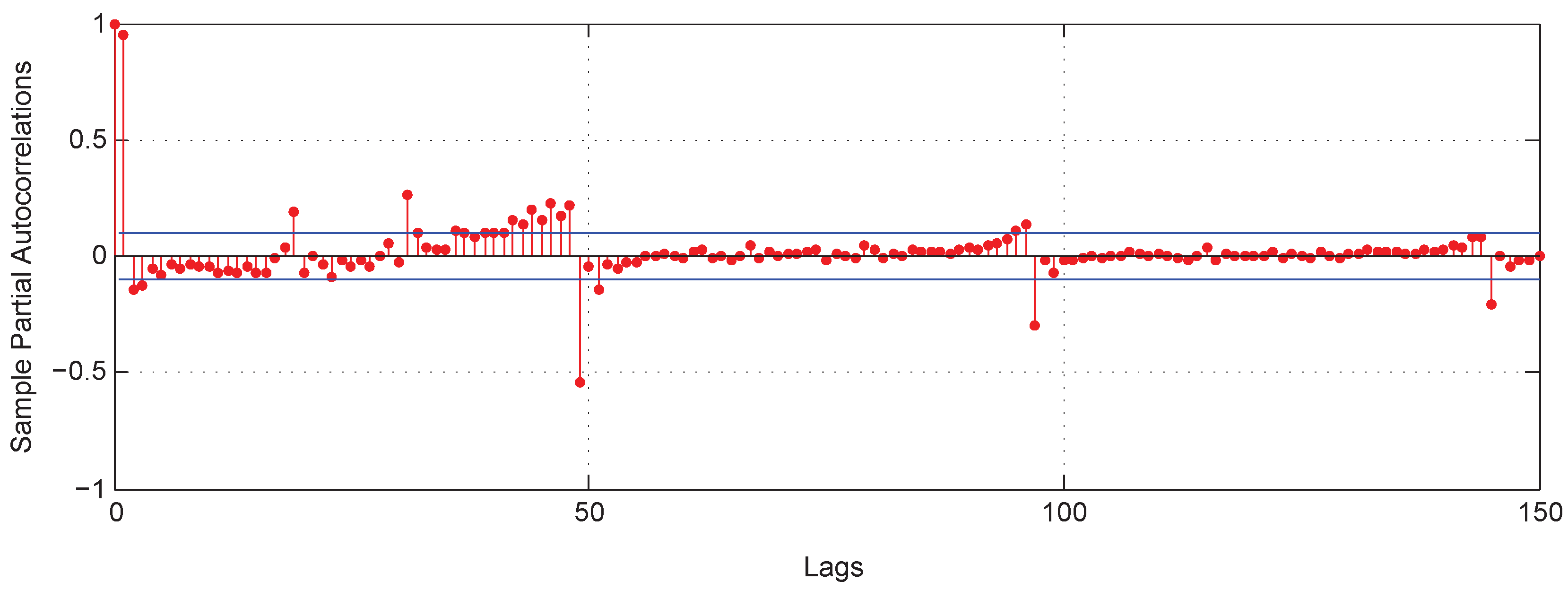
In this study, the partial autocorrelation function (PACF) is adopted to determine the input variables for building energy consumption prediction [49,50]. The PACF can obtain partial autocorrelation between and [51,52]. The greater the partial correlation coefficient, the greater the influence puts on . The PACF of the building energy consumption time series for the 30 min experiment with 150 lags is demonstrated in Figure 5.
To obtain the optimal input variables for predicting building energy consumption, we chose the time series lags whose absolute value of the partial autocorrelations were greater than or equal to 0.1. As shown in Figure 5, for the 30 min experiment, there were 22 lags meeting the above condition. As a result, the determined optimal input variables with respect to are , , , , and .
4.1.2. Configuration of the Prediction Models
For an extreme SAE model that performs well, the number of hidden layers and the number of hidden units in each hidden layer need to be determined.
In this study, we utilized the data pairs generated above to select the optimal structure of the extreme SAE model for the 30 min experiment. Additionally, we assumed that the numbers of hidden units in all hidden layers are equal, that is, , where k is the number of the hidden layers.
In this paper, we chose k from 1 to 4 and the number of hidden units from . In addition, the RMSE index was chosen as the criterion to determine the optimal architectures of the extreme SAE for predicting the building energy consumption.
By performing a grid search, we obtained different RMSEs for the 30 min experiment, and these are shown in Table 1. Clearly, in this case, the extreme SAE with the smallest RMSE has 4 hidden layers and 100 hidden units in each hidden layer.
The parameter configuration of the other four comparative approaches are listed in detail as follows.
For the BPNN, the number of hidden layer nodes and the iteration number were respectively set to be 300 and 15,000. In the hidden layer, the logsig activation function was used. Additionally, in the training process, a gradient descent-based algorithm was adopted.
For SVR, the radial basis function was chosen as the kernel function and the penalty factor C was set to be 50. Moreover, we did not use shrinking heuristics in the training process.
For the GRBFNN, 5-fold cross-validation was adopted to determine the optimal center and spread of the RBF function. In addition, the spread was chosen from 0.01 to 2 with a 0.1 step length.
For MLR, the ordinary least-squares method was adopted to minimize the SSE for obtaining the optimal regression function.
4.1.3. Results
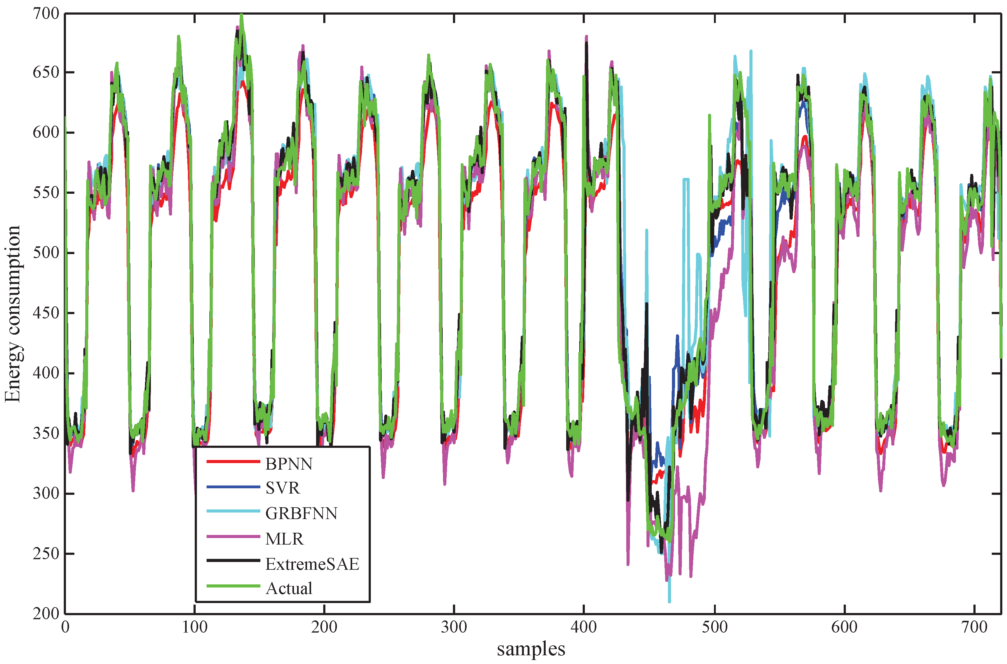
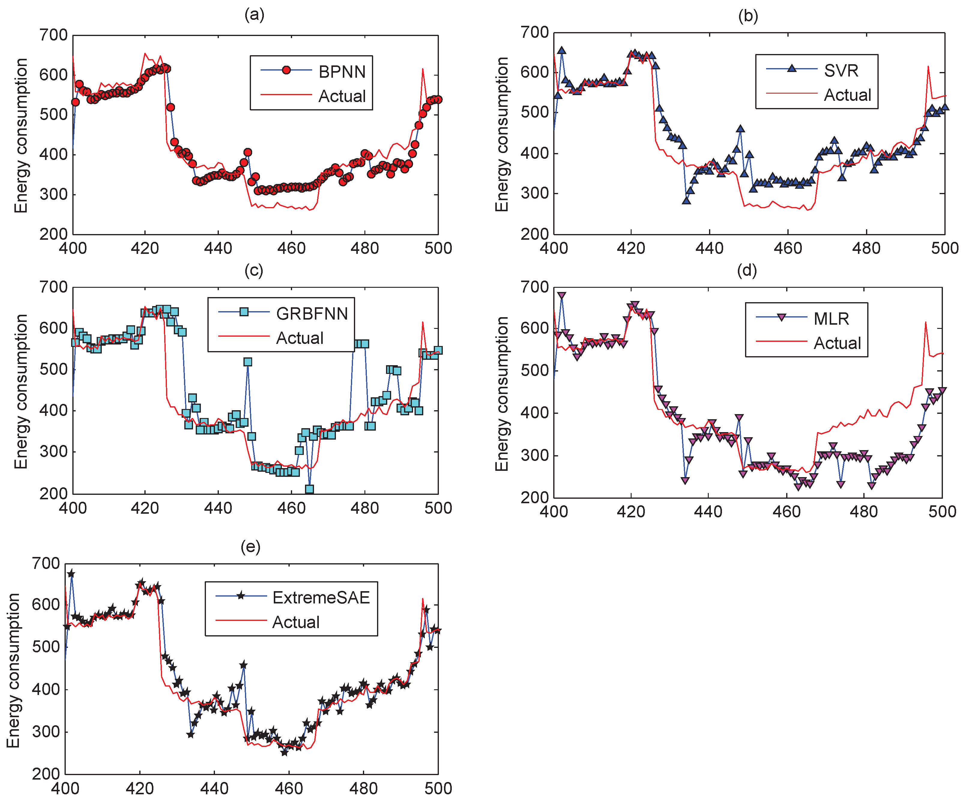
For the testing data, the prediction results of the five prediction models in the 30 min prediction experiment are demonstrated in Figure 6. For better visualization, parts of the results (the values between 400 and 500) in Figure 6 have been zoomed in and are plotted in Figure 7 to show finer details.
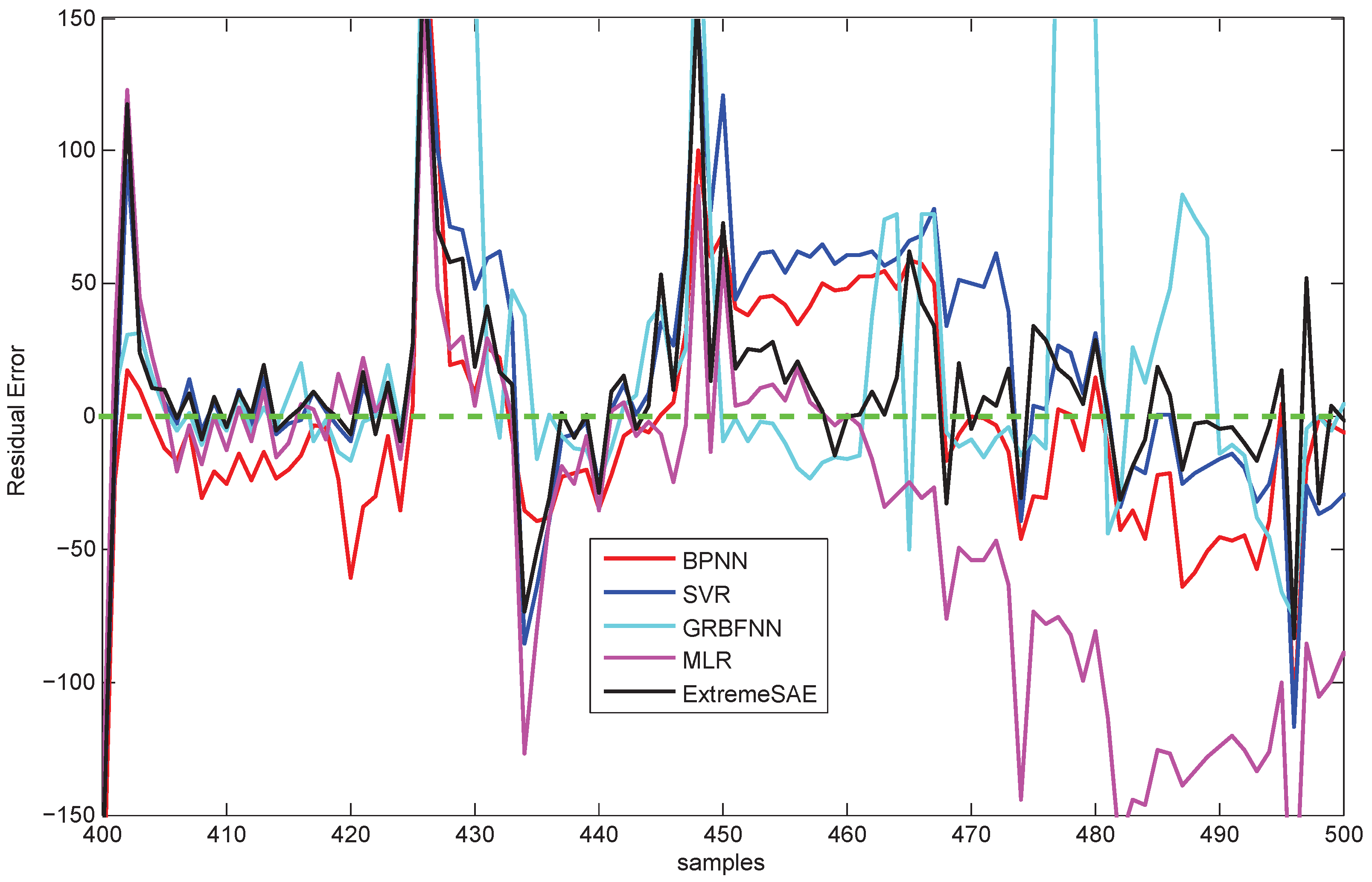
The residual errors of the five prediction models in this 30 min prediction experiment are demonstrated in Figure 8. Similarly, to make for a clear comparison, parts of the results (the values between 400 and 500) in Figure 8 have been zoomed in and are re-plotted in Figure 9.
To quantitatively analyze the performances of the five prediction models, we consider the MAE, MRE and RMSE indices for both the training and the testing processes. For the 30 min prediction, the MAEs, MREs and RMSEs of the five prediction models in the training and testing processes are listed in Table 2.
4.2. Sixty Minute Prediction of Building Energy Consumption
4.2.1. Determination of the Optimal Input Variables
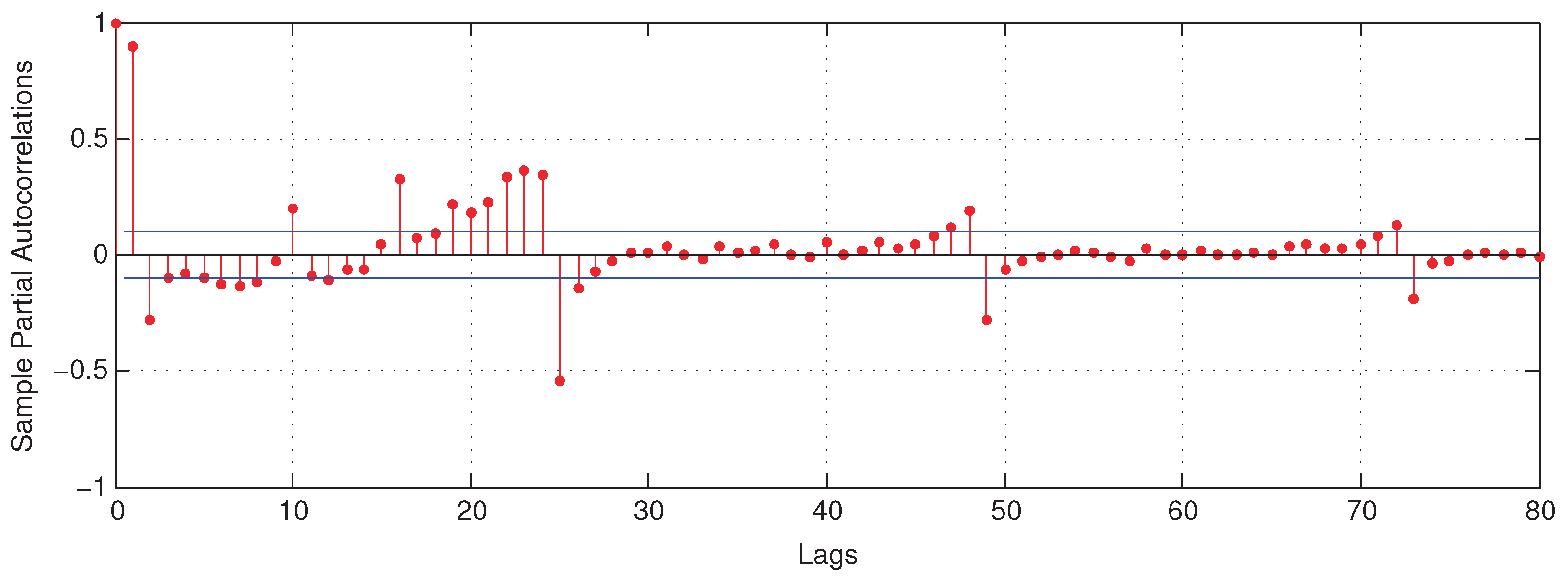
As aforementioned, the PACF was adopted to determine the input variables for building energy consumption prediction. The PACF for the 60 min building energy consumption time series is demonstrated in Figure 10.
We also chose the time series lags whose absolute values of the partial autocorrelations were greater than or equal to 0.1 as the optimal input variables. From Figure 10, for the 60 min building energy consumption prediction, there were 21 lags meeting the above condition. The determined optimal input variables with respect to are , , , , and .
4.2.2. Configuration of the Prediction Models
In the same way as for the 30 min prediction experiment, by performing a grid search, we obtained the values of the RMSEs for the 60 min building energy consumption prediction and list these in Table 3. Clearly, in this case, the extreme SAE with the smallest RMSE has 2 hidden layers and 50 hidden units in each hidden layer.
In this case, the configurations of the BPNN, SVR, the GRBFNN and MLR are as follows. For the BPNN, the number of hidden layer nodes and the iteration number were respectively set to be 200 and 17,000. In the hidden layer, the logsig activation function was used. For SVR, the radial basis function was chosen as the kernel function and the penalty factor C was set to be 80. Again, we did not use shrinking heuristics in the training process. The configurations of the GRBFNN and MLR in this case were the same as those in the 30 min prediction experiment.
4.2.3. Results
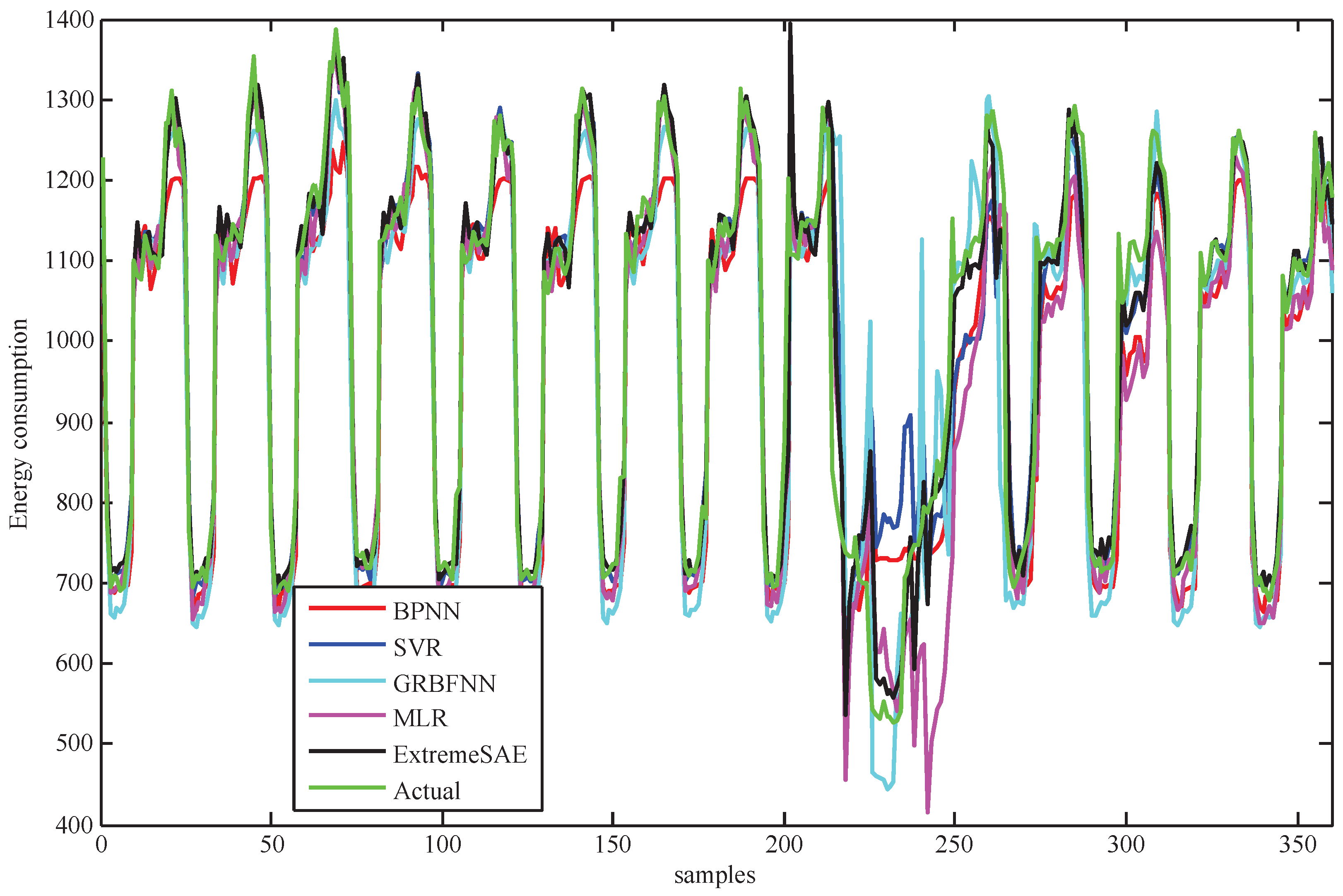
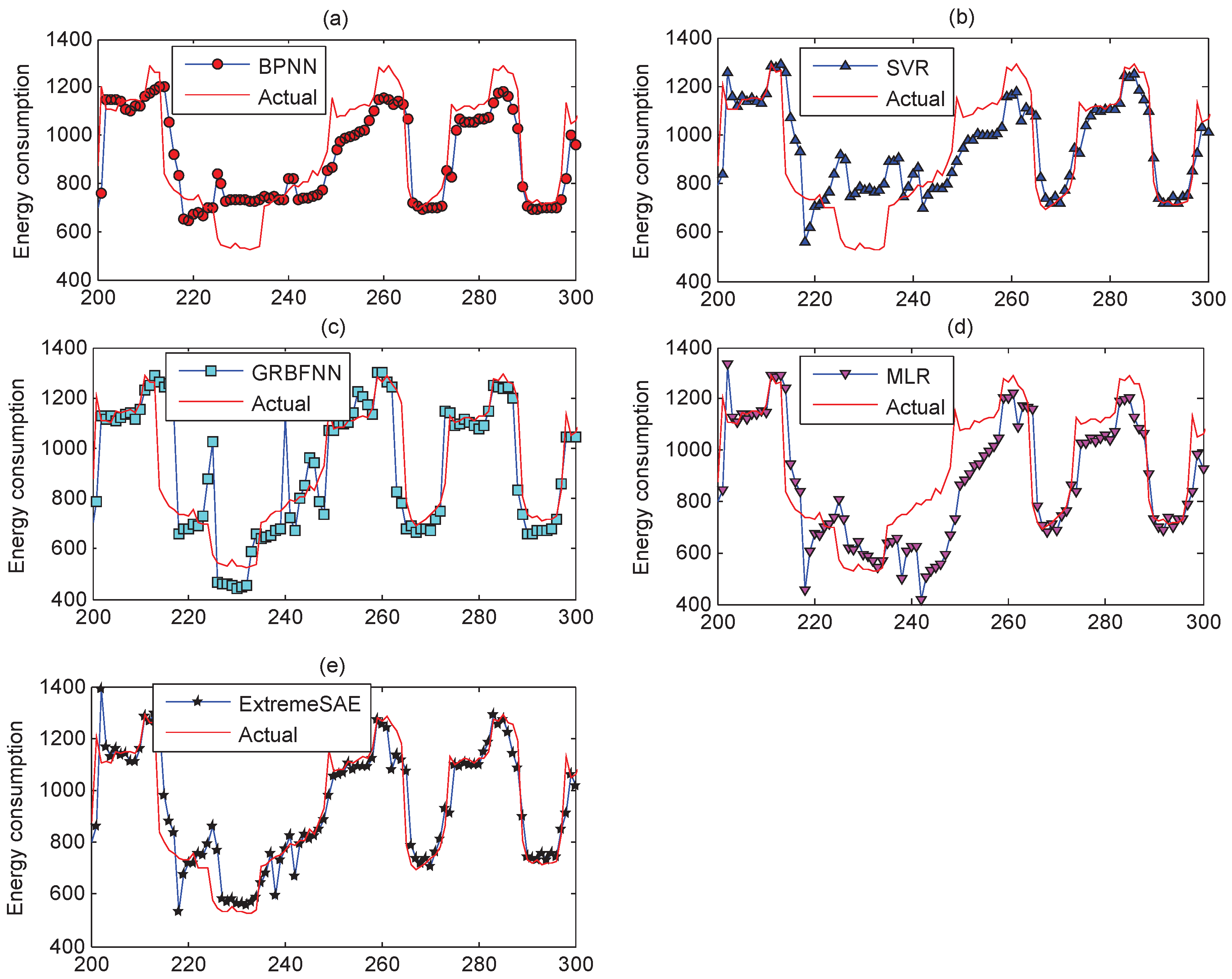
For the testing data, the prediction results of the five prediction models in the 60 min prediction experiment are demonstrated in Figure 11. Again, for better visualization, parts of the results (the values between 200 and 300) in Figure 11 have been zoomed in and are plotted in Figure 12 to demonstrate finer details.
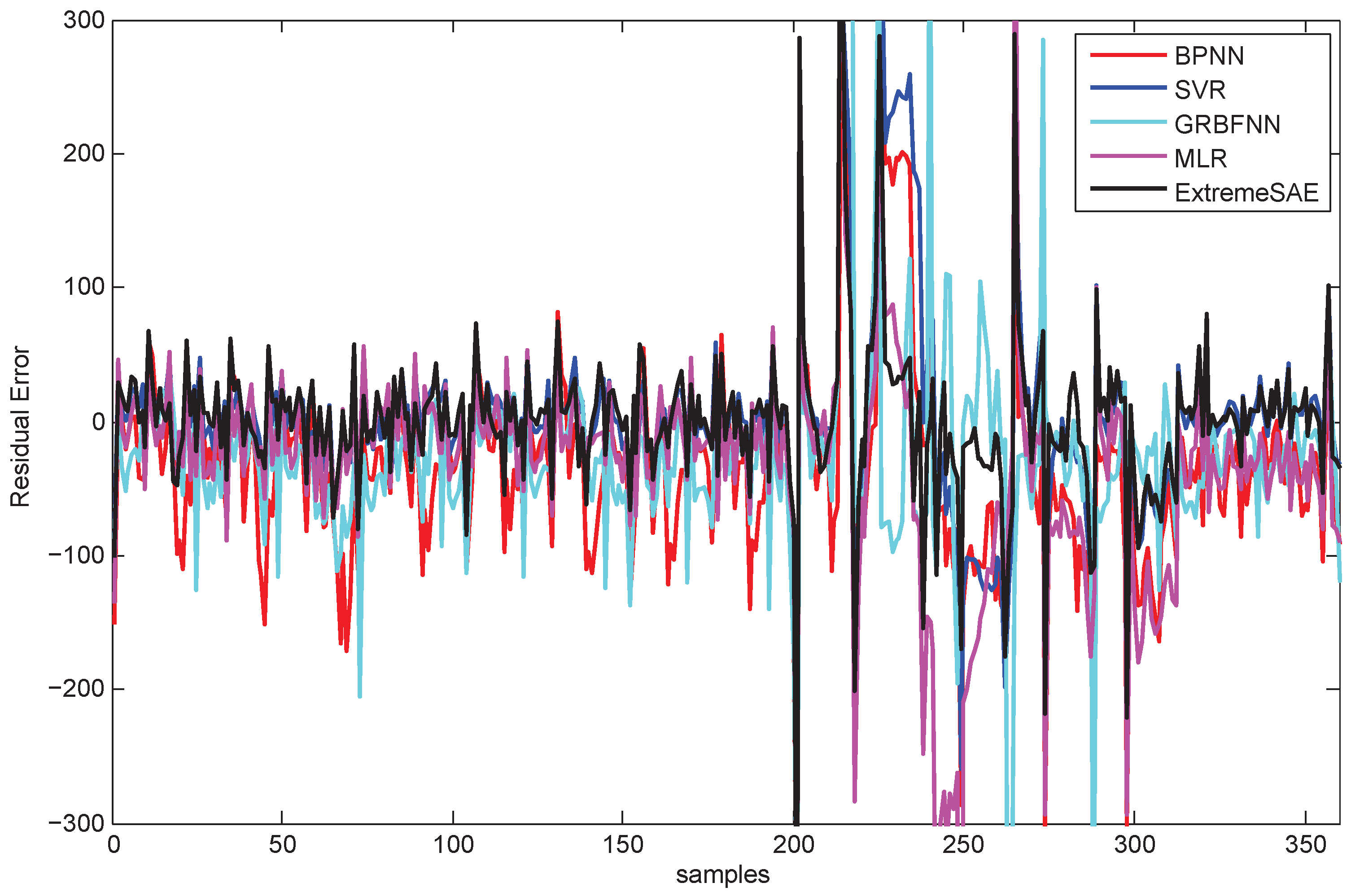
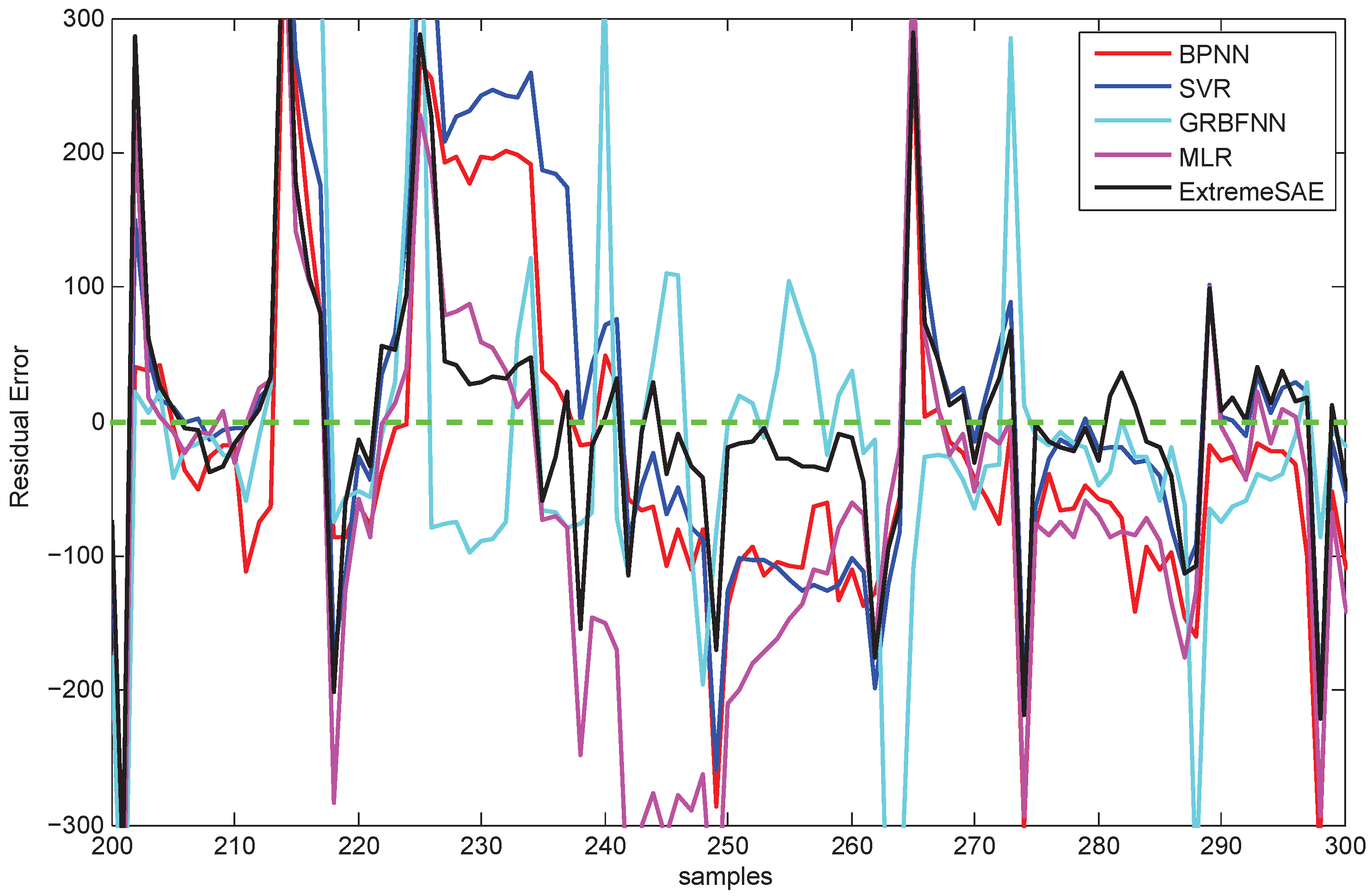
The residual errors of the five prediction models in the 60 min prediction experiment are demonstrated in Figure 13. Once more, parts of the results (the values between 200 and 300) in Figure 13 have been zoomed in and are re-plotted in Figure 14.
Similarly, in the 60 min prediction experiment, the MAEs, MREs and RMSEs of the five prediction models in the training and testing processes are listed in Table 4.
4.3. Comparisons and Discussion
Figure 6 and Figure 11 demonstrate the prediction performances of the five models for the testing data. From a global perspective, the proposed extreme SAE approach performs best, especially for the abnormal testing data that are from 400 to 500 in the 30 min experiment and from 200 to 250 in the 60 min experiment. These abnormal testing data reflect the uncertainties in the building energy consumption; that is to say, the proposed extreme SAE approach has the greatest ability to deal with the uncertain building energy consumption data. This judgement can also be observed and verified more clearly from Figure 7 and Figure 12.
Figure 8 and Figure 13 show the residual errors of the five models for the testing data. From both figures, we can observe that the residual errors of the extreme SAE usually lie in the smallest scale around zero compared with the four comparative methods. This phenomenon also indicates that the proposed deep learning approach has better prediction accuracy than the four comparative methods. The residual errors for the abnormal testing data, as shown in Figure 9 and Figure 14, reveal the performances of the five models in more detail. Again, the extreme SAE performs best. We can also observe that MLR has the poorest performance in both experiments. This also verifies that the artificial intelligence methods always perform better than the statistical methods.
As shown in Table 2 and Table 4, from the point of view of the testing performance, the proposed deep learning approach has the smallest prediction error and the best accuracy for building energy consumption prediction, and its accuracy is promising. For the testing data, in the 30 min prediction experiment, the performance of the extreme SAE was at least 18.2%, 21.1% and 15.3% better according to the three indices when compared with the other four methods, and, in the 60 min prediction experiment, the values for the same indices were respectively 12.7%, 13.5% and 23.5% better when compared with the four comparative models.
Although the GRBFNN has the best training indices, its performances for the testing data are poor, and the over-fitting phenomenon in the training process of the GRBFNN is observed. Generally, MLR has the poorest performances both for the training and testing data, followed by the BPNN. SVR performs better than the GRBFNN, the BPNN and MLR, but performs worse than the proposed extreme SAE approach. In summary, in both experiments, extreme SAE > SVR > GRBFNN > BPNN > MLR, where > indicates “performs better than”. These facts again verify the better feature extraction ability of the deep learning model in the prediction of building energy consumption.
5. Conclusions
Deep learning has shown its powerful learning and prediction abilities in the time series prediction applications. This study aimed to utilize one popular deep learning approach—the SAE method—to improve the predicted results of building energy consumptions. Theoretically, this study provided a novel learning method by combining the SAE method and the ELM method. The main difference between the proposed method and the traditional SAE method is that the proposed method does not need the fine-tuning of the whole network by the iterative back-propagation algorithm, but directly utilizes the ELM method to find the output weights without iterations. This can quicken the learning speed and strengthen the generalization performance. For the application aspect, the proposed deep learning method was applied to the energy consumption prediction of a specific building, whose one year energy consumption data were collected. The experimental and comparison results demonstrate that the deep learning method outperforms several popular traditional machine learning methods. The reason for this may be that the proposed deep learning method has deeper architecture and improved learning strategies compared with the other comparative methods. In other words, although the data set in this application does not have a large quantity of data, the deep learning method can still extract better building energy consumption features and improve the prediction accuracy.
We are continuing to investigate other schemes to further improve the prediction accuracy. By analyzing the collected building energy consumption data, we found that the building energy consumption changes periodically. By considering its periodicity, achieving better performance may be expected. Then, what is left to be investigated is how to simultaneously utilize both the data and the prior knowledge of periodicity to construct the DNN. This will be one of our future research directions.
Acknowledgments
This work is supported by the National Natural Science Foundation of China (61473176, 61105077, and 61573225), and the Natural Science Foundation of Shandong Province for Young Talents in Provincial Universities (ZR2015JL021).
Author Contributions
Chengdong Li, Dongbin Zhao and Jianqiang Yi have contributed to developing ideas about energy consumption prediction and collecting the data. Zixiang Ding and Guiqing Zhang programmed the algorithm and tested it. All the authors were involved in preparing the manuscript.
Conflicts of Interest
The authors declare no conflict of interest.
References
- Štreimikienė, S. Residential energy consumption trends, main drivers and policies in Lithuania. Renew. Sustain. Energy Rev. 2014, 35, 285–293. [Google Scholar] [CrossRef]
- Ugursal, V.I. Energy consumption, associated questions and some answers. Appl. Energy 2014, 130, 783–792. [Google Scholar] [CrossRef]
- Hua, C.; Lee, W.L.; Wang, X. Energy assessment of office buildings in China using China building energy codes and LEED 2.2. Energy Build. 2015, 86, 514–524. [Google Scholar]
- Zuo, J.; Zhao, Z.Y. Green building research-current status and future agenda: A review. Renew. Sustain. Energy Rev. 2014, 30, 271–281. [Google Scholar] [CrossRef]
- Daut, M.A.M.; Hassan, M.Y.; Abdullah, H.; Rahman, H.A.; Abdullah, M.P.; Hussin, F. Building electrical energy consumption forecasting analysis using conventional and artificial intelligence methods: A review. Renew. Sustain. Energy Rev. 2017, 70, 1108–1118. [Google Scholar] [CrossRef]
- Li, K.; Hu, C.; Liu, G.; Xue, W. Building’s electricity consumption prediction using optimized artificial neural networks and principal component analysis. Energy Build. 2015, 108, 106–113. [Google Scholar] [CrossRef]
- Pombeiro, H.; Santos, R.; Carreira, P.; Silva, C.; Sousa, J.M.C. Comparative assessment of low-complexity models to predict electricity consumption in an institutional building: Linear regression vs. fuzzy modeling vs. neural networks. Energy Build. 2017, 146, 141–151. [Google Scholar] [CrossRef]
- Jimenez, M.J.; Heras, M.R. Application of multi-output ARX models for estimation of the U and g values of building components in outdoor testing. Sol. Energy 2005, 79, 302–310. [Google Scholar] [CrossRef]
- Kimbara, A.; Kurosu, S.; Endo, R.; Kamimura, K.; Matsuba, T.; Yamada, A. On-line prediction for load profile of an air-conditioning system. Ashrae Trans. 1995, 101, 198–207. [Google Scholar]
- Newsham, G.R.; Birt, B.J. Building-level occupancy data to improve ARIMA-based electricity use forecasts. In Proceedings of the 2nd ACM Workshop on Embedded Sensing Systems for Energy-Efficiency in Building, Zurich, Switzerland, 2 November 2010; pp. 13–18. [Google Scholar]
- Aydinalp-Koksal, M.; Ugursal, V.I. Comparison of neural network, conditional demand analysis, and engineering approaches for modeling end-use energy consumption in the residential sector. Appl. Energy 2008, 85, 271–296. [Google Scholar] [CrossRef]
- Hsu, D. Comparison of integrated clustering methods for accurate and stable prediction of building energy consumption data. Appl. Energy 2015, 160, 153–163. [Google Scholar] [CrossRef]
- Alvarez, F.M.; Troncoso, A.; Riquelme, J.C.; Ruiz, J.S.A. Energy time series forecasting based on pattern sequence similarity. IEEE Trans. Knowl. Data Eng. 2011, 23, 1230–1243. [Google Scholar] [CrossRef]
- Pérez-Chacón, R.; Talavera-Llames, R.L.; Martinez-Alvarez, F.; Troncoso, A. Finding electric energy consumption patterns in big time series data. In Proceedings of the13th International Conference Distributed Computing and Artificial Intelligence, Sevilla, Spain, 1–3 June 2016; Springer: Cham, Switzerland, 2016; pp. 231–238. [Google Scholar]
- Martínez-Álvarez, F.; Troncoso, A.; Asencio-Cortés, G.; Riquelme, J.C. A survey on data mining techniques applied to electricity-related time series forecasting. Energies 2015, 8, 13162–13193. [Google Scholar] [CrossRef]
- Tso, G.K.F.; Yau, K.K.W. Predicting electricity energy consumption: A comparison of regression analysis, decision tree and neural networks. Energy 2007, 32, 1761–1768. [Google Scholar] [CrossRef]
- Ahmad, M.W.; Mourshed, M.; Rezgui, Y. Trees vs. Neurons: Comparison between random forest and ANN for high-resolution prediction of building energy consumption. Energy Build. 2017, 147, 77–89. [Google Scholar] [CrossRef]
- Paudel, S.; Elmitri, M.; Couturier, S.; Nguyen, P.H.; Kamphuis, R.; Lacarrière, B.; Corre, O.L. A relevant data selection method for energy consumption prediction of low energy building based on support vector machine. Energy Build. 2017, 138, 240–256. [Google Scholar] [CrossRef]
- Mena, R.; Rodríguez, F.; Castilla, M.; Arahal, M.R. A prediction model based on neural networks for the energy consumption of a bioclimatic building. Energy Build. 2014, 82, 142–155. [Google Scholar] [CrossRef]
- Biswas, M.A.R.; Robinson, M.D.; Fumo, N. Prediction of residential building energy consumption: A neural network approach. Energy 2016, 117, 84–92. [Google Scholar] [CrossRef]
- Naji, S.; Shamshirband, S.; Basser, H.; Keivani, A.; Alengaram, U.J.; Jumaat, M.Z.; Petkovic, D. Application of adaptive neuro-fuzzy methodology for estimating building energy consumption. Renew. Sustain. Energy Rev. 2016, 53, 1520–1528. [Google Scholar] [CrossRef]
- Ekici, B.B.; Aksoy, U.T. Prediction of building energy needs in early stage of design by using ANFIS. Expert Syst. Appl. 2011, 38, 5352–5358. [Google Scholar] [CrossRef]
- Yang, J.; Rivard, H.; Zmeureanu, R. On-line building energy prediction using adaptive artificial neural networks. Energy Build. 2005, 37, 1250–1259. [Google Scholar] [CrossRef]
- Naji, S.; Keivani, A.; Shamshirband, S.; Alengaram, U.J.; Jumaat, M.Z.; Mansor, Z.; Lee, M. Estimating building energy consumption using extreme learning machine method. Energy 2016, 97, 506–516. [Google Scholar] [CrossRef]
- Zhang, Y.; Chen, Q. Prediction of building energy consumption based on PSO-RBF neural network. In Proceedings of the IEEE International Conference on System Science and Engineering, Shanghai, China, 11–13 July 2014; pp. 60–63. [Google Scholar]
- Hinton, G.E.; Osindero, S.; Teh, Y.W. A fast learning algorithm for deep belief nets. Neural Comput. 2014, 18, 1527–1554. [Google Scholar] [CrossRef] [PubMed]
- Collobert, R.; Weston, J. A unified architecture for natural language processing: Deep neural networks with multitask learning. In Proceedings of the 25th International Conference on Machine Learning, Helsinki, Finland, 5–9 July 2008; pp. 160–167. [Google Scholar]
- Hinton, G.E.; Salakhutdinov, R.R. Reducing the dimensionality of data with neural networks. Science 2006, 313, 504–507. [Google Scholar] [CrossRef] [PubMed]
- Huval, B.; Coates, A.; Ng, A. Deep learning for class-generic object detection. arXiv, 2013; arXiv:1312.6885. [Google Scholar]
- Qiu, X.; Zhang, L.; Ren, Y.; Suganthan, P.N.; Amaratunga, G. Ensemble deep learning for regression and time series forecasting. In Proceedings of the 2014 IEEE Symposium on Computational Intelligence in Ensemble Learning (CIEL), Orlando, FL, USA, 9–12 December 2014; pp. 1–6. [Google Scholar]
- Li, L.; Lv, Y.; Wang, F.Y. Traffic signal timing via deep reinforcement learning. IEEE/CAA J. Autom. Sin. 2016, 3, 247–254. [Google Scholar]
- Lv, Y.; Duan, Y.; Kang, W.; Li, Z.; Wang, F.Y. Traffic flow prediction with big data: A deep learning approach. IEEE Trans. Intell. Transp. Syst. 2015, 16, 865–873. [Google Scholar] [CrossRef]
- Torres, J.; Fernández, A.; Troncoso, A.; Martínez-Álvarez, F. Deep learning-based approach for time series forecasting with application to electricity load. In Proceedings of the International Work-Conference on the Interplay between Natural and Artificial Computation, Corunna, Spain, 19–23 June2017; Springer: Cham, Switzerland, 2017; pp. 203–212. [Google Scholar]
- Bengio, Y.; Lamblin, P.; Dan, P.; Larochelle, H. Greedy layer-wise training of deep networks. In Proceedings of the International Conference on Neural Information Processing Systems, Vancouver, BC, Canada, 4–7 December 2006; pp. 153–160. [Google Scholar]
- Vincent, P.; Larochelle, H.; Bengio, Y.; Manzagol, P.A. Extracting and composing robust features with denoising autoencoders. In Proceedings of the 25th International Conference on Machine Learning, Helsinki, Finland, 5–9 July 2008; ACM: New York, NY, USA, 2008; pp. 1096–1103. [Google Scholar]
- Palm, R.B. Prediction as a Candidate for Learning Deep Hierarchical Models of Data; Technical University of Denmark: Kongens Lyngby, Denmark, 2012; Volume 5. [Google Scholar]
- Hosseiniasl, E.; Zurada, J.M.; Nasraoui, O. Deep learning of part-based representation of data using sparse autoencoders with nonnegativity constraints. IEEE Trans. Neural Netw. Learn. Syst. 2016, 27, 2486–2498. [Google Scholar] [CrossRef] [PubMed]
- Xu, J.; Xiang, L.; Liu, Q.; Gilmore, H.; Wu, J.; Tang, J.; Madabhushi, A. Stacked sparse autoencoder (SSAE) for nuclei detection on breast cancer histopathology images. IEEE Trans. Med. Imaging 2016, 35, 119–130. [Google Scholar] [CrossRef] [PubMed]
- Tao, C.; Pan, H.; Li, Y.; Zou, Z. Unsupervised spectral-spatial feature learning with stacked sparse autoencoder for hyperspectral imagery classification. IEEE Geosci. Remote Sens. Lett. 2015, 12, 2438–2442. [Google Scholar]
- Erhan, D.; Bengio, Y.; Courville, A.; Manzagol, P.A.; Vincent, P.; Bengio, S. Why does unsupervised pre-training help deep learning? J. Mach. Learn. Res. 2010, 11, 625–660. [Google Scholar]
- Huang, G.B.; Wang, D.H.; Lan, Y. Extreme learning machines: A survey. Int. J. Mach. Learn. Cybern. 2011, 2, 107–122. [Google Scholar] [CrossRef]
- Huang, G.B.; Zhu, Q.Y.; Siew, C.K. Extreme learning machine: Theory and applications. Neurocomputing 2006, 70, 489–501. [Google Scholar] [CrossRef]
- Li, M.B.; Huang, G.B.; Saratchandran, P.; Sundararajan, N. Letters: Fully complex extreme learning machine. Neurocomputing 2005, 68, 306–314. [Google Scholar] [CrossRef]
- Erb, R.J. Introduction to backpropagation neural network computation. Pharm. Res. 1993, 10, 165–170. [Google Scholar] [CrossRef] [PubMed]
- Awad, M.; Khanna, R. Support vector regression. Neural Inf. Process. Lett. Rev. 2007, 11, 203–224. [Google Scholar]
- Friedrichs, F.; Schmitt, M. On the power of Boolean computations in generalized RBF neural networks. Neurocomputing 2005, 63, 483–498. [Google Scholar] [CrossRef]
- Preacher, K.J.; Curran, P.J.; Bauer, D.J. Computational tools for probing interactions in multiple linear regression, multilevel modeling, and latent curve analysis. J. Educ. Behav. Stat. 2006, 31, 437–448. [Google Scholar] [CrossRef]
- Eberly, L.E. Multiple linear regression. Methods Mol. Biol. 2007, 404, 165–187. [Google Scholar] [PubMed]
- Chong, T.L. Estimating the differencing parameter via the partial autocorrelation function. J. Econom. 1998, 97, 365–381. [Google Scholar] [CrossRef]
- Zhang, Z.; Law, C.L.; Gunawan, E. Multipath mitigation technique based on partial autocorrelation function. Wirel. Pers. Commun. 2007, 41, 145–154. [Google Scholar] [CrossRef]
- Alder, B.J.; Wainwright, T.E. Decay of the Velocity Autocorrelation Function. Phys. Rev. A 1970, 1, 18–21. [Google Scholar] [CrossRef]
- Jiang, X.; Adeli, H. Wavelet Packet-Autocorrelation Function Method for Traffic Flow Pattern Analysis. Comput. Aided Civ. Infrastruct. Eng. 2010, 19, 324–337. [Google Scholar] [CrossRef]
Figure 1.
The autoencoder.

Figure 2.
The stacked autoencoders with k hidden layers and its layerwise training process.

Figure 3.
The structure of the extreme SAE with k hidden layers.

Figure 4.
The first 500 samples of the 30 and 60 min experiments.

Figure 5.
The partial autocorrelation function (PACF) of the 30 min experiment with 150 time lags.

Figure 6.
Prediction results of the five models in the 30 min experiment.

Figure 7.
Parts of the zoomed-in prediction results: (a) backward propagation neural network (BPNN); (b) support vector regression (SVR); (c) generalized radial basis function neural network (GRBFNN); (d) multiple linear regression (MLR); and (e) extreme stacked autoencoder (SAE).
Figure 7.
Parts of the zoomed-in prediction results: (a) backward propagation neural network (BPNN); (b) support vector regression (SVR); (c) generalized radial basis function neural network (GRBFNN); (d) multiple linear regression (MLR); and (e) extreme stacked autoencoder (SAE).

Figure 8.
Residual errors of the five models in the 30 min prediction experiment.

Figure 9.
Parts of the zoomed-in residual errors.

Figure 10.
The partial autocorrelation function (PACF) of the 60-min prediction experiment with 80 lags.
Figure 10.
The partial autocorrelation function (PACF) of the 60-min prediction experiment with 80 lags.

Figure 11.
Prediction results of the five models in the 60 min experiment.

Figure 12.
Parts of the zoomed-in prediction results: (a) backward propagation neural network (BPNN); (b) support vector regression (SVR); (c) generalized radial basis function neural network (GRBFNN); (d) multiple linear regression (MLR); and (e) extreme stacked autoencoder (SAE).
Figure 12.
Parts of the zoomed-in prediction results: (a) backward propagation neural network (BPNN); (b) support vector regression (SVR); (c) generalized radial basis function neural network (GRBFNN); (d) multiple linear regression (MLR); and (e) extreme stacked autoencoder (SAE).

Figure 13.
Residual errors of the five models in the 60 min prediction experiment.

Figure 14.
Parts of the zoomed-in residual errors.


Table 1.
Root-mean-square errors (RMSEs) of the 30 min experiment with various numbers of hidden layers and hidden units.
Table 1.
Root-mean-square errors (RMSEs) of the 30 min experiment with various numbers of hidden layers and hidden units.
| 23.4814 | 23.5453 | 23.4509 | 23.1802 | |
| 22.9833 | 23.5639 | 23.3679 | 22.9015 | |
| 24.3893 | 24.2911 | 24.3733 | 24.6273 | |
| 23.9358 | 24.3908 | 24.5166 | 24.2795 | |
| 23.3932 | 24.2846 | 23.8729 | 24.0003 | |
| 24.0451 | 24.2820 | 24.4101 | 24.2295 | |
| 23.9541 | 23.8668 | 23.4668 | 23.9033 | |
| 23.3656 | 23.6728 | 23.5747 | 23.7575 |
Table 2.
Comparison results of the five prediction models in the 30 min prediction experiment.
| Performance | Training | Testing | |||||
|---|---|---|---|---|---|---|---|
| Methods | MAE | MRE (%) | RMSE | MAE | MRE (%) | RMSE | |
| Extreme SAE | 15.0231 | 3.0082 | 23.3090 | 13.3865 | 2.9174 | 22.9015 | |
| BPNN | 26.5890 | 4.9600 | 35.4052 | 21.3020 | 4.1792 | 30.8121 | |
| SVR | 15.8168 | 3.1991 | 25.3225 | 16.3592 | 3.6917 | 27.0380 | |
| GRBFNN | 11.7406 | 2.3532 | 17.7543 | 18.0785 | 3.8928 | 34.2312 | |
| MLR | 31.3272 | 6.4854 | 40.6747 | 25.7448 | 5.4652 | 38.8463 | |
Table 3.
Root-mean-square errors (RMSEs) of the 60 min prediction experiment with various numbers of hidden layers and hidden units.
Table 3.
Root-mean-square errors (RMSEs) of the 60 min prediction experiment with various numbers of hidden layers and hidden units.
| 59.4885 | 59.1812 | 59.8399 | 59.2147 | |
| 63.3515 | 63.4566 | 63.5216 | 63.1455 | |
| 62.3616 | 62.4175 | 62.9833 | 63.5690 | |
| 64.6232 | 64.9396 | 65.4826 | 68.3591 | |
| 63.9450 | 63.5129 | 64.6592 | 63.9566 | |
| 65.6216 | 64.4153 | 64.1315 | 64.5682 | |
| 66.2908 | 64.9708 | 66.1777 | 65.6557 | |
| 66.3097 | 64.3294 | 66.2774 | 66.3823 |
Table 4.
Comparison results of the five prediction models in the 60 min prediction experiment.
| Performance | Training | Testing | |||||
|---|---|---|---|---|---|---|---|
| Methods | MAE | MRE (%) | RMSE | MAE | MRE (%) | RMSE | |
| Extreme SAE | 32.1336 | 3.2429 | 54.3246 | 33.7168 | 3.6420 | 59.1812 | |
| BPNN | 65.0351 | 6.0898 | 85.4008 | 59.2456 | 6.3922 | 84.9968 | |
| SVR | 34.3843 | 3.5179 | 58.6403 | 43.4038 | 5.1010 | 77.3101 | |
| GRBFNN | 23.6996 | 2.3306 | 38.6174 | 38.6145 | 4.2105 | 80.7410 | |
| MLR | 63.9774 | 6.6008 | 85.2207 | 56.0647 | 5.9556 | 89.9583 | |
© 2017 by the authors. Licensee MDPI, Basel, Switzerland. This article is an open access article distributed under the terms and conditions of the Creative Commons Attribution (CC BY) license (http://creativecommons.org/licenses/by/4.0/).
Share and Cite
MDPI and ACS Style
Li, C.; Ding, Z.; Zhao, D.; Yi, J.; Zhang, G. Building Energy Consumption Prediction: An Extreme Deep Learning Approach. Energies 2017, 10, 1525. https://doi.org/10.3390/en10101525
AMA Style
Li C, Ding Z, Zhao D, Yi J, Zhang G. Building Energy Consumption Prediction: An Extreme Deep Learning Approach. Energies. 2017; 10(10):1525. https://doi.org/10.3390/en10101525
Chicago/Turabian StyleLi, Chengdong, Zixiang Ding, Dongbin Zhao, Jianqiang Yi, and Guiqing Zhang. 2017. "Building Energy Consumption Prediction: An Extreme Deep Learning Approach" Energies 10, no. 10: 1525. https://doi.org/10.3390/en10101525
Note that from the first issue of 2016, this journal uses article numbers instead of page numbers. See further details here.