Energy Consumption Forecasting for University Sector Buildings
by
Khuram Pervez Amber
1,*, 
Muhammad Waqar Aslam
2,
Anzar Mahmood
3,
Anila Kousar
3,
Muhammad Yamin Younis
1,
Bilal Akbar
1,
Ghulam Qadar Chaudhary
1 and
Syed Kashif Hussain
1 1
Department of Mechanical Engineering, Mirpur University of Science and Technology (MUST), Mirpur 10250 (AJK), Pakistan
2
Department of Computer System Engineering, Mirpur University of Science and Technology (MUST), Mirpur 10250 (AJK), Pakistan
3
Department of Electrical (Power) Engineering, Mirpur University of Science and Technology (MUST), Mirpur 10250 (AJK), Pakistan
*
Author to whom correspondence should be addressed.
Energies 2017, 10(10), 1579; https://doi.org/10.3390/en10101579
Submission received: 22 August 2017
/
Revised: 29 September 2017
/
Accepted: 10 October 2017
/
Published: 12 October 2017
(This article belongs to the Special Issue Selected Papers from SEEP2017: The 10th International Conference on Sustainable Energy and Environmental Protection)
Abstract
:Reliable energy forecasting helps managers to prepare future budgets for their buildings. Therefore, a simple, easier, less time consuming and reliable forecasting model which could be used for different types of buildings is desired. In this paper, we have presented a forecasting model based on five years of real data sets for one dependent variable (the daily electricity consumption) and six explanatory variables (ambient temperature, solar radiation, relative humidity, wind speed, weekday index and building type). A single mathematical equation for forecasting daily electricity usage of university buildings has been developed using the Multiple Regression (MR) technique. Data of two such buildings, located at the Southwark Campus of London South Bank University in London, have been used for this study. The predicted test results of MR model are examined and judged against real electricity consumption data of both buildings for year 2011. The results demonstrate that out of six explanatory variables, three variables; surrounding temperature, weekday index and building type have significant influence on buildings energy consumption. The results of this model are associated with a Normalized Root Mean Square Error (NRMSE) of 12% for the administrative building and 13% for the academic building. Finally, some limitations of this study have also been discussed.
1. Introduction
In the U.K., buildings are the major energy consuming sector, with a share of 40% [1]. The electricity consumption in Higher Education (HE) buildings is the major factor in the sector’s carbon emissions [2]. Energy management systems have gained rapid recognition in the U.K. HE sector after the Higher Education Funding Council of England (HEFCE) imposed a 43% reduction in carbon emissions by 2020 against the baseline year 2005 for its all member universities [3]. All member universities in England now have a dedicated energy management team consistently working to achieve this goal. Variation in the sector’s CO2 emissions for the period 2008/09 to 2014/2015 has been shown in Figure 1. It depicts that electricity consumption emerges as the major contributor with a share of 63%, next to which is natural gas with a share of 33.3% [1,4,5]. It can also be observed that annual reduction in sector’s emission is slow at a rate of 2.17% per year. During these five years (i.e., 2008/09 to 2014/15), the sector has been able to reduce its total carbon emissions only by 8%.
Table 1 presents variation in number of students, electricity and gas consumption, emissions and Gross Internal Area (GIA) for the English HE sector. Variation in the sector’s CO2 emissions with respect to GIA (m2) and number of students was reported in [4]. It was observed that sector’s emissions based on GIA decreased by 15.83% at an annual rate of 4.2% during 2008/09 to 2014/15; a promising result compared to total absolute CO2 emissions. Average CO2 emissions per square meter area of a typical university campus in England were reported to be 90 kg/m2 for this period. The average CO2 emissions per student during the same period were 1210 kg/student. In this context, the CO2 emissions decreased by 7.8% during 2008/09 to 2014/15 with an annual decreasing rate of 1.86%.
Figure 2 presents variation in electricity consumption of the English HE sector for the period 2008/09 to 2014/15. It is evident from Figure 2 that sector’s total electricity consumption has been increasing since 2008/09 to 2014/15 at average annual rate of 1.87%. However, it could also be observed that due to energy efficiency initiatives of universities and injection of electricity from on-site Combined Heat and Power (CHP) plants as well as renewable sources (solar and wind) grid electricity consumption has decreased annually at 1.56%, totaling 6.27% lower in 2014/15 compared to 2008/09 levels. As grid electricity has higher carbon factor than the CHP or renewable electricity, therefore the decreased grid share corresponds to a higher decrease in carbon emissions.
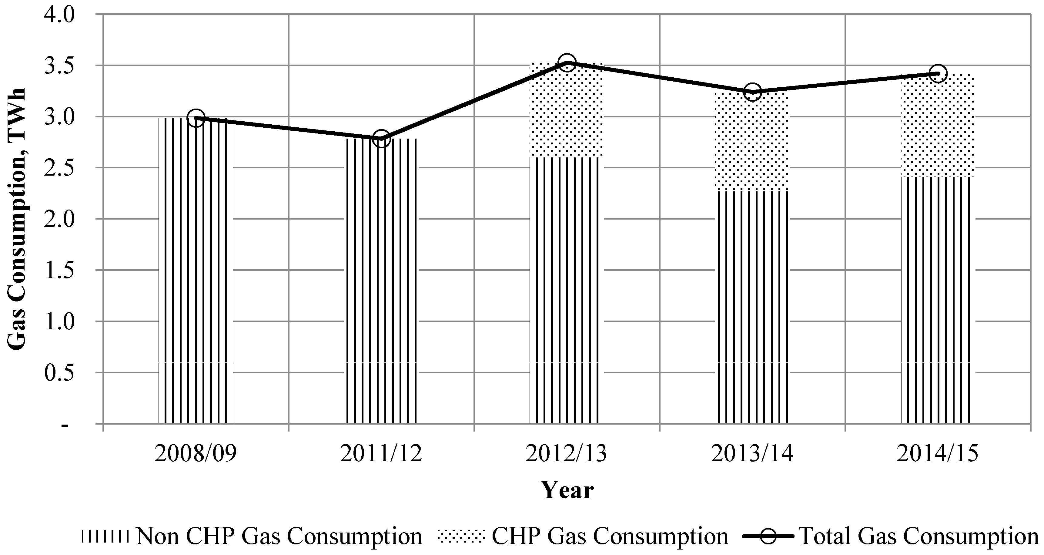
Annual variation of sector’s gas consumption is presented in Figure 3. Gas consumption was observed 14.5% higher in 2014/15 compared to 2008/09. This increase is associated with installations of CHP plants in universities for onsite energy generation. Towards the end of 2011–2012, 59 of the 161 U.K. universities had installed CHP on their campuses [3].
The overall effect of electricity and gas consumption could be judged by looking at the sector’s CO2 emission levels, which clearly shows that emissions are decreasing at a slower annual rate. This declining trend in carbon emissions certainly reflects the overall efforts made by the universities aiming to achieve their carbon-emissions reduction targets. However, despite such efforts and a number of ambitious initiatives, the English universities are far behind achieving their 2020 emissions reduction targets [6].
Energy consumption in university buildings is mainly driven by various factors such as; building type, building age, occupancy, operating hours, type of equipment installed and weather conditions. Nearly 68% space of a typical university campus in England is occupied by two major building categories, i.e., academic (42%) and administrative (26%) buildings [6]. In 2014/15, non-residential buildings of English universities consumed about 80% of total energy consumption where as 20% electricity consumption occurred in the sector’s residential buildings [4].
The aforementioned information clearly shows that electricity and gas consumption are the two major carbon emitting sources of the HE sector of England, with shares of 63% and 33%, respectively [4]. The sector’s slow declining trend of carbon emissions clearly indicates that the universities need to explore additional energy saving opportunities along with improving the energy management systems of the universities.
Monitoring and analyzing buildings energy consumption patterns is one of the major components of an effective energy management system which helps in understanding the building’s operational behavior under different conditions. It also helps in identifying undesired wastage of energy under specific conditions. If the energy consumption data are collected and maintained properly, their relation with different variables such as surrounding temperature, humidity, occupancy etc. could be investigated and future energy predictions could be made by taking these factors into account. Another key benefit is that predicted energy consumption data could be used to predict reliable energy budgets for future. Energy management teams of universities are responsible for monitoring, analyzing and maintaining energy consumption data of their buildings. They are responsible for preparing reliable energy consumption forecasts in order to prepare their energy budget forecasts for the coming years as well as identifying opportunities of energy conservation.
Reliable energy consumption forecasting plays a critical role in successful implementation of energy management systems. Many organizations have failed in managing energy consumption and budgeting because of lack of forecasting and use of less efficient forecasting techniques for planning [7,8]. Forecasting helps in evaluating the current and future economic conditions to steer the organization’s policies and decision making. It is a technique that predicts the future information based on historical and current information. A reliable forecasting can help universities financial and energy management teams to set up their priorities and strategic goals and it can act as an integral part of the annual budgeting process [9].
Different forecasting techniques such as Multiple Regression (MR), Artificial Neural Networks (ANN), and Genetic Algorithms (GA) have been widely used by researchers for energy consumption forecasting for different types of buildings in different regions [10]. Among these, MR is a simple, reliable and a quick technique [11,12,13,14]. A number of researchers [11,12,15,16,17,18,19,20,21,22,23,24] have used the MR method in their studies, but all such MR models forecast energy consumption of a single building or a region and require a lot of input data. Energy managers and their teams have always busy schedule and they would prefer a reliable and quick single model for different building categories instead of different forecasting models [24].
This research aims to facilitate the energy management teams of English universities by providing a simple, easy to use, quick and robust energy consumption forecasting model using MR technique in the form of a simple mathematical equation. Using this single equation, energy managers will be able to predict daily, monthly and yearly energy consumption of two different types of buildings, i.e., administrative and academic. For this purpose, two campus buildings (one academic and second administrative type) located in Southwark campus of London South Bank University (LSBU) are selected and their historical electricity consumption data are used in the development of forecasting model. Daily electricity consumption data of these two buildings for a long period (i.e., 2007–2010) was available but daily gas consumption data was not available. Therefore, due to unavailability of daily gas consumption data, this research only focuses on electricity consumption forecasting model.
London South Bank University (LSBU) is a public university located in Central London. It has 17,735 students and 1700 staff and is based in the London Borough of Southwark. LSBU is located at 51.4982° N, 0.1021° W. The University has 31 buildings (GIA: 148,771 m2) in total, of which 19 are non-residential buildings occupying a Gross Internal Area (GIA) of 114,065 m2 while remaining 12 are residential buildings occupying GIA of 37,706 m2. The energy management team is responsible for energy and environment related matters such as:
- (a)
- Monitoring, analyzing and maintaining record of energy consumption;
- (b)
- Identifying energy reduction opportunities and setting up targets;
- (c)
- Compliance of national legislation/schemes such as Carbon Reduction Scheme (CRC);
- (d)
- Preparing forecasts for energy budgets based on historical energy consumption data;
- (e)
- Display Energy Certificates (DECs).
LSBU has to meet a target of 43% reduction in its CO2 emissions by 2020 against the base year 2005/06. In 2005/06, total emissions of LSBU were 12,165 tCO2 which means that it has to reduce its emissions to a level of 7907 tCO2 by 2020. Figure 4 shows variation in the CO2 emissions of LSBU for years 2008/09 to 2014/15. It is evident that due to University’s imperative energy reduction initiatives, the University has been able to reduce its CO2 emissions by 32% in 2014/15 compared to 2005/06. Major drop in CO2 emissions was observed between 2005/06 and 2008/09 where emissions dropped by 24%. However, from 2008/09 to 2014/15, LSBU was able to reduce its CO2 emissions just by 8%. Major sources of these CO2 emissions in LSBU are electricity (74%) and natural gas (26%).
The following researchers have applied MR method in their energy forecasting studies:
Fumo and Biswas [10] employed the MR method using long term hourly and daily energy consumption data of a domestic building. They used two explanatory variables, i.e., global irradiance and the outdoor temperature; the inclusion of former improved the coefficient of determination, R2, however, resulted in an increased RMSE.
Catlina et al. [12] used the MR method to predict heating energy consumption of buildings based on three factors namely; the building global heat loss coefficient, the south equivalent surface and the difference between the indoor set point temperature and the sol-air temperature (sol-air temperature (Tsol-air) is a variable used to calculate heating or cooling load of a building and determines the total heat gain through exterior surfaces.), that influence a building heat consumption. A detailed error analysis showed that their model presents a very good accuracy with R2 = 0.987.
Amiri et al. [22] developed two MR models for the prediction of annual cooling and heating energy consumptions of the buildings. Among the 17 tested explanatory variables 13 were found significant, of which occupancy schedule and exterior wall construction have major influence on cooling and heating loads. Both MR models were found good with R2 ranging from 0.95 to 0.98. Their study concluded that MR is an accurate, simple and fast way to obtain energy performance of administrative buildings.
Mastrucci et al. [23] employed the MR method to forecast electricity and natural gas consumption of domestic buildings in The Netherlands. In this study, the influence of type of dwelling, building age, floor area, and occupancy on the buildings natural gas and electricity consumption is analyzed. To assess the predictive power of the model, they used R2 and Mean Square Error (MSE). R2 values for natural gas and electricity models were found to be 0.718 and 0.817, respectively.
Bruan et al. [11] applied an MR method to investigate effect of outdoor temperature and humidity on the buildings electricity and gas consumption. It was found that temperature has the highest influence on the buildings energy consumption with R2 = 0.92 for electricity consumption and R2 = 0.85 for gas consumption. The predictive power of MR model has been tested by analyzing the Normalized Mean Biased Error (NMBE) and Coefficient of CVRMSE. It was found that NMBE is −2.6% whereas CVRMSE was found to be just below 3.8%.
Capozzoli et al. [25] analyzed annual heating energy consumptions of eighty school buildings in the north of Italy and developed an MR model to estimate energy consumption of these schools. They used nine different influencing variables and tested the predictive power of their model based on Mean Absolute Percentage Error (MAPE). The results of this study suggested that the MR model is a decent model with R2 = 0.85 and MAPE of 15%.
In the light of the above discussion, it is clearly seen that most of the MR models developed for energy forecasting purposes are for the single building category, whereas the energy managers of a typical university campus are responsible for different building categories. This highlights the significance of a quick and robust forecasting model for different building categories. This study, for the first time proposes a unique MR model for multiple building categories based on five years real historical data. This will not only provide a quick forecasting tool but also a reliable mean of forecasting energy consumption for multiple building categories. Energy managers will be able to prepare reliable energy budgets for their procurement of their annual energy usage in order to assist the higher management in setting up their financial priorities. Rest of the paper is organized as follows: Section 2 describes the methodology of this work whereas in Section 3 results have been discussed. Conclusions are drawn in Section 4.
2. Methods
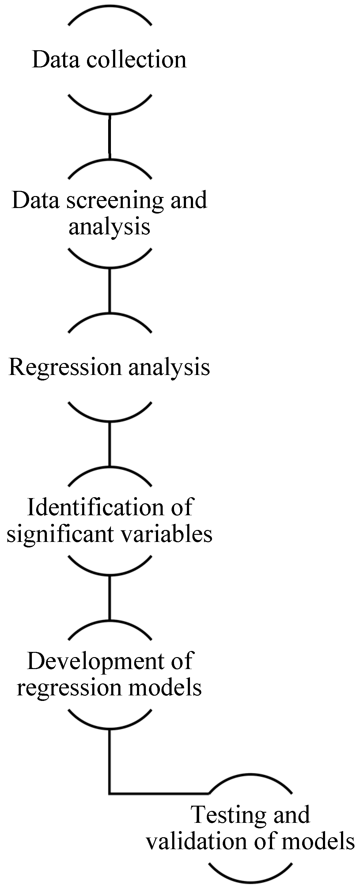
This section presents methods and details of different stages such as data collection, model development and its testing. Figure 5 shows all different stages which are illustrated in detail in the underlying sub-sections.
2.1. Data Collection
The following data for the explanatory and dependent variables for study period of five years January 2007–December 2011 have been used for this study:
- Dependent variable: Y = Daily electricity usage, Wh/m2;
- Explanatory variable 1: x1 = Daily mean surrounding temperature, K
- Explanatory variable 2: x2 = Daily mean global irradiance, W/m2
- Explanatory variable 3: x3 = Daily mean humidity, %
- Explanatory variable 4: x4 = Daily mean wind velocity, m/s
Further two proxy variables the weekday index and the building type are used in order to get more reliable results. These two are important variables as explained later by results; weekday index not only relates to building occupancy but also indirectly shows usage of available facilities while building type directly affects the energy usage. These two proxy explanatory variables are:
- Explanatory variable 5: x5 = Weekday Index (proxy variable for weekday type)
- Explanatory variable 6: x6 = Building Type (proxy variable for building type)
In addition to these variables, some information regarding both buildings such as operating hours, installed equipment etc. is also needed to elucidate their respective energy consumption patterns. Section 2.2 describes the different datasets, data sources, and methods of data collection.
2.2. Data Analysis
2.2.1. Buildings Description
All the relevant information of both buildings (academic and administrative) such as building area, operating hours, built year etc. is presented in Table 2.
Building age, its orientation, operating hours and type of installed equipment are very important variables having major impact on the buildings energy consumption. However, being identical, effect of these variables on energy consumption of both the buildings has not been investigated in this study.
2.2.2. Electricity Consumption Data
Daily electricity consumption (kWh) data for both buildings have been collected from the Energy Manager Office for the study period, and presented as consumption per unit area (Wh/m2) for each building.
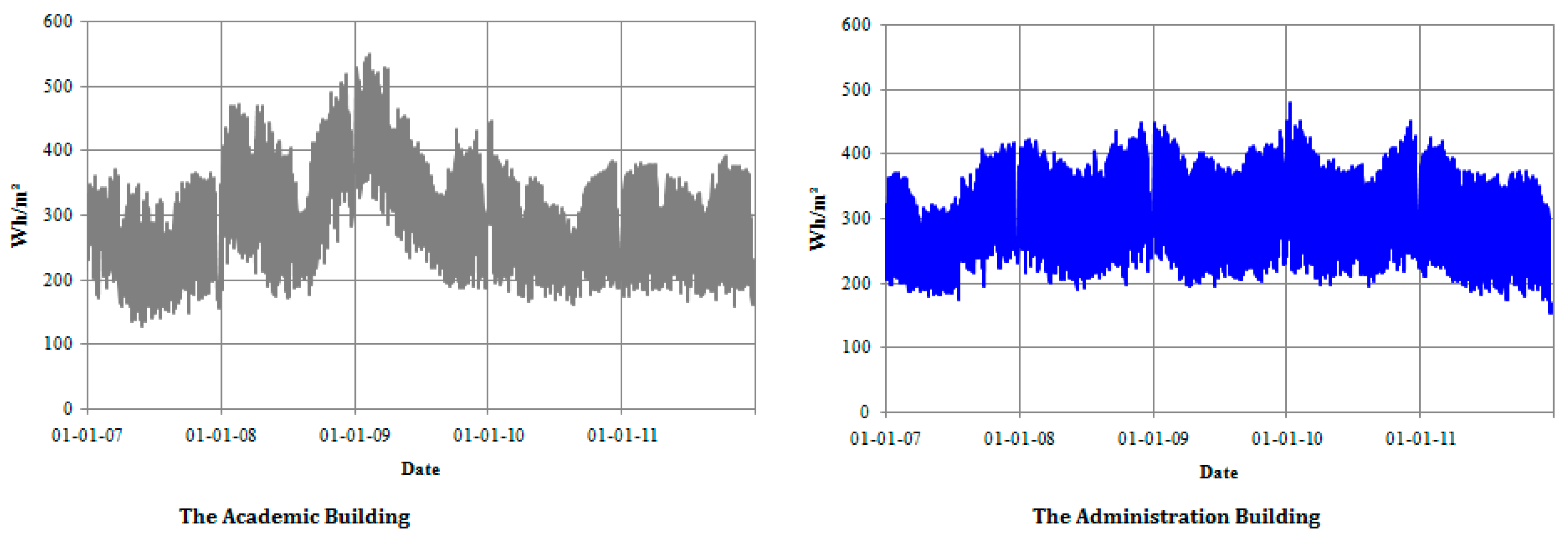
Figure 6 presents deviation in daily electricity usage of both academic and administrative buildings over the period 1 January 2007 to 31 December 2011 whereas Table 3 shows the stats of electricity consumption for non-working days (NWD) and working days (WD) for the two buildings.
- (a)
- The electricity consumption patterns of both buildings are nearly identical in shape and show drops during summer which are mainly due to low heating demand during summer and vice versa for winter. This indirectly refers to electricity consumption in the heating equipment such as pumps, boilers, air handling units, etc.
- (b)
- The consumption patterns (low in summer and high in winter) further suggest that surrounding temperature has a noteworthy effect on daily electricity usage of buildings. As both buildings under investigation are naturally ventilated (i.e., there is no cooling demand during summer), therefore, only seasonal load is heating during winter. During summer, heating plant and its accessories such as supply and return pumps, booster pumps, air handling units etc. are switched off, thus, electricity consumption drops to the base load. Other factors such as occupancy has limited effect as it remains somewhat constant throughout the year.
- (c)
- Electricity usage in both buildings during non-working days is also considerably large, i.e., nearly 58% of that on a working day. This is probably due to the automatic Building Management System (BMS) which switches the equipment ON and OFF regardless of the type of day (i.e., WD or NWD). This necessitates the additional automation of building control systems in accordance with the number of persons present in the building in order to save the energy.
2.2.3. Weather Data
Fluctuating weather conditions play a crucial role in building energy consumption. A number of studies [7,27,28,29,30,31,32,33,34,35] have investigated the effect of weather changes on building energy consumption. Amber, et al. [6] investigated the effect of four weather variables, i.e., surrounding temperature, global irradiance, humidity and wind velocity on the electricity usage of different buildings. Among the four variables the surrounding temperature found to be the critical parameter which drives the building energy consumption. Bruan et al. [11] also found that among outdoor temperature and humidity the former plays dominant role in building energy consumption. On the other hand Al-Garni et al. [34], with variable occupant populations, found the relative humidity and global irradiance as the critical variables as main driving force for the building energy consumption.
In this study, daily mean values of surrounding temperature, global irradiance, wind velocity and humidity for the Central London region have been used [36]. Figure 7 shows the variation in daily mean values of these four weather variables for the study period whereas Table 4 presents the stats, i.e., minimum, maximum and median values for all these weather variables. It is evident from Figure 7 and Table 4 that daily mean surrounding temperature in the London region remained in the range of −1 °C to 28 °C whereas humidity remained in the range of 81% to 100%. Peak value for global irradiance was 307 W/m2 and for wind velocity it was 6 m/s. The patterns of weather variables as shown in Figure 7 clearly suggest that there is a linear relationship among global irradiance, surrounding temperature and humidity whereas relationship between surrounding temperature and wind velocity is not strong. This relationship, among above mentioned variables, has been further analyzed statistically using regression analysis and discussed in Section 2.4 and Section 4.
2.2.4. Building Occupancy Data
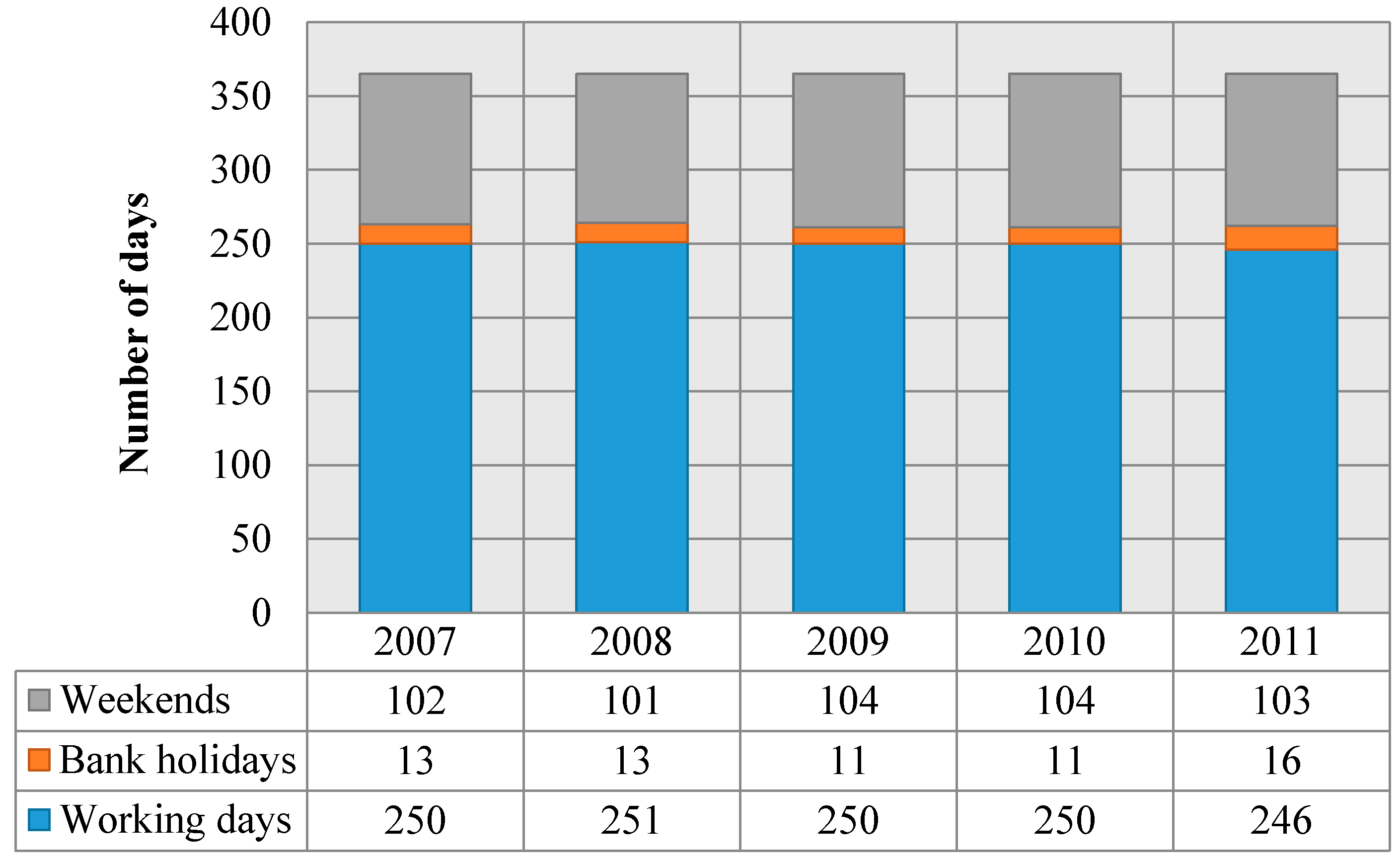
Another important variable that could significantly influence a building’s energy demand is its occupancy. Non-availability of the real occupancy data of the buildings under investigation is a limitation, so a proxy variable “weekday index” is therefore introduced to represent the building occupancy. Weekday index is used to distinguish the occupancy during the working and non-working days, a value of 1 for working days and 0 for non-working days (weekends and public holidays) is used. For this variable data of working and non-working days for years 2007 to 2011 is obtained from the U.K. bank calendar [37], and shown in Figure 8.
2.2.5. Building Type
Building type is another important factor that may influence the building energy consumption and therefore, its influence on the building electricity consumption must be investigated. Administrative building has been assigned a dummy value of 1 whereas academic building has a value of 2.
2.3. Data Normalization
Data normalization is a process to make the values of different variables lie within similar ranges. Sometimes the variables values lie within different dynamic ranges and the variables with higher values may have higher influence on the development of a model, although these variables may not necessarily be significant. In such a scenario, it becomes important to normalize the data so that the values of variables are within similar range. In this study, the variables have been normalized by using their respective mean and variance values [38]:
where is the ith value of kth variable, is the mean of kth variable, . is the standard deviation and is the normalized value of the variable. This is a linear normalization method and all the new values will now have zero mean and unit variance.
2.4. Regression Analysis
For forecasting daily electricity usage of both buildings, MR technique has been employed using SPSS software. MR is a statistical tool that helps to study how multiple explanatory variables are co-related to a dependent variable. Once this relationship among dependent and explanatory variables is identified, MR could be used for the prediction of dependent variable [11].
The multiple linear regression equation is as follows:
where:
- is the predicted or expected value of the dependent variable,
- through are distinct explanatory or predictor variables, where n represents a particular variable, d represents a particular day and t represents the building type,
- is the value of Y when all of the explanatory variables are equal to zero, and,
- through are the estimated regression coefficients. Each regression coefficient represents the change in “Y” relative to a unit change in the respective explanatory variable.
The predictive power of a MR model could be assessed by looking at its R2 value. R2 is a statistical measure of how close the data are to the fitted regression line. It is also known as the coefficient of multiple determination for multiple regression and it ranges from 0 to 1.
It is defined as:
where:
- Yobserved Real value of dependent variable,
- Ypredicted Predicted value of dependent variable,
- Yobserved, mean Mean of real values of dependent variable.
A value of R2 = 1 indicates that the fitted model explains all variations in Y, while R2 = 0 indicates no “linear” relationship between the dependent and explanatory variables [12]. An interior value such as R2 = 0.72 may be interpreted as follows: “Seventy two percent of the variance in the dependent variable can be explained by the explanatory variables. The remaining twenty eight percent can be attributed to unknown, lurking variables or inherent variability”.
One of the main checks in the MR model is the collinearity check, also known as multi-collinearity check among the explanatory variables as such situation can lead to ambiguous results that are associated with unstable estimated regression coefficients and affects the calculations associated to individual predictors [11,12]. Where one or more explanatory variables are collinear, one should be kept while others are dropped.
3. Results and Analysis
In this study, multiple regression method has been applied on the data for the period from 1 January 2007 to 31 December 2010 for identification of significant and insignificant variables. Table 5 gives the preliminary MR results and a collinearity analysis among various variables. The MR model suggests that all the variables except wind velocity have p-values less than 0.05 demonstrating that all the variables except wind velocity are significant and cannot be ignored [39]. Wind velocity having p-value higher than 0.05 indicates its weaker relationship with the buildings electricity consumption. The overall R2 value for all the variables is 0.73 which shows high relevance between the explanatory and the dependent variables. The collinearity analysis in Table 5 gives a picture of relevancy of variables among themselves. A high collinearity between any two variables suggests that only one of them can be used as they behave in a similar way. Table 5 demonstrates high collinearity (R = 0.69) between surrounding temperature and global irradiance. A similar trend is seen between global irradiance and relative humidity with a collinearity value −0.61 while surrounding temperature and relative humidity have relatively weak (−0.42) collinearity value. Since the surrounding temperature has a high collinearity with global irradiance and same is true for global irradiance and humidity. Therefore, the latter two variables (global irradiance and humidity) can be dropped and former (temperature) should be considered. Rest of the variables have poor collinearity with each other so these can also be included. Wind velocity being insignificant could be eliminated from further analysis. A final modified MR model is presented in Table 6. The model’s equation for predicting daily electricity usage (Wh/m2) of the administrative or academic building is given by Equation (4):
which implies that Ed = f (x1, x5, x6), where x1 = Daily mean normalized surrounding temperature; x5 = Normalized Weekday Index; x6 = Normalized Building type.
Ed = 323.62 − 21.87x1 + 67.49x5 − 6.37x6
The MR model equation clearly demonstrates that there is a negative linear relationship among daily electricity consumption and surrounding temperature. This is true as high temperature will reduce heating demand of the buildings which means heating equipment and its accessories such as pumps, air handling units (AHUs) etc. will not run thus resulting in decrease in daily electricity consumption. It also suggests that daily electricity consumption on a working day will exceed by 145.3 Wh/m2 than that on a non-working day.
The proposed model has R2 value of 0.72 (the preliminary model had 0.73), demonstrating that the predictive power of model has not changed much after dropping three variables. Therefore, from the R2 analysis, it is obvious that the proposed model is an effective predictive model. By putting the values of surrounding temperature, building type and weekday index, one could easily forecast daily electricity usage of their buildings and could prepare a reliable energy budget forecast. This model equation has been tested to predict electricity consumption of the same two buildings for the period 1 January 2011 to 31 December 2011. Later, this forecasted electricity consumption has been compared with real daily electricity consumption of the two buildings for the same period and it is discussed in next section.
4. Discussion
This section presents the model testing and its validation and finally discusses the error analysis. By inputting the real values of daily mean surrounding temperature, building type and weekday index in Equation (3) for the study period, daily electricity usage for both buildings have been forecasted. The predicted values of daily electricity usage were compared with the real daily electricity usage of both buildings.
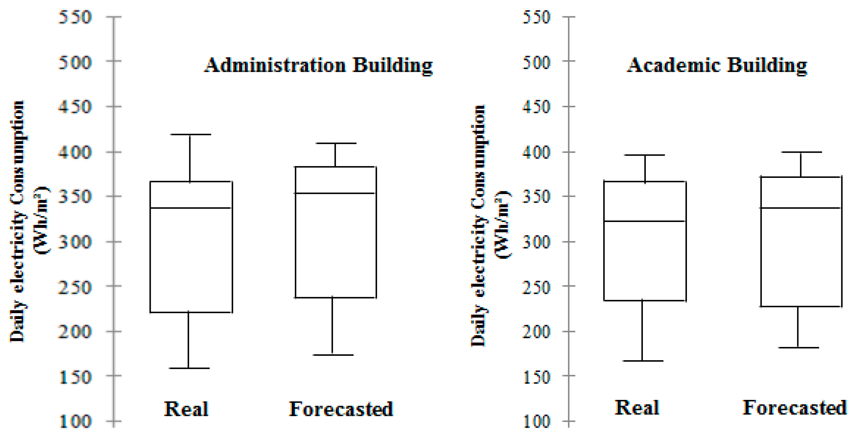
Table 7 demonstrates the comparison between real and forecasted daily electricity usage by using various statistical variables. It is clear from Table 7 that the difference between Max, Mean and Median values of real and predicted consumption for both the buildings is less than −5%. This authenticates the forecasting accuracy of the proposed model. Only in the case of ”minimum value”, the difference between real and forecasted values is somewhat considerable i.e., −12% and −10% for administrative and academic buildings respectively which shows that the base energy consumption values have dropped slightly. Overall, the difference between maximum, mean and median values of real and predicted electricity consumption for both buildings is negative which shows decrease in real energy consumption and demonstrates the improvement in energy ratings of both buildings.
Figure 9 presents a comparison between the real and predicted daily electricity usage (Wh/m2) in the form of box plots. This figure endorses the earlier results that the predicted energy consumption values are slightly higher than the real values.
4.1. Error Analysis of the Proposed MR Model
The proposed MR model has been assessed on the basis of the following two errors:
(i) NRMSE
The RMSE is a measure of the difference between values predicted/modelled and real values of the dependent variable. It is given by:
RMSE is further normalized by dividing with the range of observed data as shown in Equation (6):
(ii) Mean Absolute Percentage Error (MAPE)
This error is given by Equation (7):
where Yobs,i is the real value of daily electricity usage and Ypredicted,i is its forecasted value. Index “n” represents total number of observations.
Table 8 shows the error values and error % for both buildings. It is apparent that the model demonstrates promising results with a NRMSE of 12% and 13% for the administrative and academic building respectively. Similarly, the model offers a MAPE of 8.58% and 9.76% for administrative and academic buildings respectively. In both error analyses, the model performs slightly better for the administrative building compared to the academic building, however, the difference of error for predicting electricity consumption for two building types is minimal, i.e., 1%.
4.2. Limitations of the Proposed MR Model
The followings are the major limitations of this study:
- (i)
- In order for the model to behave correctly in future, the weights may need to be calculated again with new data. Since the MR method is fairly simple and quick, the weights may be calculated even every day (by adding yesterday’s data to previous data) and the model with new weights can be used to forecast energy consumptions of the following days.
- (ii)
- No real data was available for buildings occupancy and therefore, a proxy variable, i.e., weekday index has been used in order to compensate the effect of occupancy. Additional enhancement may be made in this model as long as occupancy data is on hands.
- (iii)
- Due to unavailability of data for similar types of buildings, this model has not been used to forecast daily electricity usage of any other similar buildings in the UK. Testing this model for similar buildings may open a window for further improvement.
- (iv)
- The model will work well provided the operating conditions remain same in the future. Any future change in building fabric, its operating schedule, equipment efficiency will require the revision of this model under new conditions.
5. Conclusions
In this study, we have developed a simple and reliable mathematical model for daily electricity usage forecasting for two major types of HE sector buildings. MR technique has been employed for the first time for development of a single electricity consumption forecasting model of two different types of buildings. Historical data of daily electricity usage of two buildings of London South Bank University have been regressed over normalized data of six variables, i.e., surrounding temperature, global irradiance, humidity, wind velocity, building type and, a proxy variable for building’s occupancy i.e., weekday index. The results of preliminary regression analysis have showed that except wind velocity which was dropped all other variables were found to be significant. It was also found that global irradiance and humidity have high co-linearity with surrounding temperature, therefore, these two variables were eliminated.
The model has been tested against real daily electricity consumption data of the same two subject buildings for year 2011 and it was found that the difference between real and predicted statistical values (max, mean, and median) was less than 8% which demonstrates the effectiveness of the proposed model. Moreover, NRMSE are observed to be low for the two buildings (i.e., 12% for administrative building and 13% for academic building) which further strengthens the effectiveness of the proposed model.
Acknowledgments
Authors would like to offer special gratitude to the Energy Manager, Anuj Saush at LSBU for providing information and electricity data.
Author Contributions
Khuram Pervez Amber and Muhammad Waqar Aslam conceived the idea and performed the experiments. Anzar Mahmood and Anila Kousar contributed in the write up of the manuscript and also gave useful insights during experimental analysis. Muhammad Yamin Younis and Bilal Akbar prepared the relevant graphics and tables after the experiments and contributed in the writing of description of these graphics and tables. Ghulam Qadar Chaudhary and Syed Kashif Hussain contributed during experimental analysis and gave useful comments for the improvement of the paper.
Conflicts of Interest
The authors declare no conflict of interest.
Acronyms
| AHU | Air Handling Unit |
| ANN | Artificial Neural Network |
| BMS | Building Management System |
| CHP | Combined Heat and Power |
| CRC | Carbon Reduction Commitment |
| CVRMSE | Coefficient of Variation of the Root-Mean-Square Error |
| DEC | Display Energy Certificate |
| GA | Genetic Algorithm |
| GIA | Gross Internal Area |
| HE | Higher Education |
| HEFCE | Higher Education Funding Council for England |
| HESA | Higher Education Statistics Agency |
| ISO | International Organization for Standardization |
| kWh | Kilo Watt Hour |
| LSBU | London South Bank University |
| MAPE | Mean Absolute Percentage Error |
| MR | Multiple Regression |
| NMBE | Normalized Mean Biased Error |
| NRMSE | Normalized Root Mean Square Error |
| NWD | Non-Working Day |
| RMSE | Root Mean Square Error |
| WD | Working Day |
References
- Hawkins, D.; Hong, S.M.; Raslan, R.; Mumovic, D.; Hanna, S. Determinants of energy use in UK higher education buildings using statistical and artificial neural network methods. Int. J. Sustain. Built Environ. 2012, 1, 50–63. [Google Scholar] [CrossRef]
- Higher Education Statistics Agency. Environmental Information, Estates Management Statistics Tables. Available online: https://www.hesa.ac.uk/index.php?option=com_heicontacts&Itemid=87 (accessed on 10 October 2016).
- Amber, K.P.; John, P. Barriers to the uptake of combined heat and power technology in the UK higher education sector. Int. J. Sustain. Environ. 2015, 34, 406–416. [Google Scholar] [CrossRef]
- Higher Education Statistics Agency. Environmental Information, Estates Management Statistics Tables. Available online: http://www.hesa.ac.uk/index.php?option=comdatatables&Itemid=121&task=showcategory&catdex=4 (accessed on 10 October 2016).
- Flams, J. English Universities Fall Further Behind Carbon Reduction Target, The World University Ranking. 2015. Available online: https://www.timeshighereducation.com/news/english-universities-fall-further-behind-carbon-reduction-target (accessed on 8 October 2016).
- Amber, K.P.; Aslam, M.W.; Hussain, S.K. Electricity consumption forecasting models for administration buildings of the UK higher education sector. Energy Build. 2015, 90, 127–136. [Google Scholar] [CrossRef]
- Chand, S. The Importance of Forecasting in the Operations of Modern Management. 2016. Available online: http://www.youtharticlelibrary.com/management/the-importance-of-forecasting-in-the-operations-of-modern-management/3504/ (accessed on 26 September 2016).
- Government Finance Administratives Association. Financial Forecasting in the Budget Preparation Process. 2014. Available online: http://www.gfoa.org/financial-forecasting-budget-preparation-process (accessed on 11 October 2016).
- Khan, A.R.; Mahmood, A.; Safdar, A.; Khan, Z.A.; Khan, N.A. Load forecasting, dynamic pricing and DSC in smart grid: A review. Renew. Sustain. Energy Rev. 2016, 54, 1311–1322. [Google Scholar] [CrossRef]
- Fumo, N.; Rafe, B.M.A. Regression analysis for prediction of residential energy consumption. Renew. Sustain. Energy Rev. 2015, 47, 332–343. [Google Scholar] [CrossRef]
- Braun, M.R.; Altan, H.; Beck, S.B.M. Using regressin analysis to predict the future energy consumption of a supermarket in the UK. Appl. Energy 2014, 130, 305–313. [Google Scholar] [CrossRef]
- Catalina, T.; Vlad, I.; Bogdan, C. Multiple regression model for fast prediction of the heating energy demand. Energy Build. 2013, 57, 302–312. [Google Scholar] [CrossRef]
- Amber, K.P. Development of a Combined Heat and Power Sizing Model for the Higher Education Sector of the United Kingdom. Ph.D Thesis, London South Bank University, London, UK, 2013. Available online: http://ethos.bl.uk/OrderDetails.do?uin=uk.bl.ethos.587546 (accessed on 11 October 2017).
- Kaza, N. Understanding the spectrum of residential energy consumption: A quantile regression approach. Energy Policy 2010, 38, 6574–6585. [Google Scholar] [CrossRef]
- Lomet, A.; Frederic, S.; David, C. Statistical modelling for real domestic hot water consumption forecasting. Energy Procedia 2015, 70, 379–387. [Google Scholar] [CrossRef]
- Alfonso, A. Multiple regression models to predict the annual energy consumption in the Spanish banking sector. Energy Build. 2012, 49, 380–387. [Google Scholar]
- Wang, H. Short-term prediction of power consumption for large-scale public buildings based on regression algorithm. Procedia Eng. 2015, 121, 1318–1325. [Google Scholar] [CrossRef]
- Sandels, C. Day-ahead predictions of electricity consumption in a Swedish administrative building from weather, occupancy, and temporal data. Energy Build. 2015, 108, 279–290. [Google Scholar] [CrossRef]
- Li, Q. Calibration of dynamic building energy models with multiple responses using Bayesian Inference and Linear Regression models. Energy Procedia 2015, 78, 979–984. [Google Scholar] [CrossRef]
- Fan, H.; MacGill, I.F.; Sproul, A.B. Statistical analysis of driving factors of residential energy demand in the preater Sydney region, Aurstralia. Energy Build. 2015, 105, 9–25. [Google Scholar] [CrossRef]
- Crompton, P.; Yanrui, W. Energy consumption in China: Past trends and future directions. Energy Econ. 2005, 27, 195–208. [Google Scholar] [CrossRef]
- Amiri, S.S.; Mottahedi, M.; Asadi, S. Using multiple regression analysis to develop energy consumption indicators for commercial buildings in the US. Energy Build. 2015, 109, 209–216. [Google Scholar] [CrossRef]
- Mastrucci, A.; Baume, O.; Stazi, F.; Leopold, U. Estimating energy savings for the residential building stock of an entire city: A GIS-based statistical downscaling approach applied to Rotterdam. Energy Build. 2014, 75, 358–367. [Google Scholar] [CrossRef]
- Saush, A.; (London South Bank University, London, UK). Personal communicaion, 2011.
- Capozzoli, A.; Daniele, G.; Francesco, C. Estimation models of heating energy consumption in schools for local authorities planning. Energy Build. 2015, 105, 302–313. [Google Scholar] [CrossRef] [Green Version]
- KCL London Air. Environmental Research Group. 2013. Available online: http://www.londonair.org.uk/ (accessed on 2 February 2013).
- Xiang, C.; Zhe, T. Impact of climate change on building heating energy consumption in Tianjin. Front. Energy 2013, 7, 518–524. [Google Scholar] [CrossRef]
- Liu, L.; Patrik, R.; Bahram, M. LCC assessments and environmental impacts on the energy renovation of a multi-family building from the 1980s. Energy Build. 2016, 133, 823–833. [Google Scholar] [CrossRef]
- Lu, S.; Zheng, S.; Kong, S. The performance analysis of administrative building energy consumption in the west of Inner Mongolia Autonomous Region, China. Energy Build. 2016, 127, 499–511. [Google Scholar] [CrossRef]
- Shibuya, T.; Croxford, B. The effect of climate change on administrative building energy consumption in Japan. Energy Build. 2016, 117, 149–159. [Google Scholar] [CrossRef]
- Liu, J.; Bing, L.; He, L.; Gao, Y. Investigation on the winter building energy consumption in rural areas in Jinan, China. In Proceedings of the 9th International Symposium on Heating, Ventilation and Air Conditioning (ISHVAC) Joint with Third international conference on Building Energy and Environment (COBEE), Tianjin, China, 12–15 July 2015. [Google Scholar]
- Pisello, A.L.; Castaldo, V.L.; Taylor, J.E.; Cotana, F. The impact of natural ventilation on building energy requirement at inter-building scale. Energy Build. 2016, 127, 870–883. [Google Scholar] [CrossRef]
- Amber, K.P.; Aslam, M.W. Energy-related environmental and economic performance analysis of two different types of electrically heated student residence halls. Int. J. Sustain. Energy 2016, 1–16. [Google Scholar] [CrossRef]
- Al-Garni, A.Z.; Syed, M.Z.; Javeed, S.N. A regression model for electric-energy-consumption forecasting in Eastern Saudi Arabia. Energy 1994, 19, 1043–1049. [Google Scholar] [CrossRef]
- Shen, P.; Malkawi, A.M. Impacts of climate change on US building energy use by using downscaled hourly future weather data. Energy Build. 2016, in press. [Google Scholar]
- Project Briatain Bank Holidays. 2012. Available online: http://projectbritain.com/bankholidays.html (accessed on 18 January 2013).
- Wang, L.; Mathew, P.; Pang, X. Uncertainties in energy consumption introduced by building operations and weather for a medium-size administrative building. Energy Build. 2012, 53, 152–158. [Google Scholar] [CrossRef]
- Sergios, T.; Konstantinos, K. Pattern Recognition; Elsevier Inc.: Orlando, FL, USA, 2009. [Google Scholar]
- Aslam, M.W. Pattern Recognition Using Genetic Programming for Classification of Diabetes and Modulation Data. Ph.D. Thesis, The University of Liverpool, Liverpool, UK, 2013. [Google Scholar]
Figure 1.
Variation of CO2 emissions of England’s HE sector [4].
Figure 1.
Variation of CO2 emissions of England’s HE sector [4].
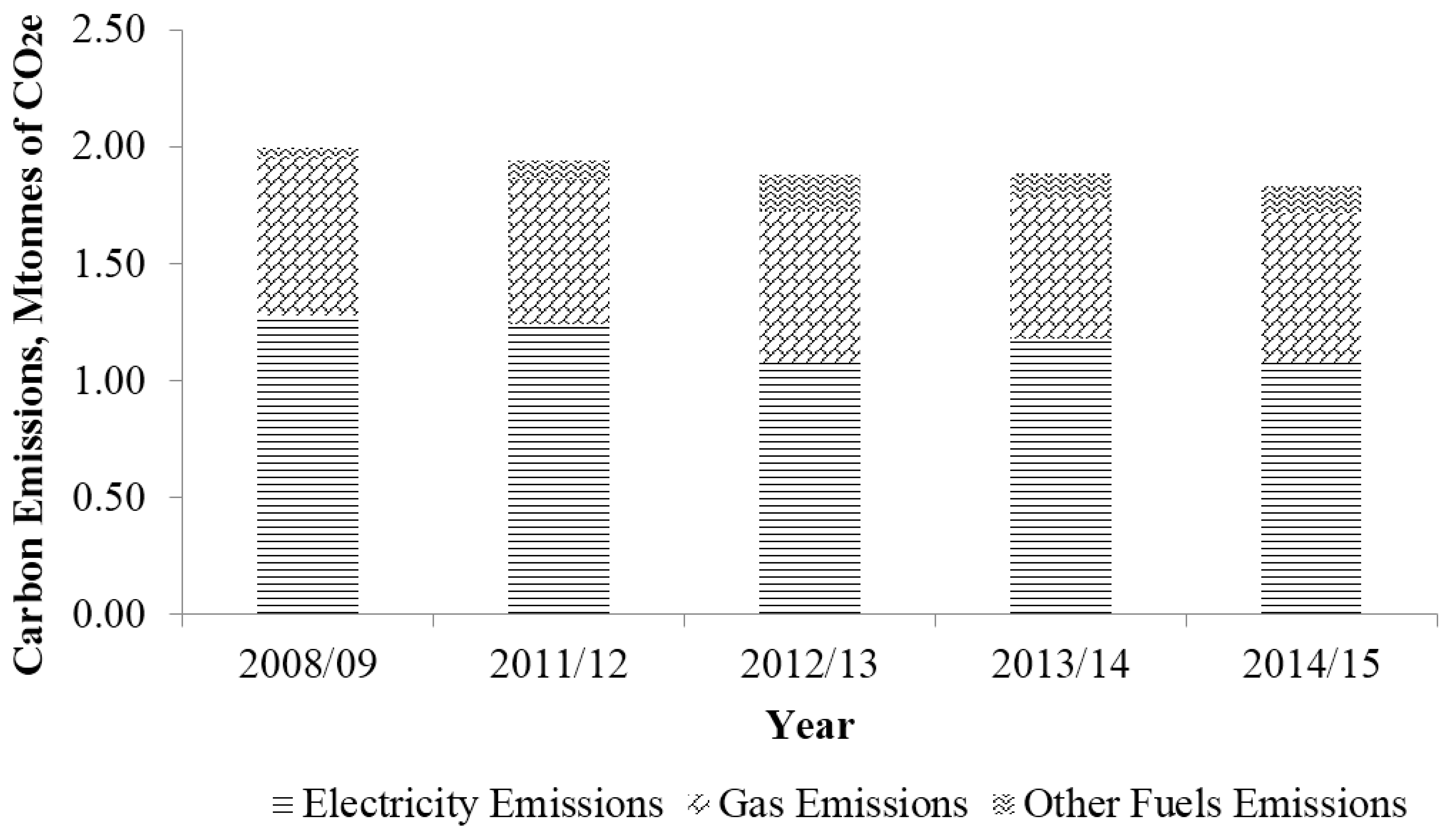
Figure 2.
Variation of annual electricity consumption of England’s HE sector [4].
Figure 2.
Variation of annual electricity consumption of England’s HE sector [4].
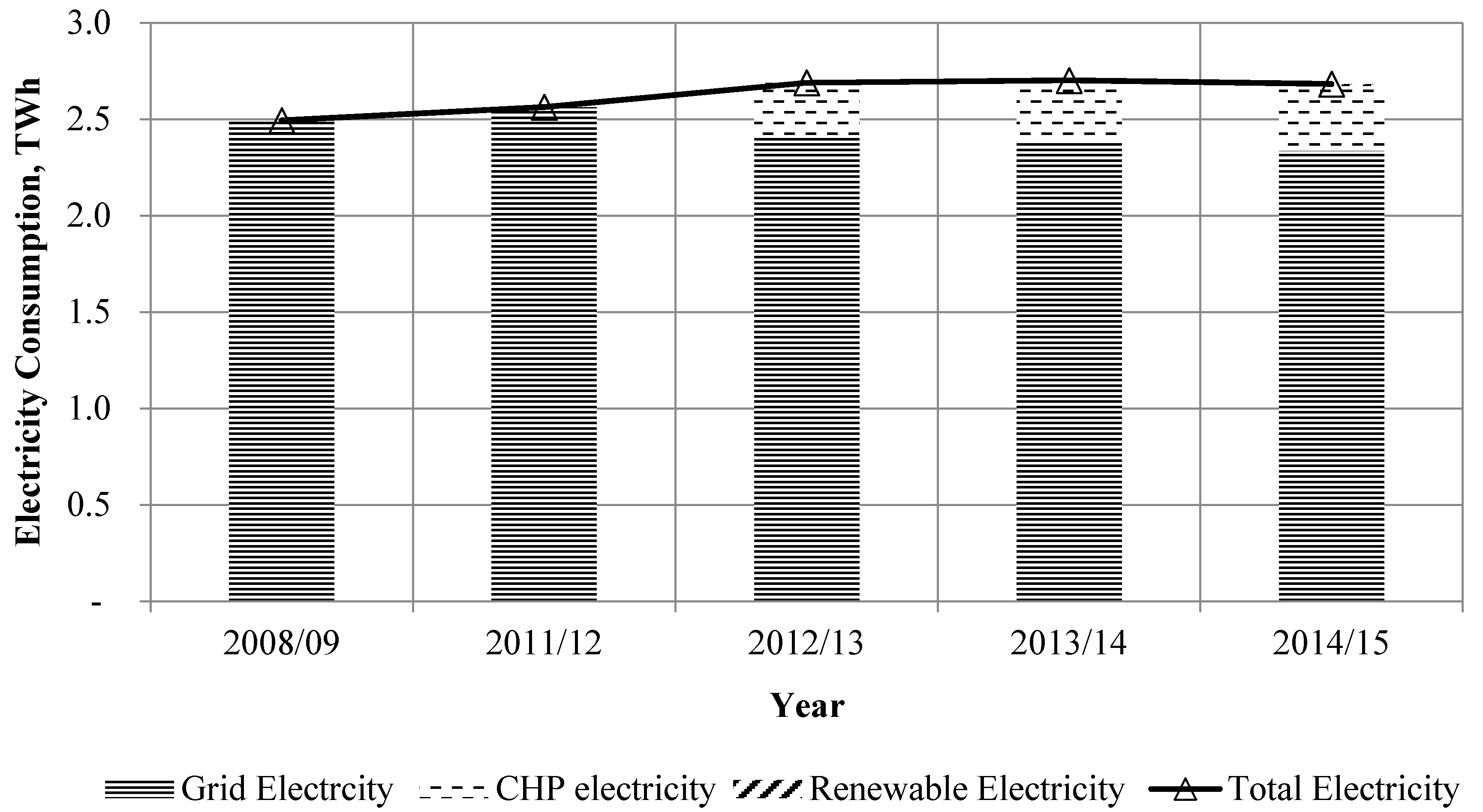
Figure 3.
Variation of annual gas consumption of England’s HE sector [4].
Figure 3.
Variation of annual gas consumption of England’s HE sector [4].

Figure 4.
Variation of annual CO2 Emissions of LSBU [4].
Figure 4.
Variation of annual CO2 Emissions of LSBU [4].
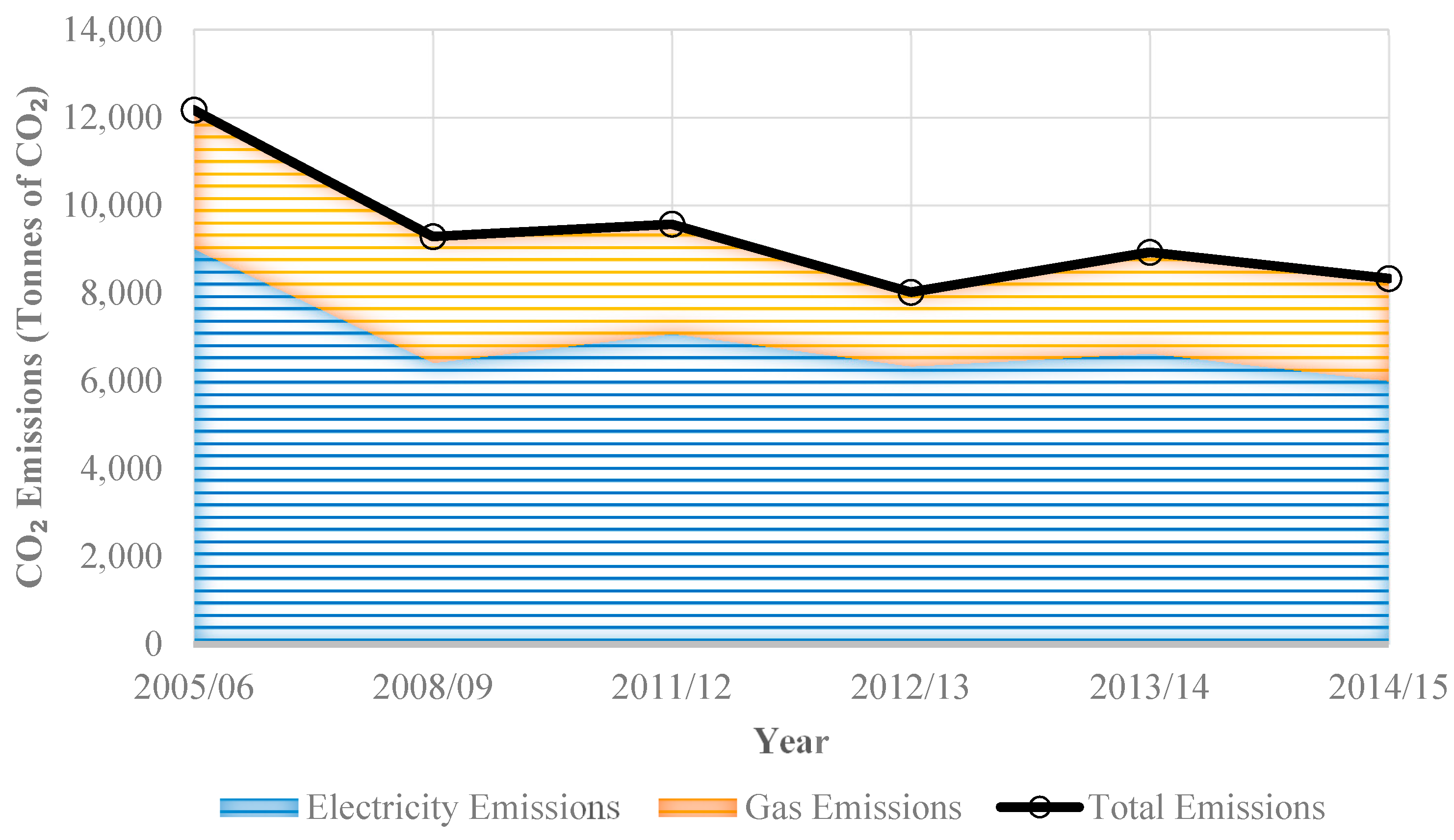
Figure 5.
Proposed methodology.

Figure 6.
Variation in daily electricity consumption of office and academic buildings [26].
Figure 6.
Variation in daily electricity consumption of office and academic buildings [26].

Figure 7.
Variation in daily mean values of weather parameters [26].
Figure 7.
Variation in daily mean values of weather parameters [26].
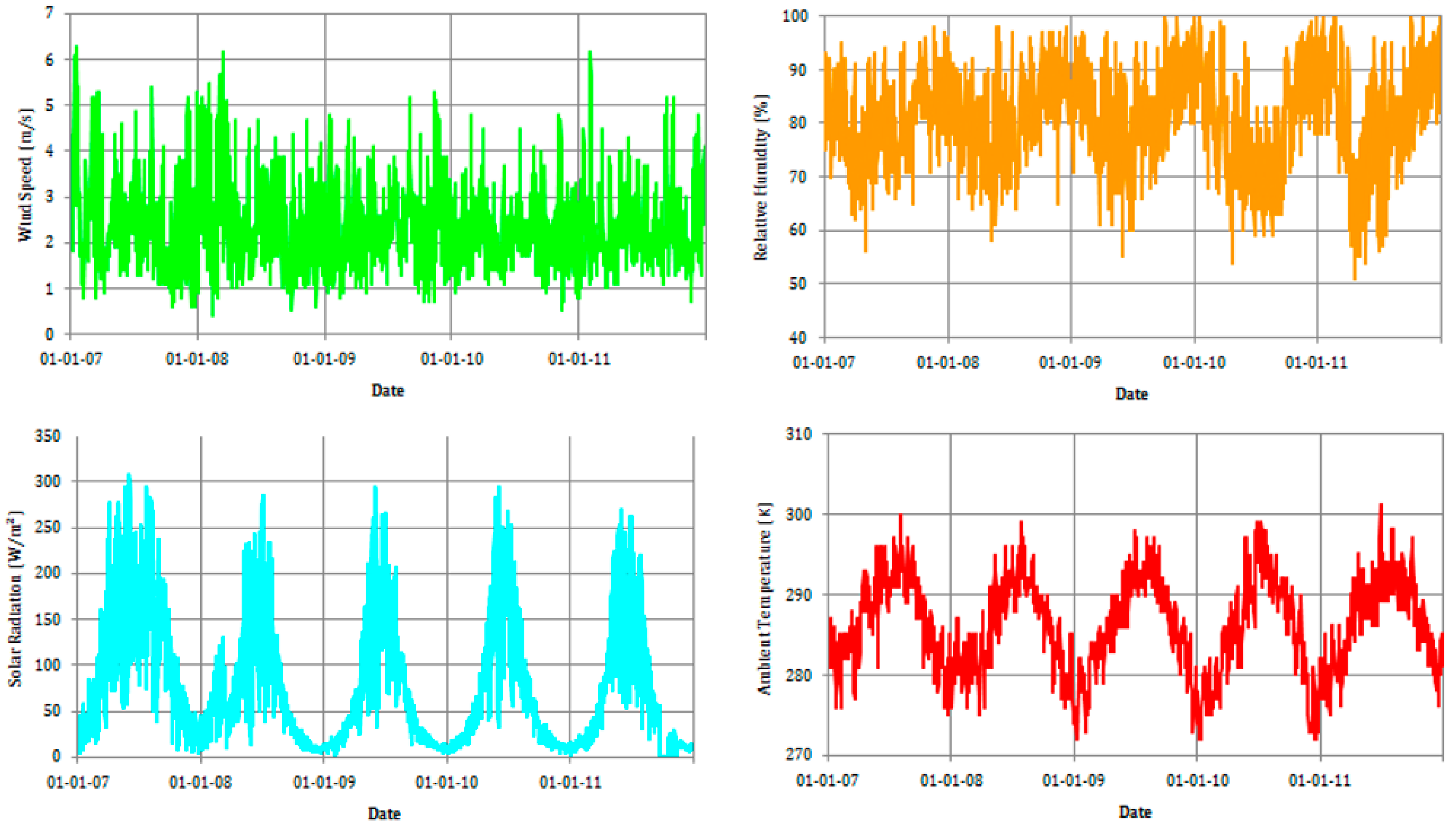
Figure 8.
Variation in annual working and non-working days [36].
Figure 8.
Variation in annual working and non-working days [36].

Figure 9.
Box plot comparison of real and predicted daily electricity consumption of two types of buildings.
Figure 9.
Box plot comparison of real and predicted daily electricity consumption of two types of buildings.

Table 1.
Five years statistics for England’s Higher Education Sector.
| 2008/09 | 2011/12 | 2012/13 | 2013/14 | 2014/15 | |
|---|---|---|---|---|---|
| Number of Students (Millions) | 1.55 | 1.68 | 1.57 | 1.55 | 1.55 |
| Grid Electricity Consumption, TWh | 2.49 | 2.56 | 2.41 | 2.39 | 2.34 |
| CHP Electricity Consumption, TWh | - | - | 0.27 | 0.30 | 0.34 |
| Renewable Electricity Consumption, TWh | - | - | 0.01 | 0.01 | 0.01 |
| Total Electricity Consumption, TWh | 2.49 | 2.56 | 2.69 | 2.70 | 2.68 |
| Gas Consumption, TWh | 2.99 | 2.78 | 2.60 | 2.27 | 2.41 |
| CHP Gas Consumption, TWh | - | - | 0.92 | 0.97 | 1.01 |
| Total Gas Consumption, TWh | 2.99 | 2.78 | 3.53 | 3.24 | 3.42 |
| Total Energy Consumption, TWh | 5.98 | 5.84 | 6.38 | 5.86 | 6.05 |
| Grid Electricity Emissions, Mtonnes of CO2 | 1.28 | 1.24 | 1.08 | 1.18 | 1.08 |
| Gas Emissions, Mtonnes of CO2 | 0.67 | 0.63 | 0.65 | 0.60 | 0.63 |
| Other fuels Emissions, Mtonnes of CO2 | 0.05 | 0.08 | 0.16 | 0.11 | 0.12 |
| Total Emissions, Mtonnes of CO2 | 2.00 | 1.95 | 1.88 | 1.89 | 1.83 |
| GIA, Million square metres, Mm2 | 20.37 | 21.25 | 21.35 | 21.63 | 22.16 |
| Total Number of Buildings | 12,826 | 12,577 | 12,628 | 12,683 | 12,754 |
Table 2.
Important information related to office and academic building.
| Description | Office Building | Academic Building |
|---|---|---|
| Building type | Offices | Lecture rooms, offices |
| GIA, m2 | 7811 | 8588 |
| Building year | N/A | 2003 |
| Building Orientation | South-West | South-West |
| Operating hours | 8 a.m. to 6 p.m. | 7.30 a.m. to 8.00 p.m. |
| Closing time | 10 p.m. | 10 p.m. |
| Cooling method | Naturally ventilated with few dedicated split AC units | Naturally ventilated |
| Heating Equipment | Two gas fired boilers | Six gas fired boilers |
| Lighting Type | CFL | CFL |
| No. of Lifts | 2 | 2 |
| No. of LV supplies | 2 | 1 |
| No. of floors | 3 | 6 |
Table 3.
Statistics of electricity consumption (Wh/m2) on working and non-working days.
| Non-Working Day | Working Day | |||
|---|---|---|---|---|
| Office | Academic | Office | Academic | |
| Min | 155 | 127 | 229 | 168 |
| Max | 311 | 404 | 479 | 550 |
| Mean | 222 | 220 | 374 | 357 |
| Median | 221 | 204 | 375 | 349 |
| N | 577 | 577 | 1249 | 1249 |
Table 4.
Statistics of weather parameters dataset.
| Ambient Temperature, (K) | Solar Radiation (W/m2) | Relative Humidity (%) | Wind Speed (m/s) | |
|---|---|---|---|---|
| Min | 272 | 0 | 51 | 0 |
| Max | 301 | 307 | 100 | 6 |
| Mean | 286 | 79 | 81 | 2 |
| Median | 286 | 52 | 81 | 2 |
| St. Dev. | 5.92 | 70.45 | 8.91 | 0.97 |
| N | 1826 | 1826 | 1826 | 1826 |
Table 5.
Preliminary MR Model and Collinearity Analysis.
| Multiple Regression Model | Coefficients | Standard Error | t-Stat | p-Value | |||
|---|---|---|---|---|---|---|---|
| Preliminary MR Model | Intercept | 323.62 | 0.80 | 404.58 | 323.62 | ||
| Surrounding Temperature, x1 | −15.29 | 1.10 | −13.80 | <0.05 | |||
| Global Irradiance, x2 | −10.90 | 1.27 | −8.58 | <0.05 | |||
| Relative Humidity, x3 | −2.30 | 1.01 | −2.27 | <0.05 | |||
| Wind Velocity, x4 | −2.17 | 0.81 | −2.69 | >0.05 | |||
| Weekday Index 1, x5 | 67.47 | 0.81 | 84.31 | <0.05 | |||
| Building type 2, x6 | −6.37 | 0.80 | −7.96 | <0.05 | |||
| Regression Analysis | Multiple R: 0.85 | ||||||
| Adjusted R2: 0.73 | |||||||
| Standard Error: 43.24 | |||||||
| Collinearity Analysis | |||||||
| Y | x1 | x2 | x3 | x4 | x5 | x6 | |
| Y | 1.00 | −0.25 | −0.23 | 0.13 | −0.03 | 0.81 | −0.08 |
| x1 | −0.25 | 1.00 | 0.69 | −0.42 | −0.01 | 0.02 | 0.00 |
| x2 | 0.81 | 0.02 | 0.01 | 0.00 | −0.01 | 1.00 | 0.00 |
| x3 | −0.08 | 0.00 | 0.00 | 0.00 | 0.00 | 0.00 | 1.00 |
| x4 | −0.23 | 0.69 | 1.00 | −0.61 | −0.02 | 0.01 | 0.00 |
| x5 | 0.13 | −0.42 | −0.61 | 1.00 | −0.09 | 0.00 | 0.00 |
| x6 | −0.03 | −0.01 | −0.02 | −0.09 | 1.00 | −0.01 | 0.00 |
1 Weekday Index has a value of “1” for a working day and “0” for a non-working day; 2 Building type has a value of “1” for office building and a value of “2” for academic building.
Table 6.
Proposed MR Model for Administration and Academic Buildings.
| Multiple Regression Model | Coefficients | Standard Error | t-Stat | p-Value | |
|---|---|---|---|---|---|
| Final Proposed MR Model | Intercept | 323.62 | 0.81 | 399.4 | <0.05 |
| Surrounding Temperature, x1 | −21.87 | 0.81 | −26.98 | <0.05 | |
| Weekday Index, x5 | 67.49 | 0.81 | 83.24 | <0.05 | |
| Building type, x6 | −6.37 | 0.81 | −7.86 | <0.05 | |
| Regression Analysis | Multiple R: 0.85 | ||||
| R2: 0.72 | |||||
| Adjusted R2: 0.72 | |||||
| Standard Error: 43.84 | |||||
Table 7.
Statistics of real and forecasted electricity consumption (Wh/m2) for year 2011.
| Office Building | Academic Building | |||||
|---|---|---|---|---|---|---|
| Real | Forecast | Difference | Real | Forecast | Difference | |
| Min | 155 | 181 | −17% | 158 | 168 | −6% |
| Max | 426 | 423 | 1% | 390 | 410 | −5% |
| Mean | 311 | 330 | −6% | 299 | 317 | −6% |
| Median | 347 | 359 | −3% | 321 | 346 | −8% |
| N | 365 | 365 | 365 | 365 | ||
Table 8.
Error comparison of MR model.
| Error Type | Office Building | Academic Building |
|---|---|---|
| RMSE | 31 Wh/m2 | 33.5 Wh/m2 |
| NRMSE | 12.3% | 13% |
| MAPE | 8.58% | 9.76% |
© 2017 by the authors. Licensee MDPI, Basel, Switzerland. This article is an open access article distributed under the terms and conditions of the Creative Commons Attribution (CC BY) license (http://creativecommons.org/licenses/by/4.0/).
Share and Cite
MDPI and ACS Style
Amber, K.P.; Aslam, M.W.; Mahmood, A.; Kousar, A.; Younis, M.Y.; Akbar, B.; Chaudhary, G.Q.; Hussain, S.K. Energy Consumption Forecasting for University Sector Buildings. Energies 2017, 10, 1579. https://doi.org/10.3390/en10101579
AMA Style
Amber KP, Aslam MW, Mahmood A, Kousar A, Younis MY, Akbar B, Chaudhary GQ, Hussain SK. Energy Consumption Forecasting for University Sector Buildings. Energies. 2017; 10(10):1579. https://doi.org/10.3390/en10101579
Chicago/Turabian StyleAmber, Khuram Pervez, Muhammad Waqar Aslam, Anzar Mahmood, Anila Kousar, Muhammad Yamin Younis, Bilal Akbar, Ghulam Qadar Chaudhary, and Syed Kashif Hussain. 2017. "Energy Consumption Forecasting for University Sector Buildings" Energies 10, no. 10: 1579. https://doi.org/10.3390/en10101579
Note that from the first issue of 2016, this journal uses article numbers instead of page numbers. See further details here.