Sensitivity Analysis to Control the Far-Wake Unsteadiness Behind Turbines


1
ETSIAE (School of Aeronautics)—Universidad Politécnica de Madrid, Pza Cardenal Cisneros 3, E-28040 Madrid, Spain
2
Center for Computational Simulation—Universidad Politécnica de Madrid, Boadilla del Monte, E-28660 Madrid, Spain
3
Department of Aerospace and Mechanical Engineering, University of Arizona, Tucson, AZ 85721, USA
*
Author to whom correspondence should be addressed.
Energies 2017, 10(10), 1599; https://doi.org/10.3390/en10101599
Submission received: 19 August 2017
/
Revised: 9 October 2017
/
Accepted: 10 October 2017
/
Published: 13 October 2017
(This article belongs to the Collection Wind Turbines)
Abstract
:We explore the stability of wakes arising from 2D flow actuators based on linear momentum actuator disc theory. We use stability and sensitivity analysis (using adjoints) to show that the wake stability is controlled by the Reynolds number and the thrust force (or flow resistance) applied through the turbine. First, we report that decreasing the thrust force has a comparable stabilising effect to a decrease in Reynolds numbers (based on the turbine diameter). Second, a discrete sensitivity analysis identifies two regions for suitable placement of flow control forcing, one close to the turbines and one far downstream. Third, we show that adding a localised control force, in the regions identified by the sensitivity analysis, stabilises the wake. Particularly, locating the control forcing close to the turbines results in an enhanced stabilisation such that the wake remains steady for significantly higher Reynolds numbers or turbine thrusts. The analysis of the controlled flow fields confirms that modifying the velocity gradient close to the turbine is more efficient to stabilise the wake than controlling the wake far downstream. The analysis is performed for the first flow bifurcation (at low Reynolds numbers) which serves as a foundation of the stabilization technique but the control strategy is tested at higher Reynolds numbers in the final section of the paper, showing enhanced stability for a turbulent flow case.
1. Introduction
The prediction and control of unsteady wakes is of capital importance in engineering applications since unsteady wakes and associated fluctuating forces are often correlated to undesired phenomena, such as unpredictable unsteady forces (e.g., dynamic stall), reduced fatigue life or noise generation. Some of these effects can undermine the structural integrity and reduce the operating life of the device and hence its prediction and control is paramount. An example is wind and tidal turbines for energy generation which are typically distributed in clusters or farms [1]. Ideally, the spacing between arrays of devices should be small to allocate a maximum number of turbines in a minimum space, which should maximise energy extraction. However, locating devices close to each other may not only limit the energy extracted by shadowing effects, but can also lead to problems of wakes interacting with neighbouring devices [1,2]. Therefore, the control of the wake unsteadiness may enhance energy production, alleviate structural damage and extend the turbine life.
The study of the onset of unsteady flow features can be performed using linear instability analysis [3]. Over the last decades, flow instability analysis has become a powerful tool to understand the onset of flow bifurcations leading to unstable (e.g., unsteady, periodic or chaotic) flow regimes. Flow instability techniques predict how small flow perturbations grow or decay with respect to an equilibrium flow solution (the base flow), providing information about the onset of unsteadiness, the physical instability mechanism and the means by which to control it. The control of unsteady features utilises sensitivity analysis [4,5] and identifies the regions of the flow that, if modified, lead to the greatest damping (or amplification) of unsteady features. The numerical study of flow sensitivity relies on the use of adjoint solutions [6]. The importance of adjoints and sensitivity maps, together with the mathematical machinery required for the study of the sensitive flow regions to different parameters, has been studied by various groups including the authors [7,8,9,10]. Having determined the most sensitive flow regions, it becomes easy to apply a flow control technique. Passive control introduces inactive objects (e.g., a small cylinder), which modify the flow to stabilise (or if needed destabilise) particular flow features [5,11]. Active control requires some source of external energy to modify the flow (e.g., blowing or suction) and can also be studied using linear instability [12]. Note that nonlinear control has been proposed [13] but is not considered here.
In this work, we model turbines using a localised flow resistance and passive flow control to enhance the stability of the wake arising from the turbines and based on linear momentum actuator disc theory (LMADT) by Rankine [14] and Froude [15] (see additional details in the Methodology Section). LMADT provides a model to simulate rotors that provide thrust (e.g., propellers or helicopters) or that extract energy from the flow stream (e.g., wind or tidal turbines). These models for simplified rotors provide an useful framework for the analysis of wake stability with a lower computational cost compared to simulating rotating blades. Indeed, the actuator disc can be used to estimate the aerodynamic forcing exerted by the turbine on the flow, whilst the far field is computed using a Navier–Stokes solver [16,17,18]. With this configuration, the wake resulting from modelled turbines can evolve freely and its stability analysed.
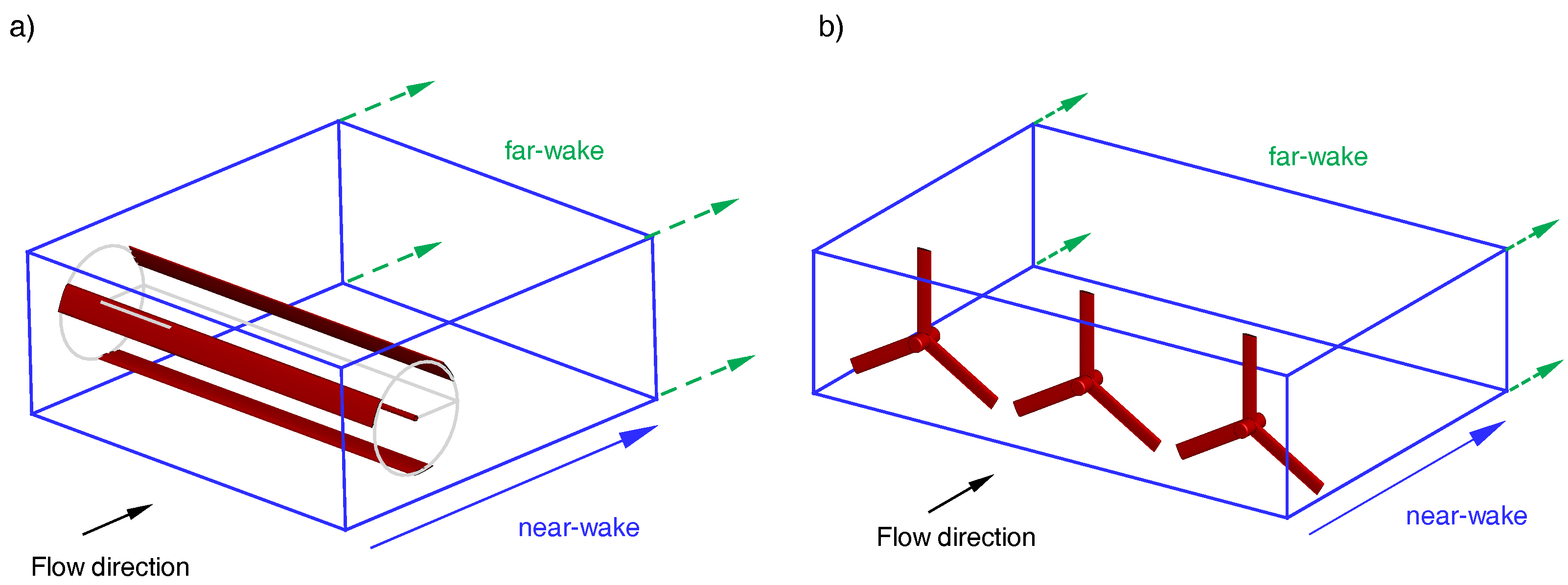
Turbine wakes show typically two distinct regions, a near and a far wake [2]. The near wake is highly influenced by the turbine geometry and is characterised by complex interactions between tip and hub vortices [19,20,21]. The far wake (starting 2 to 4 diameters downstream) shows more homogeneous averaged flow fields with Gaussian shapes and a centreline deficit that decays monotonically. This region is only weakly dependent on the turbine geometry [2] and hub vortex [20,21,22]. One of the advantages of the LMADT approach is that the complexity of the near-wake is hidden in the model, enabling the analysis of simplified far-wakes, e.g., neglecting tip/hub vortices and complex 3 dimensional effects. Bearing these simplifications in mind, turbines can be modelled using an LMADT actuator [17,18]. Two configurations, where the LMADT model may be used to model far-wakes are sketched in Figure 1. Figure 1a shows a three bladed cross-flow turbine and has been proposed for tidal farms in shallow water environments [23], whilst Figure 1b represents densely packed wind turbines, as discussed in [24,25]. Experimental investigations using porous discs [26] support the latter approximation since for discs in close proximity (∼0.5 diameters), it was shown that the individual near-wakes merged leading to a singular far-wake with a Gaussian lateral profile that persisted far downstream (>4 diameters downstream). Other studies, e.g., [27,28], have also suggested that simplified models may provide a fair approximation to the wake arising in realistic turbines. Therefore, the actuator disc approach remains a fundamental tool for the development of simplified models for wind energy harvesting. For example, simple modelling of wind farms often use actuator discs without rotational effects or swirl to predict power extraction [1,2]. Hence, the study of the stability of the actuator wake may be seen of engineering interest. Previous work [29,30] have used actuator discs, as simplified models, to study low-frequency far-wake phenomena such as wake meandering.
Wake meandering has been defined as low frequency oscillations in the far-wake. Medici & Alfredsson [31] reported rhythmic meandering oscillations and linked this phenomenon to the classic instabilities of bluff body vortex shedding. Latter, Larsen et al. [32] attributed the previous oscillations to large turbine loadings and associated meandering to turbulent ambient flow conditions. España et al. [30] redefined meandering as random oscillations (not periodic) of the wind turbine wake and showed that this phenomenon may be generated when the turbulence length scales are larger than the wake width. Let us note that the two definitions, time periodic or random oscillation, are not exclusive but complementary and may obey at the selection of parameters that control the system (e.g., turbulence flow conditions).
In this work, we retain the original definition by Medici & Alfredsson [31] to show that the far-wake may undergo time periodic oscillations and explore its control. We restrict the analysis to 2D wakes (or homogeneous in the out of plane direction). This simplification enables a deeper analysis of the two selected parameters to study the wake stability: the Reynolds number and the turbine thrust (or actuator forcing).
We show that an increase in the thrust provides a comparable effect to an increase in Reynolds, such that one may act on the rotor forcing to control the wake unsteadiness. In addition, using sensitivity analysis, we determine the flow regions that, when altered, provide stabilisation. Using localised control, we find configurations with enhanced stability. This work is novel and provides means to stabilise the wake arising from turbines. The study detailed here provides guidelines to defer the onset of wake unsteadiness (using passive control) such that the wake remains steady for significantly higher Reynolds numbers or turbine thrust. The study is carried out at low Reynolds numbers and for the first flow bifurcation. However, in the final section of the paper, we apply the control strategy to higher Reynolds numbers and also observe a stabilising effect of the wake.
The paper is organised as follows. First, we briefly describe the turbine model. Second, we introduce the mathematical machinery for instability, adjoints and sensitivity analysis. Third, we show the results obtained for a range of flow conditions and detail the procedure utilised to stabilise the wake. Fourth, the control strategy is applied to higher Reynolds numbers to show the effectiveness in more realistic flow conditions.
2. Methodology
2.1. Turbine Modelling
The linear momentum actuator disc theory often referred to as momentum theory or actuator disc theory was first introduced by Rankine [14] and Froude [15] to model ship propellers and subsequently extended by Lanchester [33] and Betz [34], who derived limits on the efficiency for this model. More recently, the theory has been particularised to model helicopter rotors [35], centrifugal pumps, turbochargers and wind turbines [36]. Over the last decade, the rise of new engineering devices for energy extraction, such as tidal turbines, have required the modification of classic theories to accommodate for blockage effects due to flow confinement (between sea surface and the ground) [37,38]. More sophisticated rotor models exist, e.g., [36,39], but we select LMADT since it provides the essential requirement to develop wake control strategies.
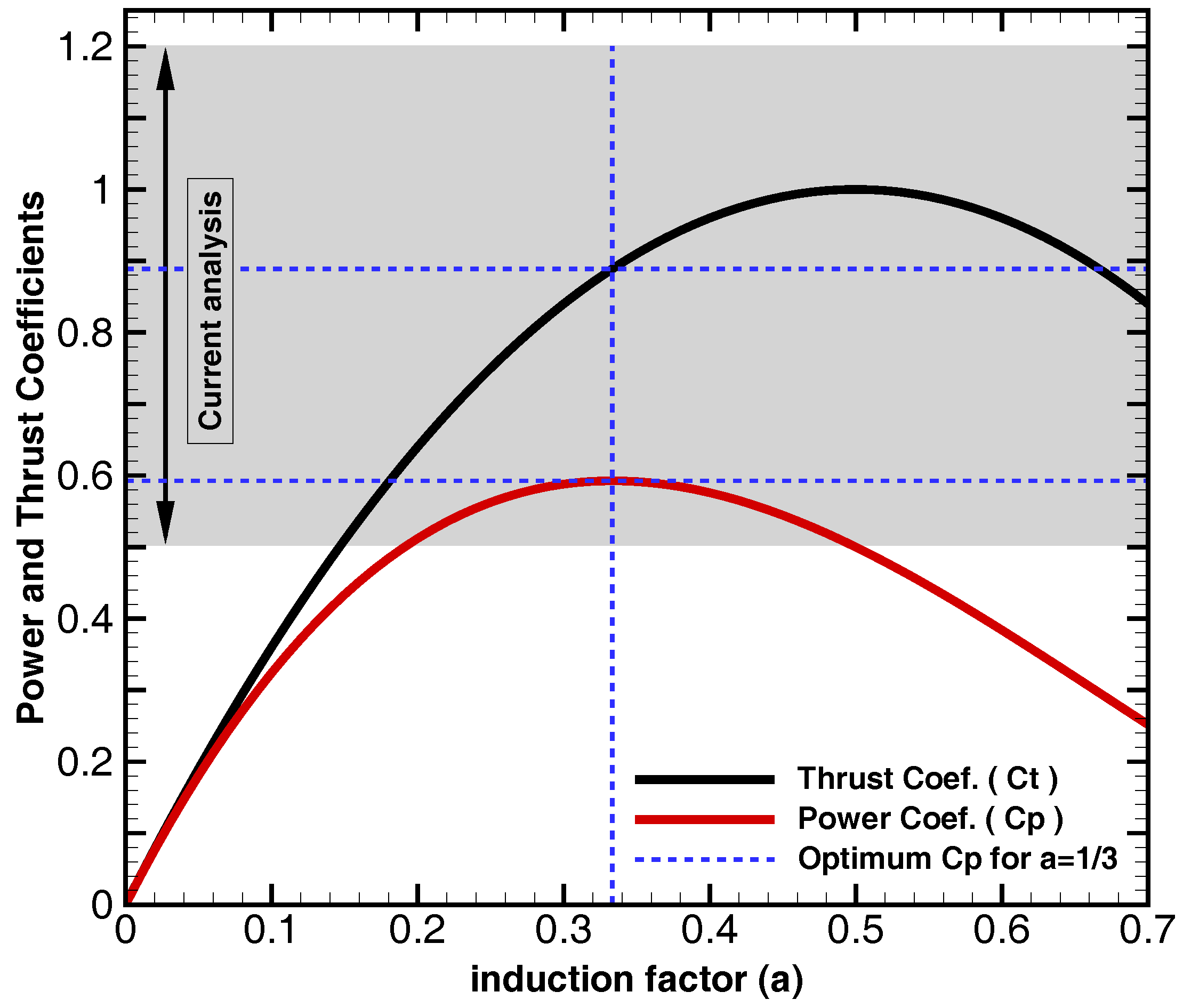
Let us briefly summarise the linear momentum actuator disc theory to provide context to our study. The theory [36] includes the derivation of the coefficients of power () and thrust () for an actuator disc. In the idealised inviscid and steady case, these are functions of the axial induction factor a, that relates to the deceleration of the flow through the disc, such that , where is the velocity of the flow aft the disc and is the velocity in the unperturbed upstream far field. Using mass, momentum-force conservation and Bernoulli’s principle, one can derive the following expressions for the power and thrust coefficients. These functions are depicted in Figure 2. Using LMADT, Betz [34] derived the maximum power that can be extracted from the flow. To do so, it suffices to differentiate and equate to zero the above mentioned expression for the power coefficient to obtain the optimal induction and corresponding maximum power coefficient with associated thrust coefficient . In addition, the theory bounds the thrust coefficient for idealised flows.
Our numerical study comprises cases for encompassing the thrust optimum (). Slightly larger thrust coefficients are considered to account for non-ideal flows that include viscous losses, see Section 3.6 in [36] or [40]. The range considered for this study is depicted in Figure 2. Using the LMADT expressions, we can relate the thrust values to induction factors of and power coefficients of . For larger values (), it is not possible to approximate the induction factor and power using the above LMADT identities. However, experiments and enhanced simulations (including viscosity) have show n that values above the limit are common; examples can be found in [36].
Without loss of generality, we only consider cases where the force applied by the turbine is uniform and constant (i.e., LMADT) but note that other theories that account for radial variations though the rotor may be used (e.g., Glauert rotor [36,41]). Indeed, the methodology conforms to an arbitrary shaped turbine forcing.
In the LMADT model, the thrust and the incoming velocity are constant. Even when considering these parameter as constants, we observe unsteady wakes for certain combinations of flow parameters and provide control of these flows. These unsteady wakes arise from the wake instability and not from a time varying thrust or incoming velocity.
2.2. Discrete Linear Instability Analysis
We consider a fully discrete approach to derive sensitivity fields [7,42]. The discrete method starts by discretising the governing equations to subsequently derive the linearised system; as opposed to first linearising to then discretise (i.e., continuous approach). An advantage of the discrete version is that, being purely algebraic, it does not require the derivation of adjoint equations or adjoint boundary conditions since these are automatically included in the matrix system. However, we note that both continuous and discrete formulations should provide analogous results. Comparisons between discrete and continuous approaches may be found elsewhere [6,43]. In addition, we note that the stability analysis presented here does not assume any parallel or weakly parallel flow assumption as it is of global type.
The methodology may be implemented in compressible or incompressible flow solvers. Here, we select, without loss of generality, a compressible version of the Navier–Stokes equations, where conservative variables are utilised: , where denotes the density, u and v are the velocity components in 2D and e denotes energy (see further details in Section 2.5). We start by considering a spatially discretised time varying and non-dimensional system
where is a discrete non-linear operator, is the mass matrix resulting from the spatial discretisation and denotes an turbine or actuator disc force. We have considered that the turbine thrust (or actuator forcing) depends on the flow field and will derive a suitable formulation for such cases. However, in the examples we will only consider constant forcing as defined in the LMADT approach such that if the streamwise momentum equation is modified in a 2D compressible solver. In the compressible Navier–Stokes equations, denotes the divergence of the viscous and convective fluxes. It is convenient to proceed by redefining
To perform linear instability analysis, the state variable is decomposed into its steady state contribution, , and a small unsteady perturbation, such that . We proceed by inserting this decomposition into Equation (2) and linearise the non-linear discrete system using Taylor series (around ). Subtracting the base flow equation and neglecting second order terms (), we obtain a linearised and time varying system for the perturbation field
with denoting the Jacobian matrix. We include a detailed derivation in an Appendix A of this text. Note that for a constant turbine thrust (independent of ), the Jacobian simplifies to . Equation (3) may be advanced in time to simulate the growth or decay of perturbation upon [8,44].Alternatively, it is possible to solve the above perturbation equation in the frequency domain by introducing the ansatz, , which leads to an eigenvalue problem
The eigenvector is the direct mode associated to the complex eigenvalue, , whose real and imaginary components represent the perturbation growth rate and angular frequency. The Jacobian matrix can be computed numerically using for example a complex step approximation [45] and first used for stability analysis by the authors [7]. In this approach, a complex Taylor expansion (with imaginary increment) is considered to derive an approximation for the matrix derivatives (e.g., ). The complex method has favourable properties in that the relative error decays with second order (requiring only one function evaluation) and that it eliminates subtractive errors often seen in second order approximations.To extract the eigenvalues and eigenvectors from a shift and invert Arnoldi algorithm is employed.
To provide a sense of the spectrum of eigenvalues, we provide an example in Figure 3, for the uncontrolled actuator at with , see details in Section 3. From the cloud of eigenvalues, which are all stable in this case (since they all have negative growth ), we will select the least stable (see Figure 3b) and closest to zero-growth (horizontal red dashed line) to control unsteady flow features. It will be latter seen that this mode governs the wake stability. Note that the horizontal coordinate provides the angular frequency () associated to the each modal flow structure. The aim of this work is to control or decrease the growth rate associated to the unstable eigenvalue, which is equivalent to stabilising the flow.
An estimate for the smallest flow feature that can be resolved by the numerical method is provided but the highest imaginary part of the eigenspectra (highest frequency), which in our case is 30 Hz (not shown in Figure 3). Note that the figures, included in this work, depict the angular frequency and need to be divided by to obtain the previous value. Assuming a unitary phase velocity, the minimum resolvable wavelength is 0.03 m. The most critical eigenvalues studied using our solver and meshes have a frequency of 0.47 Hz and associated wavelengths (assuming unitary phase velocity) of 2 m, which can be accurately resolved since our precision is 0.03 m.
2.3. Discrete Adjoints
We define a discrete adjoint eigenvalue problem by selecting the inner product in the computational domain , such that , for and continuous vectors associated to their discrete versions and , where is again the mass matrix (as in Equation (2)) and () denotes the Hermitian transpose. Then, the discrete adjoint Jacobian matrix follows . Expanding this expression and using the definition for the discrete inner product, it is easy to see that the discrete adjoint Jacobian matrix is . In our case, the Jacobian is real and . In summary, the adjoint modes can be obtained by solving , with .
2.4. Discrete Sensitivities
Sensitivity analysis can be used to locate the flow regions that are more sensitive to flow modifications. The most sensitive regions define the “sweet spots” for the location of a passive control mechanism. In this work, we consider the sensitivity of the eigenvalue subject to a modification of the base flow, , or steady forcing, . These were first derived for the continuous approach [5] and recently extended to the discrete approach [7,42].The resulting sensitivity fields , , can be obtained following the method of Lagrangian multipliers, which aim at maximising the change in the eigenvalue growth rate, , subject to perturbations and base flow constraints. The mathematical derivation can be found in [7,42] and only the final expressions for the sensitivities to base flow and external localised forcing are provided:
Here, is the adjoint of the base flow and is the discrete adjoint of the sensitivity matrix , which is obtained when differentiating the Jacobian multiplied by the direct mode corresponding to the least stable (or closest to the unstable region) eigenvalue with respect to the base flow: . The computation of the sensitivity matrix, , is again performed using a complex step approximation [7].
2.5. Numerical Flow Solutions Using a High Order Method
To simulate the turbine wakes, we use a nodal variant of a high order discontinuous Galerkin (DG) technique that can be modified to accommodate for the body force that models the turbine. High order methods (order ≥ 3) are characterised by low numerical errors (i.e., dispersion and diffusion) and their ability to use mesh refinement (increased number of mesh nodes or h-refinement) and/or polynomial enrichment (p-refinement) to achieve more accurate solutions [46,47]. The latter p-refinement method provides an exponential decay of the numerical error rather than the typical algebraic decay yielded by h-refinement solvers.
The compressible Navier–Stokes equations can be discretised using the DG approach, on a quad mesh (h-mesh) using polynomial spaces (p-mesh) of arbitrary order within each computational element. The temporal terms are discretised using a third order Runge-Kutta method and are converged until steady state, which is reached once the infinite norm of the conservation law residual (for all flow equations) falls below a tolerance not larger than . The Mach number is selected low, M = 0.2, such that compressibility effects are negligible. Details of the numerical solver may be found in [46,47,48].
2.6. Summary of the Methodology for Stability and Sensitivity Analysis
The methodology to perform stability and sensitivity analysis can be summarised in the following 4 steps:
- Compute a steady base flow using a numerical solver. High order h/p methods are preferred to obtain find solutions with low numerical errors. We time march the compressible Navier–Stokes Equations (1), until the residual falls below . If we do not obtain convergence, the case is considered unstable and we do not perform the stability analysis.
- Having computed all direct eigenvalues/eigenvectors, we select the least stable and compute its adjoint, see Section 2.3.
- With the direct and adjoint modes, it is possible to compute the Hessian matrix associated to the sensitivities detailed in Section 2.4. Subsequently, the sensitivities to base flow modifications and to localised forcing can be calculated using Equations (5).
The resulting sensitivities guide the design of passive control to stabilise the turbine wake.
3. Results
3.1. Preliminaries
The analysis is performed for the first flow bifurcation (at low Reynolds numbers) which serves as a foundation of the stabilization technique but the control strategy is tested at higher Reynolds numbers in the final section of the paper, showing enhanced stability for a turbulent flow case.
The left domain boundary is of Dirichlet type with uniform inflow for the streamwise velocity whilst the upper, right and lower boundaries are treated with a Neumann outflow boundaries to minimise blockage effects. The zoomed region, in Figure 4, details the location where the forcing term is applied (in red) and shows the effective degrees of freedoms for the high order technique.
We illustrate the destabilising effect of increasing the Reynolds number (based on the turbine diameter and free stream velocity) in Figure 4. Figure 4a,c depicts the streamwise velocity field and the vorticity magnitude for a stable case at Re and , whilst Figure 4b,d shows an unsteady wake for Re = 3500 and .
For the steady case, we plot, in Figure 5, the pressure and streamwise velocity distribution along the mid-plane and passing through the turbine issued from the DG solver. It can be seen that the pressure jump is localised within the turbine region whilst the effect on the streamwise velocity spreads upstream and downstream of the turbine. Note that these simulated results are similar to the propositions of the actuator disc theory [35,36]. In addition, it is possible to check that the body force () relates to a pressure drop such that , where is the pressure jump, denotes the fluid density and the free stream velocity. The latter expression is a strict equality only when considering inviscid flows and becomes an approximation for viscous solutions.
Additionally, and to provide a wider context to this study, we include results for pressure and velocity computed using the commercial solver Ansys-Fluent-16.2 [49], in Figure 5. This solver is selected to simulate inviscid, time averaged flows without turbulence models (“no-model” or laminar mode) and simulations using the k-epsilon model at various Reynolds numbers. We compare these results to our high order DG results at Re = 3000. We observe that our DG results agree very well with the inviscid case and laminar simulations (without turbulence model) at both studied Reynolds numbers (Re = 3000 and Re ), in terms of wake recovery. Wake mixing is enhanced when using turbulence models that account for ambient turbulence. Wake recovery is highly influenced by the turbulence parameters but reaches the inviscid or no-model case for low ambient turbulence (e.g., turbulence intensity of 0.1%). These comparisons suggest that our DG laminar cases that consider the first bifurcation at low Reynolds numbers may cover a wider spectra of cases, and that the results here reported may be extrapolated to inviscid and turbulent regimes with low ambient turbulence levels. In what follows, we consider high order DG results for the analysis. However, in the last section of the paper, we will return to explore the stability of turbulent wakes.
3.2. Mesh Convergence
We perform a convergence study for the least stable eigenvalue rather than on the steady base flows because we find that small errors, that do not affect the base flow (which is converged when the residual is below for all polynomial orders), can result in noticeable discrepancies in the eigenvalues (i.e., perturbation growth and frequency). We select the computational domain depicted in Figure 4 and vary the polynomial order in each element (p-order) fixing the turbine thrust and the Reynolds number Re = 1000. The h-mesh has 742 quadrilateral elements with polynomial orders ranging from to 5. Table 1 shows the convergence for the growth rate () and the angular frequency () associated to the least stable eigenmode for each polynomial order.
It can be seen that for we obtain unchanged results when compared to ; i.e., with a relative error smaller than in the growth rate. All the results presented in what follows have been obtained using , which results in meshes with 18,550 degrees of freedom.
Regarding the domain size, Giannetti & Luchini [4] showed that the region resulting from the overlap of direct and adjoint modes, i.e., The structural sensitivity or “wavemaker” region, determines the minimal extent of the computational domain for the modes to remain unchanged. As it will be shown in Section 3.5.1, our boundary conditions do not intersect with the structural sensitivity region. Consequently, the least stable mode, its adjoint and the conclusions extracted regarding their stability and control should not vary significantly for larger domains.
3.3. The Onset of Wake Unsteadiness
We consider a range of Reynolds numbers (), based on the rotor diameter D and the free stream velocity, from to 3500 and turbine thrust () from to 1.2. The simulated cases together with their wake behaviour (i.e., steady or unsteady) are summarised in Table 2. Note that all simulations are time marched using our unsteady solver and only if the infinite norm of the Navier–Stokes residual falls below , the flow is considered stable and steady. When the flow does not converge to a steady state, it is considered unstable and unsteady.
The table reports that for a fixed forcing a steady (stable) wake becomes unsteady (unstable) if the Reynolds number is increased from to . Alternatively, the table shows that for a fixed Reynolds number , an increase in the turbine thrust from to destabilises the wake.
Figure 6a–c presents streamwise velocity in sections parallel to the actuator at various streamwise locations for a steady () and an unsteady () case. Figure 4 and Figure 6 suggest a co-flow wake type as reported by Tammisola et al. [50] and Tammisola [51], who studied the effect of the Reynolds number and co-flow shear ratio (describing the strength of shear between fluids at inlet) in the stability and sensitivity patterns for global modes in jets and wakes.
In our work, we study the effect of the Reynolds number and the turbine thrust, which may be approximated as the co-flow shear ratio.
Since viscosity smooths the steep velocity gradients and enhances the velocity recovery in the wake, lower Reynolds numbers provide more stable wakes, as previously reported [50]. Similarly, a reduced turbine thrust results in smoother velocity gradients leading to enhanced stability. Ashton et al. [22] studied hub vortex instabilities and concluded that lower thrust also tend to stabilise the wake. Figure 6a–c shows that the velocity fields present a step gradient near the edge of the turbine that becomes smoother for sections further downstream. These gradients are smoother for decreased Reynolds numbers, which suggests a stabilising effect of the viscosity. Figure 6d presents the evolution of the vorticity magnitude along the line , which lies at the edge of the turbine and in the streamwise direction along the high vorticity region depicted in Figure 4c,d. For both and , the vorticity decays downstream of the turbine whereas for (unsteady case) the vorticity strongly oscillates aft 10 diameters downstream of the turbine. This suggests that the spatial onset of the primary instability is not at the edge of the turbine but 10 to 15 diameters downstream, this behaviour will explained later using stability analysis. Finally, the spatial location for the instability onset moves upstream for higher Reynolds number or higher turbine thrust. The aim of this work is to defer the onset of wake unsteadiness such that the wake remains steady for significantly higher Reynolds numbers or turbine thrust.
3.4. Stability Analysis
The complex eigenvalues are obtained from the direct eigenvalue problem as detailed in previous sections. As mentioned, when the system is said to be linearly unstable in time (i.e., absolute temporal instability). The evolution of the least stable (or more unstable) eigenvalue is presented in Figure 7a–d, when varying the Reynolds number () and the turbine thrust (). These figures confirm and quantify the destabilising effect of increasing the Reynolds number or the turbine thrust.
It can be seen that increasing the turbine thrust (e.g., extracting more energy using a wind turbine) has a destabilising effect on the wake, which is comparable to the destabilising effect of an increase in the Reynolds number. Note that for wind/tidal turbines there is little or no control over the Reynolds number as this is dictated by the environment. However, the thrust (or resistance) of the turbine can be modified by adjusting the speed at which its blades rotate. In addition, small variations are observed in the frequencies (imaginary part of the eigenvalues) when varying the Reynolds number or the turbine thrust, Figure 7b,d.
Second order polynomials are used to model the evolution of . We find the polynomials corresponding to Figure 7a and Figure 7c
Computing the roots of the polynomial provides an approximation of the critical values for Reynolds numbers and thrust for which the system becomes unstable. We find and . These estimates are validated by brute force computations to find that the wake becomes unsteady in the range (for ) and for (for ). Furthermore, taking derivatives of the models, we can obtain the sensitivity of the growth rates with respect to the Reynolds numbers and turbine thrust
When considering the operating point (Re = 3000, ), these sensitivities quantify that a variation of the turbine thrust has an equivalent effect to a variation of Reynolds number .
Let us note that we have selected quadratic polynomials since we needed to fit data ranging from 3 to 5 points. This model is only used to extrapolate the data to higher Re and values and to obtain sensitivity information (derivatives) with respect to these parameter to enrich the discussion throughout the manuscript. However, other characteristics of the model such as its implicit minimum/maximum or the lower root are not of interest as they do not have a physical meaning.
For completeness, Figure 8a,b depict the direct and adjoint streamwise-momentum components (real part), respectively, corresponding to the least stable eigenvalue for and . The direct mode shows that the perturbations begins past the turbine and that its amplitude grows exponentially downstream. The shape of this mode suggests that the wake may be divided in two regions: a middle-distance-wake, and a very-far-wake , , as observed in the previous section: vorticity curves in Figure 6 and the shape of the direct mode in Figure 8a. A spatial stability analysis performed using spatial-DMD [8,52,53,54] reveals a spatial growth of 0.4 for the middle-distance-wake and of 0.9 for the very-far-wake showing that the convective instability of the wake is enhanced aft 10 turbine diameters. The two distinct wake regions will lead to varying sensitivities (see next section). The adjoint mode propagates upstream, which is explained by the upstreaming advective nature of the adjoint equations [6].
3.5. Wake Control Using Sensitivity Analysis
3.5.1. Sensitivity Analysis
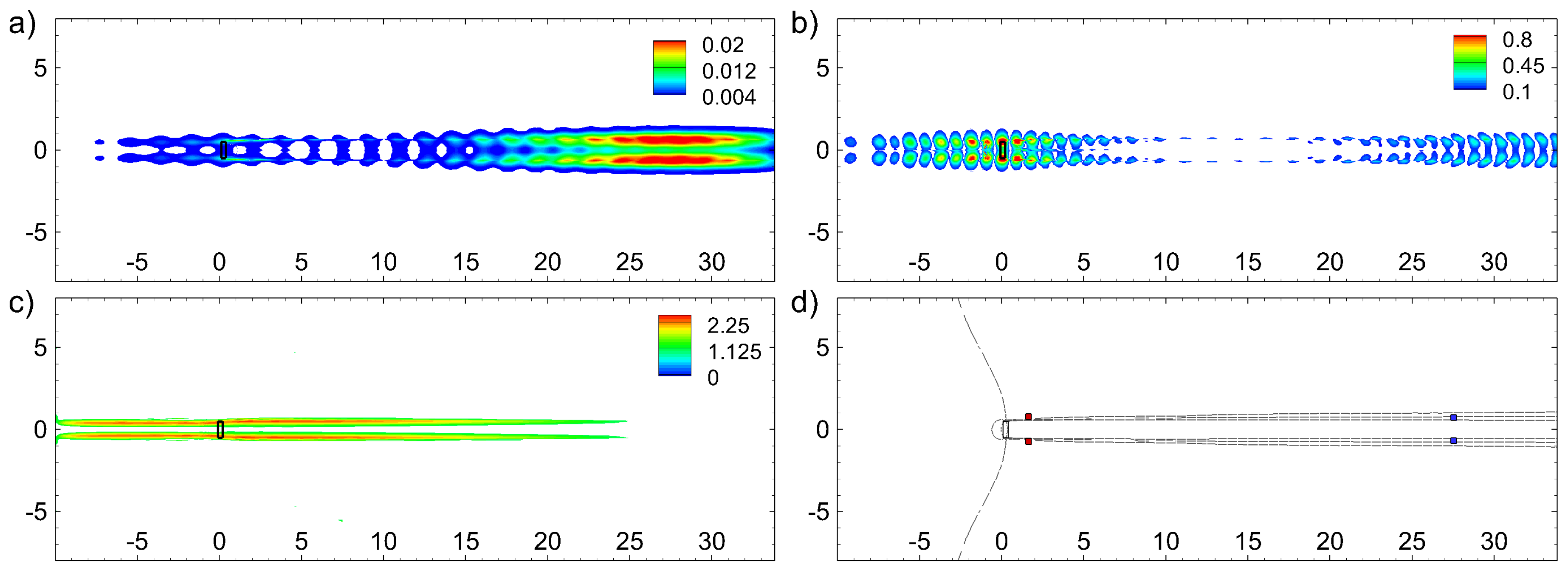
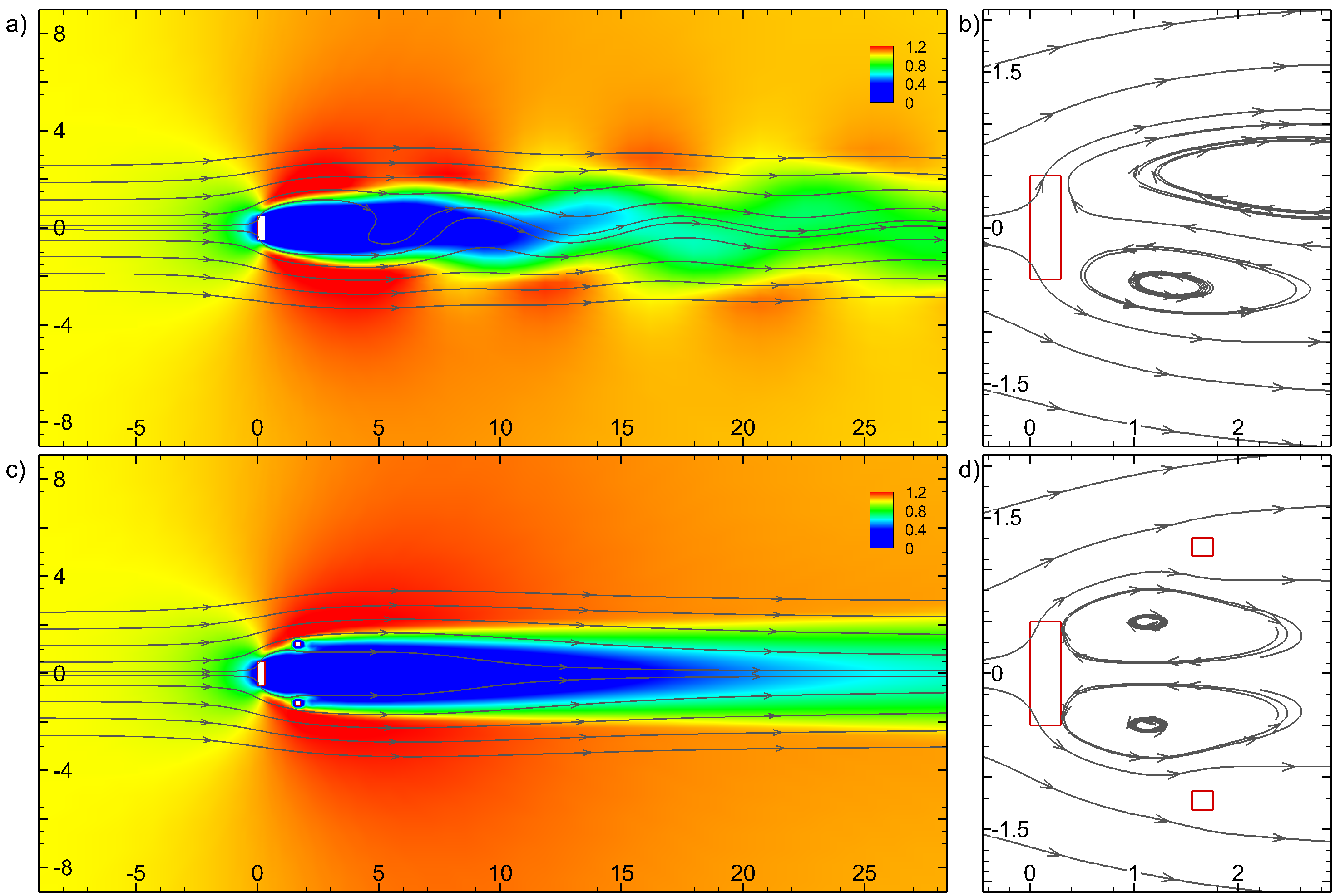
Our interest is in stabilising the least stable eigenvalue identified with linear instability analysis. In this section, we compare three sensitivities: the structural sensitivity, the sensitivities to base flow modifications and localised forcing. The structural sensitivity or “wavemaker” region [4] is shown in Figure 9a. This identifies the most sensitive regions to localized feedback and results from computing the scalar product of direct and adjoint modes.
Figure 9a shows that the wavemaker region becomes important in the region downstream of the turbine () and that a much smaller region appears near the edges of the turbine. These two distinct zones may be related to the near and far wake regions detected in the previous section.
Figure 9b reports the sensitivity to base flow modifications (real part of in Equation (5)) and confirms the two regions detected by the structural sensitivity. Before we present the sensitivity to a steady force, it is interesting to note the wavy shape of the two previous sensitivities. This oscillating behaviour has been reported before by Tammisola [51] and was attributed to an incompressible pressure feedback mechanism, where reflection of the mode can be in phase or out of phase leading to localised sensitivities. Additionally, it was argued that control mechanisms acting in these regions would not be robust.
In addition to the previous sensitivities, Figure 9c presents the sensitivity to a steady force (real part of in Equation (5)). The latter sensitivity detects a flow region closer to the turbine () and within the shear layer arising from the edges of the turbine.
In summary, two regions are determined by the sensitivity analysis. The first one is located far downstream of the turbine as indicated by the structural sensitivity and the sensitivity to base flow modifications. A second zone appears clearly when the sensitivity to a steady forcing is computed. Note that for engineering applications (e.g., wind turbines), having regions relatively close to the turbine is desirable as it eases the implementation of a passive control technique to stabilise the flow (e.g., control may be installed on the nacelle of the turbine).
3.5.2. Wake Stabilisation
To validate the methodology and provide guidelines for flow control of turbines, pointwise forces are placed in the regions identified by the various sensitivity contour maps. Two sets of forces (applied in the opposite direction to the freestream velocity) are incorporated: is located near the turbine at , whilst is situated far downstream , both within the shear layer region. The locations for and are shown in Figure 9d. The point forces have a non-dimensional magnitude of 1.0. Note that by considering only passive point forces, we can disregard the energy input into the system.
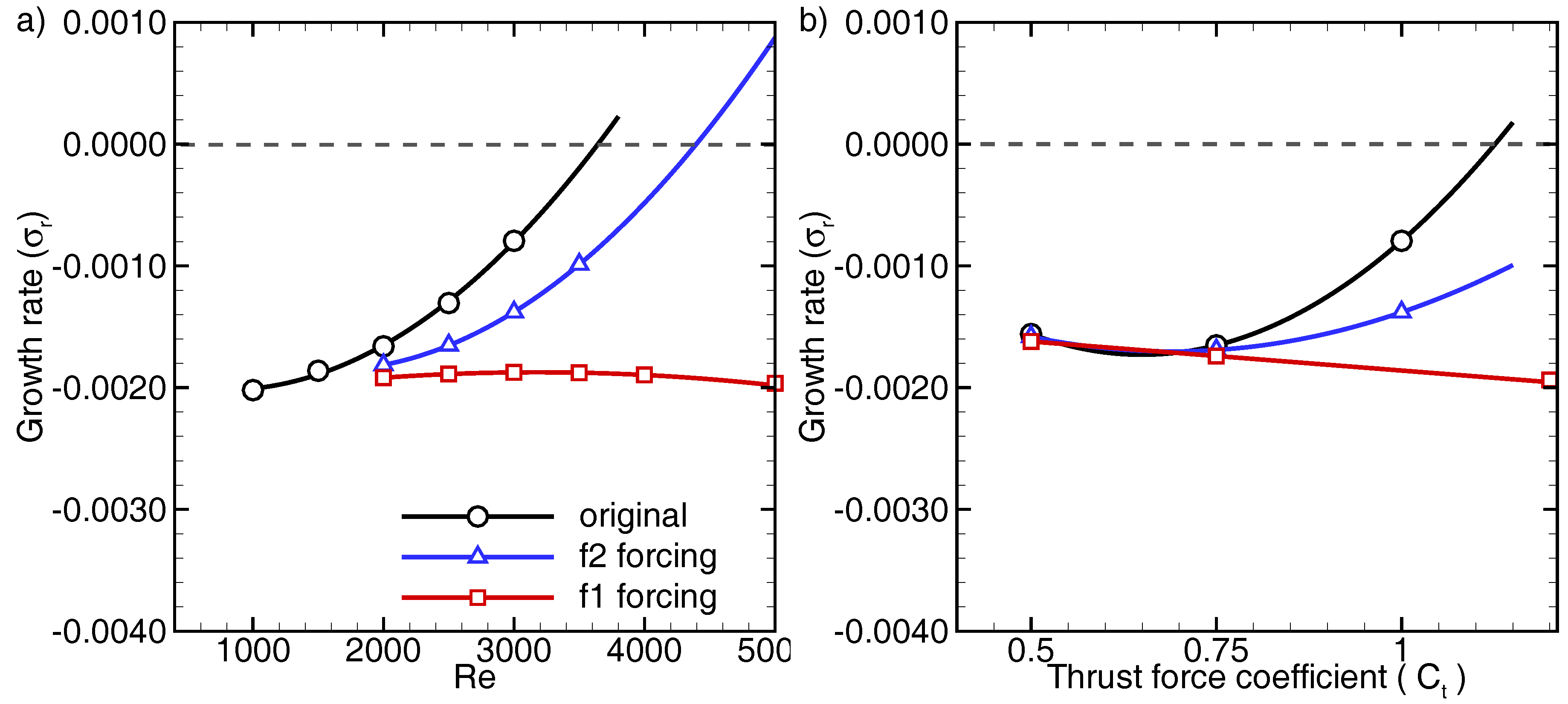
Growth rates for uncontrolled (original) and controlled cases and (applied separately) for a range of Reynolds numbers (with fixed turbine thrust ) are shown in Figure 10a, whilst growth rates for a variety of turbine thrust (at fixed ) are plotted in Figure 10b. The figures confirm that both controls and stabilise the wake considerably.
The effect of the near turbine control and the downstream control increases when increasing the Reynolds numbers or the turbine thrust, but shows a more effective stabilising effect for the range of Reynolds numbers and thrust considered. As for the uncontrolled case, we again fit second order polynomials to the data for the control
which predicts , quantifying the enhanced stabilisation by (the uncontrolled case showed ). For completeness, we compute the sensitivities of the growth rate () to a change in and turbine thrust () by taking derivatives of the models.
The percentage reduction in sensitivity to the Reynolds number is and to the turbine thrust , when compared to the uncontrolled cases (see Section 3.4). Again, we quantify these sensitivities by noting that a variation of the turbine thrust is now comparable to a variation of Reynolds number . In addition, let us note that the sensitivities for the control are close to zero, which follows from the curves being almost horizontal near and . For the control the wake becomes unsteady at and a different eigenmode is responsible of the instability.
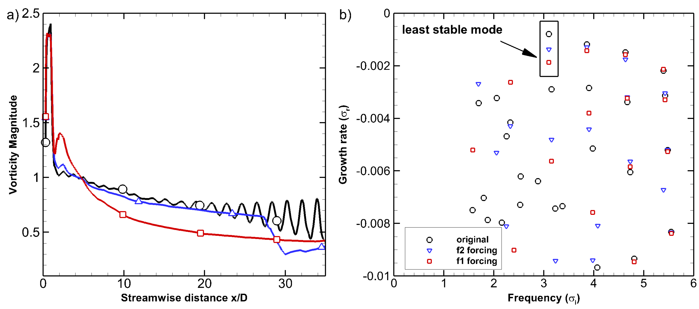
The mode shapes have been modified by the action of the control as illustrated in Figure 11, where we show the direct mode (real part streamwise momentum) for and for: uncontrolled (original), and cases. For the forcing, Figure 11b, it can be seen that the spatial growth of the least stable mode is reduced far downstream of the turbine when compared to the original uncontrolled mode Figure 11a. Particularly, the very-far-wake region () shows a decreased spatial growth with respect to the uncontrolled case. Indeed, the spatial-DMD provides, for the control, a convectively stable wake with a spatial growth of .
In addition, Figure 12b shows the complete eigenspectra (growth and frequency) for the uncontrolled and the controlled cases at Re = 3000 and . It can be seen that the control applied to stabilise the least stable mode may modify the stability of other modes (other frequencies) but that all remain in the stable region. Consequently, the stabilisation of the least stable mode results in an enhanced stability overall.
For completeness, we explore the changes in the vorticity and velocity distributions in the wake. Figure 12a reports the vorticity evolution for the modified turbine with the control forcing and to confirm the stabilising effect at the shear layer.
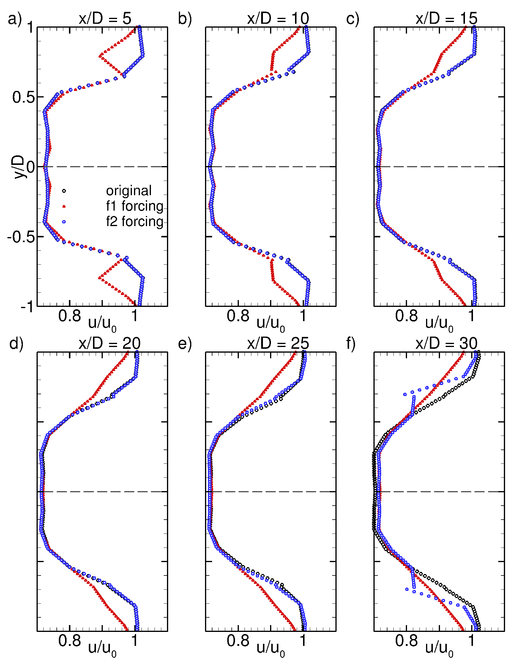
Finally, we report the streamwise velocity at downstream sections parallel to the turbine in Figure 13d for the original unsteady wake, and the controlled and at and . The case shows that the forcing initialises a smoother velocity gradient which has a stabilising effect on the wake, Figure 13a. A similar effect is seen for , Figure 13f, but the latter, which acts further downstream, results in a less efficient stabilisation mechanism. We conclude that the control located close to the turbine is best suited to enhance the stability of wakes arising from turbines.
4. Wake Control at Higher Reynolds Numbers
In this last section, we simulate an unsteady turbulent wake and show that the information extracted in previous sections can be used to design a passive control. We use the turbulent k-epsilon model of Ansys-Fluent. The Reynolds number is increased to Re (e.g., representing a wind turbine of diameter 2 m subject to a free stream velocity m/s) and the forcing to to enhance instabilities and associated wake unsteadiness. We select low turbulence levels (e.g., turbulence intensity ) since we observe that, for low turbulence levels, the wake has an increased tendency to unsteadiness.
Figure 14 shows the results of the unsteady wake (Figure 14a,b. When including a passive control similar to the previous (located near the turbine), the wake becomes steady, as shown in Figure 14c,d. In this turbulent conditions, the passive control is centered at , same downstream distance as the control (in the laminar case), but different location. We have moved the control away from the turbine to avoid the interaction with the shear layer, which is thicker in this turbulent case. Additionally, in this case, and to simplify the implementation, the controls are solid bodies and not pointwise forces. These solid bodies need to be small to avoid additional non-linearities (e.g., shedding from the controls) but their shape is not critical. The main objective of these devices is to deflect the outer shear layer of the wake, which results in an enhanced stability and a steady wake. We observe that the control (located near the turbine) modified for turbulent flows enhances the stability of the wake, showing that the analysis, formally derived for laminar flow, provides valuable information for Reynolds number of engineering interest. The resemblance of the wake profiles for varying Reynolds numbers when using LMADT (see Section 3.1 and Figure 5) is probably the reason as to why the control technique is useful at different flow regimes.
5. Conclusions
This work shows how to stabilise the wake arising from a 2D actuator that models wind/tidal turbines. The type of rhythmic oscillations, observed in this study, have been previously associated to the meandering phenomenon [31]. The stabilisation of unsteady wakes (and associated fluctuating forces) can alleviate damaging effects such as increased loads or noise generation. These effects can undermine the structural integrity and reduce the operating life of the turbines and hence its prediction and control is of great interest.
Using linear stability and sensitivity analysis based on adjoints, we find the regions of the flow that, when modified, provide a more stable wake. We test this procedure for a range of Reynolds numbers and turbine forcing (thrust) to show its usability at stabilising or delaying unsteadiness in the wake. It is shown that locating point forces close behind the disc modifies the shear layer profile stabilising the wake. This mechanism is more efficient that stabilising the wake far downstream. This result is interesting since locating passive control mechanisms close to the turbine is desirable as it eases its implementation and maintenance; for example, control may be installed on the nacelle of the turbine.
The analysis is performed for the first flow bifurcation at low Reynolds numbers but the control strategy is tested at higher Reynolds numbers and shows promise in enhancing the stability of the far wake for flows of engineering interest.
The current work has considered only 2D wakes and neglected 3D effects that may arise from circular rotors. Further work is necessary to assess the control of 3D wakes that include azimuthal instabilities or near-wake effects.
It is expected that the presented results provide guidelines for a wide range of engineering devices, where the linear momentum actuator disc theory (LMADT) holds such as wind and tidal turbines but also propellers or helicopter rotors.
Acknowledgments
The authors thank the European Commission for the financial support received through the project SSEMID: Stability and Sensitivity Methods for Industrial Design, under grant contract PITN-GA-675008.
Author Contributions
Esteban Ferrer and Eusebio Valero conceived the methods; Esteban Ferrer and Oliver M. F. Browne implemented the methods, Esteban Ferrer and Oliver M. F. Browne ran the simulations; Esteban Ferrer, Oliver M. F. Browne and Eusebio Valero analyzed the results; Esteban Ferrer wrote the paper.
Conflicts of Interest
The authors declare no conflict of interest.
Appendix A
Starting with the system
we introduce the state variable decomposition , to obtain
To linearise the non-linear operator , we use Taylor series (around ):
Neglecting second order terms (), and replacing Equation (A3) into Equation (A2), we obtain a linearised version of Equation (A2).
Finally, we may subtract the base flow equation: , to arrive at the final expression for the time evolution of perturbations:
References
- Stevens, R.J.A.M.; Meneveau, C. Flow Structure and Turbulence in Wind Farms. Annu. Rev. Fluid Mech. 2017, 49, 311–339. [Google Scholar] [CrossRef]
- Vermeer, L.J.; Sorensen, J.N.; Crespo, A. Wind turbine wake aerodynamics. Prog. Aerosp. Sci. 2003, 39, 467–510. [Google Scholar] [CrossRef]
- Schmid, P.; Henningson, D. Stability and Transition in Shear Flows; Springer: New York, NY, USA, 2001. [Google Scholar]
- Giannetti, F.; Luchini, P. Structural sensitivity of the first instability of the cylinder wake. J. Fluid Mech. 2007, 581, 167–197. [Google Scholar] [CrossRef]
- Marquet, O.; Sipp, D.; Jacquin, L. Sensitivity analysis and passive control of cylinder flow. J. Fluid Mech. 2008, 615, 221–252. [Google Scholar] [CrossRef]
- Luchini, P.; Bottaro, A. Adjoint Equations in Stability Analysis. Annu. Rev. Fluid Mech. 2014, 46, 493–517. [Google Scholar] [CrossRef]
- Browne, O.; Rubio, G.; Ferrer, E.; Valero, E. Sensitivity analysis to unsteady perturbations of complex flows: A discrete approach. Int. J. Numer. Methods Fluids 2014, 76, 1088–1110. [Google Scholar] [CrossRef]
- Ferrer, E.; de Vicente, J.; Valero, E. Low cost 3D global instability analysis and flow sensitivity based on dynamic mode decomposition and high-order numerical tools. Int. J. Numer. Methods Fluids 2014, 76, 169–184. [Google Scholar] [CrossRef]
- Iorio, M.C.; Gonzalez, L.M.; Ferrer, E. Direct and adjoint global stability analysis of turbulent transonic flows over a NACA0012 profile. Int. J. Numer. Methods Fluids 2014, 76, 147–168. [Google Scholar] [CrossRef] [Green Version]
- Gonzalez, L.M.; Ferrer, E.; Diaz-Ojeda, H.R. Onset of three dimensional flow instabilities in lid-driven circular cavities. Phys. Fluids 2017, 29, 064102. [Google Scholar] [CrossRef]
- Strykowski, P.; Sreenivasan, K. On the formation and suppression of vortex at low Reynolds numbers. J. Fluid Mech. 1990, 218, 71–107. [Google Scholar] [CrossRef]
- Meliga, P.; Sipp, D.; Chomaz, M. Effect of compressibility on the global stability of axisymmetric wake flows. J. Fluids Mech. 2010, 660, 499–526. [Google Scholar] [CrossRef] [Green Version]
- Mao, X.; Blackburn, H.; Sherwin, S. Nonlinear optimal suppression of vortex shedding from a circular cylinder. J. Fluids Mech. 2015, 775, 241–265. [Google Scholar] [CrossRef] [Green Version]
- Rankine, W. On the mechnical principles of the action of propellers. Trans. Inst. Nav. Archit. 1865, 6, 13–39. [Google Scholar]
- Froude, R. On the part played in propulsion by differences of fluid pressure. Trans. Inst. Nav. Archit. 1889, 30, 390–423. [Google Scholar]
- Sorensen, J.; Shen, W. Numerical Modeling of Wind Turbine Wakes. ASME J. Fluids Eng. 2002, 124, 393–399. [Google Scholar] [CrossRef]
- Mikkelsen, R. Actuator Disc Methods Applied to Wind Turbines. Ph.D. Thesis, Technical University of Denmark, Lyngby, Denmark, 2003. [Google Scholar]
- Porte-Agel, F.; Wu, Y.T.; Lu, H.; Conzemius, R.J. Large-eddy simulation of atmospheric boundary layer flow through wind turbines and wind farms. J. Wind Eng. Ind. Aerodyn. 2011, 99, 154–168. [Google Scholar] [CrossRef]
- Ivanell, S.; Mikkelsen, R.; Sørensen, J.N.; Henningson, D. Stability analysis of the tip vortices of a wind turbine. Wind Energy 2010, 13, 705–715. [Google Scholar] [CrossRef]
- Iungo, G.V.; Viola, F.; Camarri, S.; Porté-Agel, F.; Gallaire, F. Linear stability analysis of wind turbine wakes performed on wind tunnel measurements. J. Fluids Mech. 2013, 737, 499–526. [Google Scholar] [CrossRef]
- Viola, F.; Iungo, G.; Camarri, S.; Porté-Agel, F.; Gallaire, F. Prediction of the hub vortex instability in a wind turbine wake: Stability analysis with eddy-viscosity models calibrated on wind tunnel data. J. Fluids Mech. 2014, 750. [Google Scholar] [CrossRef]
- Ashton, R.; Viola, F.; Camarri, S.; Gallaire, F.; Iungo, G.V. Hub vortex instability within wind turbine wakes: Effects of wind turbulence, loading conditions, and blade aerodynamics. Phys. Rev. Fluids 2016, 1, 073603. [Google Scholar] [CrossRef]
- McAdam, R.A.; Houlsby, G.T.; Oldfield, M.L.G. Experimental measurements of the hydrodynamic performance and structural loading of the Transverse Horizontal Axis Water Turbine: Part 1. Renew. Energy 2013, 59, 105–114. [Google Scholar] [CrossRef]
- Draper, S.; Houlsby, G.T.; Oldfield, M.L.G.; Borthwick, A.G.L. Modelling tidal energy extraction in a depth-averaged coastal domain. IET Renew. Power Gener. 2010, 4, 545–554. [Google Scholar] [CrossRef] [Green Version]
- Draper, S.; Nishino, T.; Adcock, T.; Taylor, P. Performance of an ideal turbine in an inviscid shear flow. J. Fluids Mech. 2012, 796, 86–112. [Google Scholar] [CrossRef] [Green Version]
- Myers, L.E.; Bahaj, A.S. An experimental investigation simulating flow effects in first generation marine current energy converter arrays. Renew. Energy 2012, 37, 28–36. [Google Scholar] [CrossRef]
- Wu, Y.T.; Porte-Agel, F. Large-eddy simulation of wind-turbine wakes: Evaluation of turbine parametrisations. Bound. Layer Meteorol. 2011, 138, 345–366. [Google Scholar] [CrossRef]
- Aubrun, S.; Espana, G.; Loyer, S.; Hayden, P.; Hancock, P. Is the actuator disc concept sufficient to model the far-wake of a wind turbine? In Progress in Turbulence and Wind Energy IV; Springer: Berlin, Germany, 2012; pp. 227–230. [Google Scholar]
- Kang, S.; Yang, X.; Sotiropoulos, F. On the onset of wake meandering for an axial flow turbine in a turbulent open channel flow. J. Fluids Mech. 2014, 744, 376–403. [Google Scholar] [CrossRef]
- Espana, G.; Aubrun, S.; Loyer, S.; Devinant, P. Spatial study of the wake meandering using modelled wind turbines in a wind tunnel. Wind Energy 2011, 14, 923–937. [Google Scholar] [CrossRef]
- Medici, D.; Alfredsson, P.H. Measurements behind model wind turbines: Further evidence of wake meandering. Wind Energy 2008, 11, 211–217. [Google Scholar] [CrossRef]
- Larsen, G.C.; Madsen, H.A.; Thomsen, K.; Larsen, T.J. Wake meandering: A pragmatic approach. Wind Energy 2008, 11, 377–395. [Google Scholar] [CrossRef]
- Lanchester, F. A contribution to the theory of propulsion and the screw propeller. J. Am. Soc. Nav. Eng. 1915, 27, 509–510. [Google Scholar] [CrossRef]
- Betz, A. Das Maximum der theoretisch möglichen Ausnutzung des Windes durch Windmotoren. Z. Gesamte Turbinenwes. 1920, 26, 307–309. [Google Scholar]
- Leishman, G. Principles of Helicopter Aerodynamics (Cambridge Aerospace Series), 2nd ed.; Cambridge University Press: Cambridge, UK, 2006. [Google Scholar]
- Burton, T.D.; Sharpe, N.J.; Bossanyi, E. Wind Energy Handbook; John Wiley & Sons Ltd.: West Sussex, UK, 2011. [Google Scholar]
- Whelan, J.; Graham, J.; Peiro, J. A free-surface and blockage correction for tidal turbines. J. Fluids Mech. 2009, 624, 281–291. [Google Scholar] [CrossRef]
- Nishino, T.; Willden, R. The efficiency of an array of tidal turbines partially blocking a wide channel. J. Fluids Mech. 2012, 708, 596–606. [Google Scholar] [CrossRef]
- Duong, M.Q.; Grimaccia, F.; Leva, S.; Mussetta, M.; Le, K.H. Improving Transient Stability in a Grid-Connected Squirrel-Cage Induction Generator Wind Turbine System Using a Fuzzy Logic Controller. Energies 2015, 8, 6328–6349. [Google Scholar] [CrossRef] [Green Version]
- Munters, W.; Meyers, J. An optimal control framework for dynamic induction control of wind farms and their interaction with the atmospheric boundary layer. Philos. Trans. R. Soc. A Math. Phys. Eng. Sci. 2017, 375. [Google Scholar] [CrossRef] [PubMed]
- Smith, D.; Blackburn, H.; Sheridan, J. Two and Three Dimensional Stability Analysis of an Optimum Glauert Rotor at Low Reynolds Number. In Proceedings of the 19th Australasian Fluid Mechanics Conference, RMIT University, Melbourne, Australia, 8–11 December 2014; pp. 1–4. [Google Scholar]
- Mettot, C.; Renac, F.; Sipp, D. Computation of eigenvalue sensitivity to base flow modifications in a discrete framework: Application to open-loop control. J. Comput. Phys. 2014, 269, 234–258. [Google Scholar] [CrossRef]
- Chandler, G.; Juniper, M.; Nichols, J.; Schmid, P. Adjoint algorithms for the Navier-Stokes equations in the low Mach number limit. J. Comput. Phys. 2012, 231, 1900–1916. [Google Scholar] [CrossRef]
- Barkley, D.; Blackburn, H.M.; Sherwin, S.J. Direct optimal growth analysis for timesteppers. Int. J. Numer. Methods Fluids 2008, 57, 1435–1458. [Google Scholar] [CrossRef]
- Lyness, J.; Moler, C. Numerical Differentiation of Analytic Functions. SIAM J. Numer. Anal. 1967, 4, 202–210. [Google Scholar] [CrossRef]
- Kompenhans, M.; Rubio, G.; Ferrer, E.; Valero, E. Adaptation strategies for high order discontinuous Galerkin methods based on Tau-estimation. J. Comput. Phys. 2016, 306, 216–236. [Google Scholar] [CrossRef]
- Kompenhans, M.; Rubio, G.; Ferrer, E.; Valero, E. Comparisons of p-adaptation strategies based on truncation- and discretisation-errors for high order discontinuous Galerkin methods. Comput. Fluids 2016, 139, 36–46. [Google Scholar] [CrossRef]
- Kopriva, D. Implementing Spectral Methods for Partial Differential Equations: Algorithms for Scientists and Engineers, 1st ed.; Springer: New York, NY, USA, 2009. [Google Scholar]
- ANSYS Academic Research. Fluent Manual 16.2; ANSYS, Inc.: Canonsburg, PA, USA, 2015. [Google Scholar]
- Tammisola, O.; Lundell, F.; Schlatter, P.; Wehrfritz, A.; Söderberg, L. Global linear and nonlinear stability of viscous confined plane wakes with co-flow. J. Fluids Mech. 2011, 675, 397–434. [Google Scholar] [CrossRef]
- Tammisola, O. Oscillatory sensitivity patterns for global modes in wakes. J. Fluids Mech. 2012, 701, 251–277. [Google Scholar] [CrossRef]
- Schmid, P. Dynamic mode decomposition of numerical and experimental data. J. Fluids Mech. 2010, 656, 5–28. [Google Scholar] [CrossRef] [Green Version]
- Le Clainche, S.; Vega, J.M. Higher Order Dynamic Mode Decomposition. SIAM J. Appl. Dyn. Syst. 2017, 16, 882–925. [Google Scholar] [CrossRef]
- Perez, J.M.; Le Clainche, S.; Vega, J.M. Alternative 3D instability analysis of the wake of a circular cylinder. In Proceedings of the 8th AIAA Theoretical Flow Mechanics Conference, Denver, CO, USA, 5–9 June 2017. AIAA-2017-4021. [Google Scholar]
Figure 1.
Application of actuator disc to represent turbines: (a) cross-flow turbine and (b) densely packed horizontal axis turbines.
Figure 1.
Application of actuator disc to represent turbines: (a) cross-flow turbine and (b) densely packed horizontal axis turbines.

Figure 2.
Power and thrust coefficients based on linear momentum actuator disc theory (LMADT).

Figure 3.
Eigenvalue spectra for a turbine wake: (a) show a large part of the eigenspectra and (b) shows a detailed region of (a) that includes the least stable eigenvalue. Uncontrolled actuator at with (see details in Section 3).
Figure 3.
Eigenvalue spectra for a turbine wake: (a) show a large part of the eigenspectra and (b) shows a detailed region of (a) that includes the least stable eigenvalue. Uncontrolled actuator at with (see details in Section 3).
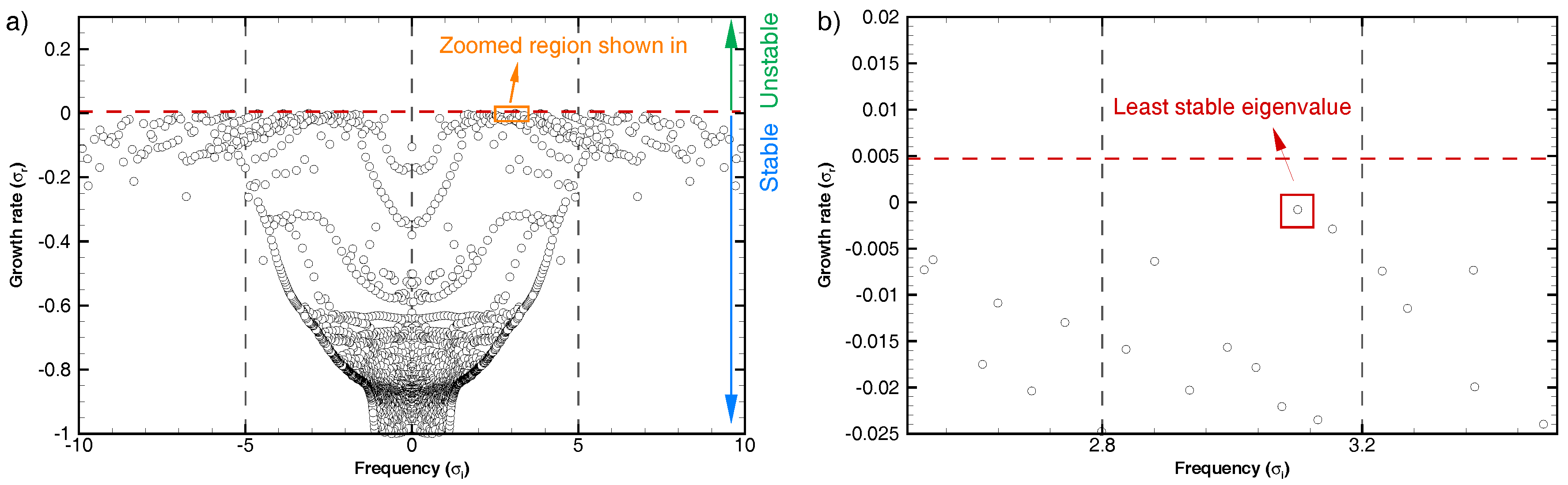
Figure 4.
Contours of instantaneous streamwise velocity (a,b) and vorticity magnitude (c,d). Steady flow shown for Re , in (a,c), and unsteady flow for Re in (b,d). Both flows are computed with the same turbine thrust . Bottom centered (e) depicts the discretised computational domain and the region where the turbine thrust is applied (in red). Zoomed region shows high order mesh.
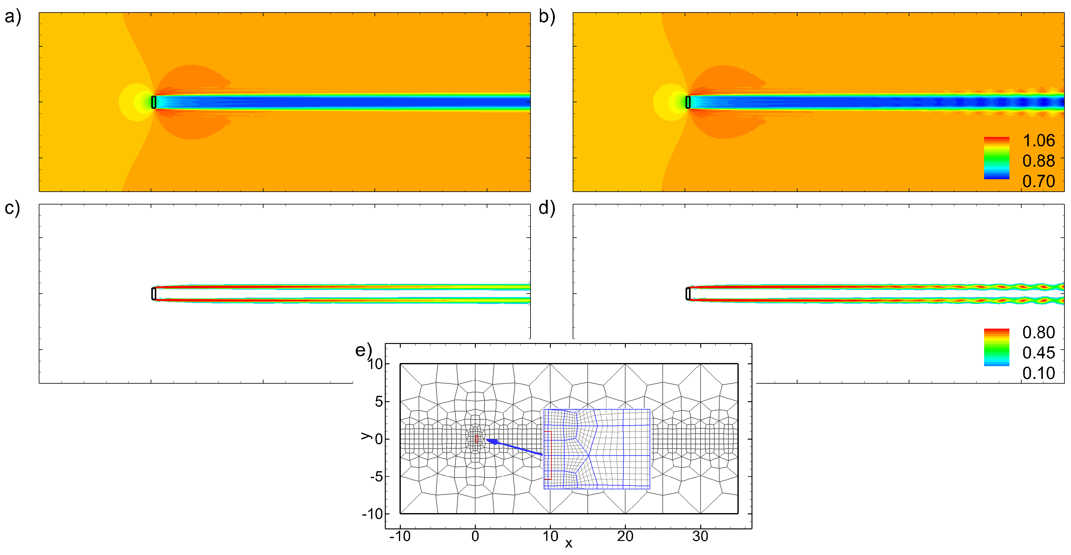
Figure 5.
DG and Ansys-Fluent simulations for : (a,b) show streamwise variation of the non-dimensional static pressure (p) and streamwise velocity () along the domain mid-plane () and (c) shows the velocity deficit downstream of the turbine at . The turbine is marked with red dashed vertical lines. We include inviscid simulations, computations without turbulence model (laminar mode) and using the k-epsilon turbulence model at various Reynolds numbers and turbulence intensities ranging from 0.1% to 10%.
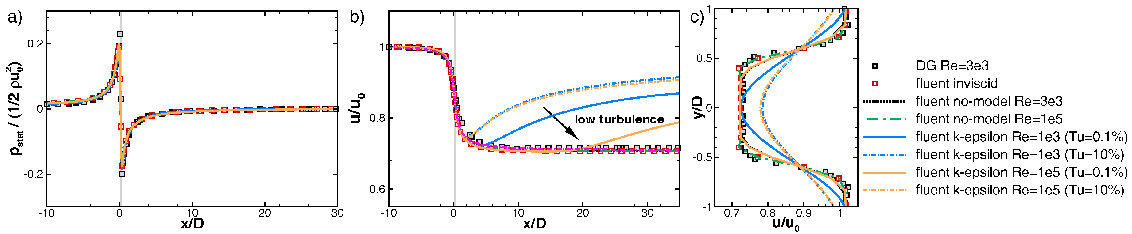
Figure 6.
Streamwise velocity for Re (steady) and 3500 (unsteady), at (a) ; (b) and (c) . Vorticity magnitude along the streamwise line for Re (steady), 3000 (steady), and 3500 (unsteady) are shown in (d).
Figure 6.
Streamwise velocity for Re (steady) and 3500 (unsteady), at (a) ; (b) and (c) . Vorticity magnitude along the streamwise line for Re (steady), 3000 (steady), and 3500 (unsteady) are shown in (d).
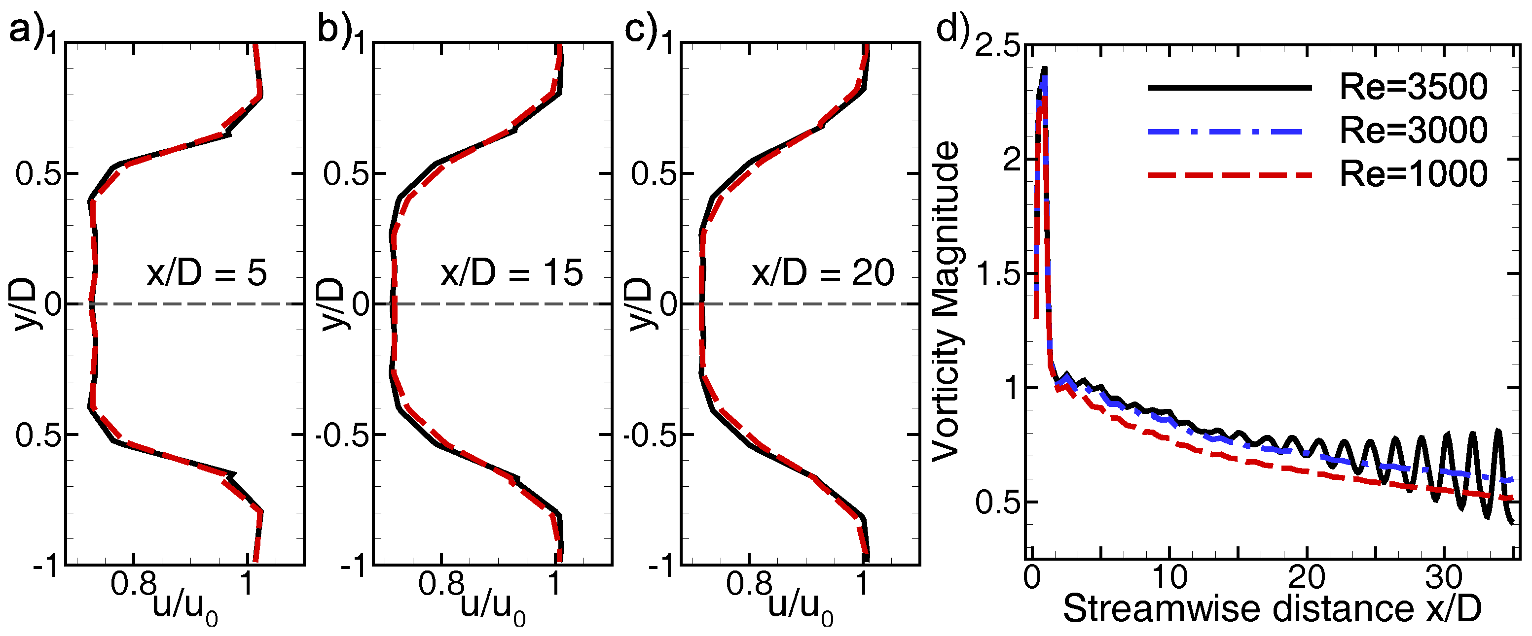
Figure 7.
(a,c) Growth rates for the least stable eigenvalue at various Reynolds numbers (Re) and turbine thrust ; (b,d) frequencies for the least stable eigenvalue at various Reynolds numbers (Re) and turbine thrust .
Figure 7.
(a,c) Growth rates for the least stable eigenvalue at various Reynolds numbers (Re) and turbine thrust ; (b,d) frequencies for the least stable eigenvalue at various Reynolds numbers (Re) and turbine thrust .
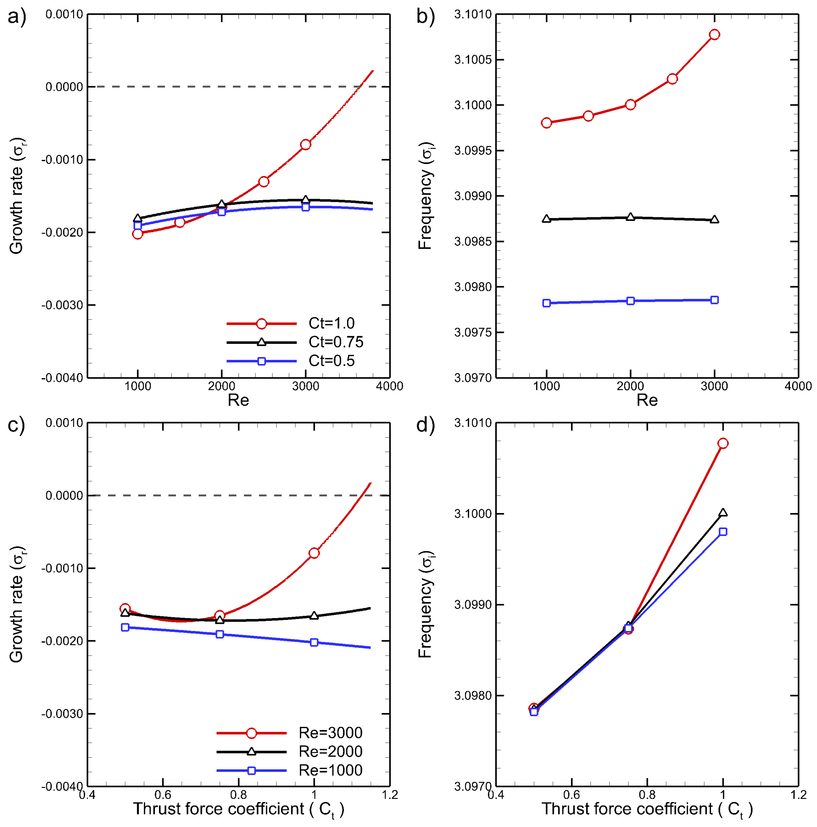
Figure 8.
(a) Direct mode (real part streamwise momentum) and (b) Adjoint mode (real part streamwise momentum), for and (steady case).
Figure 8.
(a) Direct mode (real part streamwise momentum) and (b) Adjoint mode (real part streamwise momentum), for and (steady case).

Figure 9.
Sensitivity of the growth rate to (a) structural sensitivity or wavemaker region; (b) base flow modifications () and (c) a steady force (). Figure (d) shows the positions of pointwise forces to enhance stability: near turbine control (red squares) and downstream control (blue squares). Underlaying in (d) are streamwise velocity contours (gray lines).

Figure 10.
Uncontrolled wake (original) compared to near turbine control () and downstream control (): Growth rates for the least stable eigenvalue for (a) various Reynolds numbers () (fixed turbine thrust ) and (b) various turbine thrusts (and fixed ).
Figure 10.
Uncontrolled wake (original) compared to near turbine control () and downstream control (): Growth rates for the least stable eigenvalue for (a) various Reynolds numbers () (fixed turbine thrust ) and (b) various turbine thrusts (and fixed ).

Figure 11.
Direct mode (real part streamwise momentum) for and for (a) uncontrolled (original); (b) and (c) .
Figure 11.
Direct mode (real part streamwise momentum) for and for (a) uncontrolled (original); (b) and (c) .
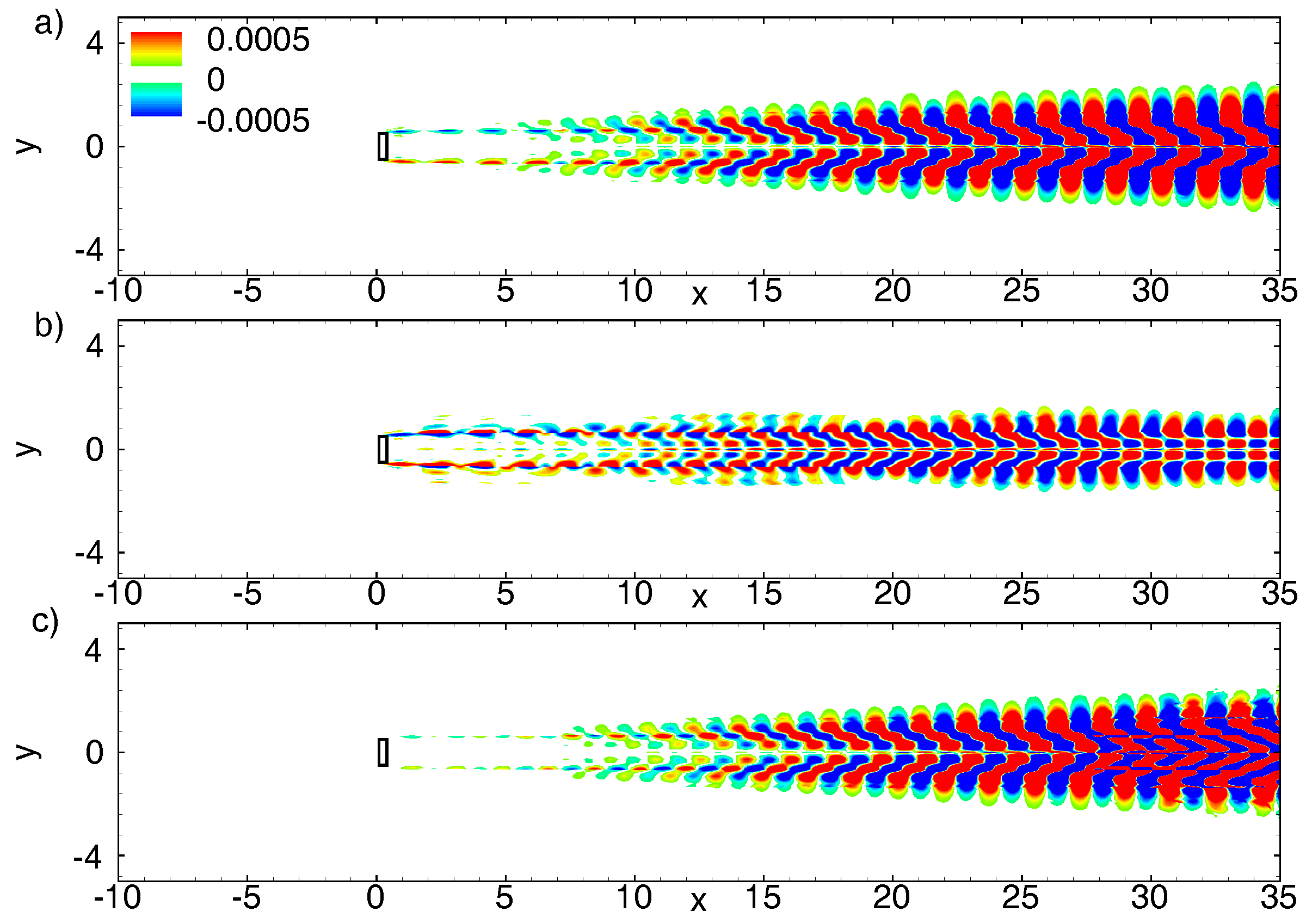
Figure 12.
Uncontrolled wake (original) compared to near turbine control () and downstream control () for and : (a) Vorticity magnitude along the horizontal line and (b) Eigenvalue spectra.
Figure 12.
Uncontrolled wake (original) compared to near turbine control () and downstream control () for and : (a) Vorticity magnitude along the horizontal line and (b) Eigenvalue spectra.

Figure 13.
Streamwise velocity at sections (a): , (b): , (c): , (d): , (e): and (f): . All for and . Results have been interpolated to a homogeneous grid.
Figure 13.
Streamwise velocity at sections (a): , (b): , (c): , (d): , (e): and (f): . All for and . Results have been interpolated to a homogeneous grid.

Figure 14.
Turbulent simulations at Re : (a) Uncontrolled wake and (c) Controlled and stabilised wake; contours of streamwise velocity and velocity streamlines are shown. Zoomed regions of the actuator are depicted in (b,d) for uncontrolled and controlled configurations, respectively. Red boxes in (b,d) show the turbine actuator () and two passive control devices modelled as solid regions.


Table 1.
Convergence of the growth rate () and frequency () with respect to polynomial order. The relative percentage error is defined as % Error .
Table 1.
Convergence of the growth rate () and frequency () with respect to polynomial order. The relative percentage error is defined as % Error .
| P-Order | % Error () | % Error () | ||
|---|---|---|---|---|
| 3 | −0.002287 | 13.611 | 3.0998769 | 0.002 |
| 4 | −0.002019 | 0.298 | 3.099801 | 9.678 × |
| 5 | −0.002013 | - | 3.099798 | - |
Table 2.
Stability of the wake of a turbines when varying the Reynolds number () and the turbine thrust (). The table details the wake behaviour: steady (S) or unsteady (U).
Table 2.
Stability of the wake of a turbines when varying the Reynolds number () and the turbine thrust (). The table details the wake behaviour: steady (S) or unsteady (U).
| Turbine Thrust | Reynolds Number Re | |||||
|---|---|---|---|---|---|---|
| 1000 | 1500 | 2000 | 2500 | 3000 | 3500 | |
| 0.50 | S | S | S | S | S | S |
| 0.75 | S | S | S | S | S | S |
| 1.00 | S | S | S | S | S | U |
| 1.20 | S | S | U | U | U | U |
© 2017 by the authors. Licensee MDPI, Basel, Switzerland. This article is an open access article distributed under the terms and conditions of the Creative Commons Attribution (CC BY) license (http://creativecommons.org/licenses/by/4.0/).
Share and Cite
MDPI and ACS Style
Ferrer, E.; Browne, O.M.F.; Valero, E. Sensitivity Analysis to Control the Far-Wake Unsteadiness Behind Turbines. Energies 2017, 10, 1599. https://doi.org/10.3390/en10101599
AMA Style
Ferrer E, Browne OMF, Valero E. Sensitivity Analysis to Control the Far-Wake Unsteadiness Behind Turbines. Energies. 2017; 10(10):1599. https://doi.org/10.3390/en10101599
Chicago/Turabian StyleFerrer, Esteban, Oliver M.F. Browne, and Eusebio Valero. 2017. "Sensitivity Analysis to Control the Far-Wake Unsteadiness Behind Turbines" Energies 10, no. 10: 1599. https://doi.org/10.3390/en10101599
Note that from the first issue of 2016, this journal uses article numbers instead of page numbers. See further details here.