Short-Circuit Fault Tolerant Control of a Wind Turbine Driven Induction Generator Based on Sliding Mode Observers

Abstract

The installed energy production capacity of wind turbines is growing intensely on a global scale, making the reliability of wind turbine subsystems of greater significance. However, many faults like Inter-Turn Short-Circuit (ITSC) may affect the turbine generator and quickly lead to a decline in supplied power quality. In this framework, this paper proposes a Sliding Mode Observer (SMO)-based Fault Tolerant Control (FTC) scheme for Induction Generator (IG)-based variable-speed grid-connected wind turbines. First, the dynamic models of the wind turbine subsystems were developed. The control schemes were elaborated based on the Maximum Power Point Tracking (MPPT) method and Indirect Rotor Flux Oriented Control (IRFOC) method. The grid control was also established by regulating the active and reactive powers. The performance of the wind turbine system and the stability of injected power to the grid were hence analyzed under both healthy and faulty conditions. The robust developed SMO-based Fault Detection and Isolation (FDI) scheme was proved to be fast and efficient for ITSC detection and localization.Afterwards, SMO were involved in scheming the FTC technique. Accordingly, simulation results assert the efficacy of the proposed ITSC FTC method for variable-speed wind turbines with faulty IG in protecting the subsystems from damage and ensuring continuous connection of the wind turbine to the grid during ITSC faults, hence maintaining power quality.

1. Introduction

Wind energy conversion systems present one of the most safety-critical engineering systems. They include complicated components operating under random wind conditions directly coupled to a constantly varying grid with variable voltages, frequency and power flow. Thus, there is an ever-growing need for security and reliability of the industrial equipment components exposed to potential process anomalies and faults [1]. The faults affecting wind turbine systems can be classified into actuator faults, sensor faults and component faults. Kusiak and Li [2] presented various data-mining algorithms applied to develop models for predicting possible faults affecting wind turbine subsystems. Whatever the kind of the fault, the control action will be interrupted once a fault appears due to the modification of the dynamic properties of the system outputs [3]. This will lead to a degradation of the system performance and even possible damage to the whole system. Hence, to avoid the system collapse and to enhance the reliability, a fault diagnostic scheme is required. Model-based methods represent some of the most successful fault diagnosis methods. These methods are based on availability of the industrial process model generally set up by identification techniques. The fault diagnosis algorithm is implemented to diagnosis the conventionality between measured outputs and predicted ones. Gao et al. [4] reviewed model-based fault diagnosis following the categories of fault diagnosis approaches for deterministic systems, stochastic fault diagnosis methods, discrete-event and hybrid system diagnosis approaches, and networked and distributed system diagnosis techniques, respectively.

Observers represent an important tool able to estimate the system outputs in model-based methods even under faulty conditions. Chen et al. [5] developed diagnostic observer-based approaches using a Kalman filter for residual generation. Sliding Mode Observers (SMOs) have been commonly used in many dynamic systems, like vehicles, robotic, motors, etc. [6]. They represent one of the most robust observers permitting the identification of the type and the shape of faults and furthermore their isolation. This task is called a Fault Detection and Isolation (FDI) scheme. In all diagnostic schemes, FDI is the foremost step. The presence of a fault or malfunction in the conversion system must be quickly detected, as well as its location. Yan and Edwards [7] proved the robustness and the effectiveness of observers based on sliding mode techniques in estimating the system state variables asymptotically, even in the presence of faults. Nonetheless, the FDI scheme is not sufficient. It is a paramount task to implement a Fault Tolerant Control (FTC) algorithm capable of compensating for the degradation of the system performance and especially to protect the equipment. Indeed, a FTC scheme would stabilize the imbalance caused by faults around the nominal equilibrium. Alwi and Edwards [8] implemented an on-line sliding mode control allocation scheme for fault tolerant control and demonstrated the scheme effectiveness in handling failures.

Induction Generators (IG) are frequently used by wind turbine manufacturers thanks to their robustness and low cost. Condition diagnosis of IG is an attractive key to avoid unexpected downtime of variable-speed wind turbines and guarantee a power supply quality. Whether a squirrel cage induction generator (SCIG) or wound rotor induction generator (WRIG) or a doubly fed induction generator (DFIG), the generator can be affected by numerous faults that are typically classified into mechanical and electrical faults. Mechanical faults include essentially gearbox failures, broken rotor bars, bearing failures, air-gap irregularity, etc. The most common electrical faults are open or short circuits in stator or rotor windings (mostly due to winding insulation failures). Each anomaly leads to the interruption of the normal operation of the whole system and requires a proper tolerant action. In this context, this study focuses on Inter-Turn Short-Circuit (ITSC) fault. This fault modifies the system parameters and causes an excessive vibration and abnormal noise [9]. ITSC faults start mostly as unrevealed short circuits of single turns, and then spread over all the turns of the winding. It can lead to an emergency breakdown of the wind turbine system and cut off the connection to the electrical grid. Hence, a fast repair or substitute is required, which is an expensive task.

During starting mode of the wind turbine driven IG, many parameters can deviate from their initial values like IG stator and rotor resistances. However, an ITSC fault is declared when a sudden deviance of one or more of the system characteristic parameters from the standard thresholds occurs. A detailed development of ITSC modelling and its impacts is presented in [10]. Detection of an ITSC fault under system operation conditions is a problematic task and there are currently no efficient industrial solutions. Many solutions have been proposed in the literature to detect and compensate ITSC fault. Isolation testing technique based on the partial discharge analysis was proposed in [11] as a solution for detecting ITSC. Jeong et al. [12] proposed the negative sequence currents analysis approach for diagnosing ITSC faults. In [13], ITSC had also been detected in the field oriented control-based system using the impedance identification. In [14], ITSC faults were detected based on stator resistance estimation by an extended Kalman filter and a Luenberger observer. The Motor Current Signature Analysis (MCSA) technique had been successfully used for detecting ITSC faults [15]. However, the method was applied for open-loop IG-based systems. In this context, this paper proposes stator current estimation by SMO to detect and compensate ITSC faults for closed-loop grid-connected wind turbines.

Some simplifications and assumptions are considered. First, the blades, the tower and the foundation of the system are assumed rigid. Then, as the non-linearity in the aerodynamics of the wind turbine system has to be considered as well as the switching control structure, a static model is used to describe the system aerodynamics. Thus, the developed fault tolerant control scheme is assumed to be robust towards uncertainties in this aerodynamic model.

2. Inter-Turn Short-Circuit (ITSC) Fault Modeling

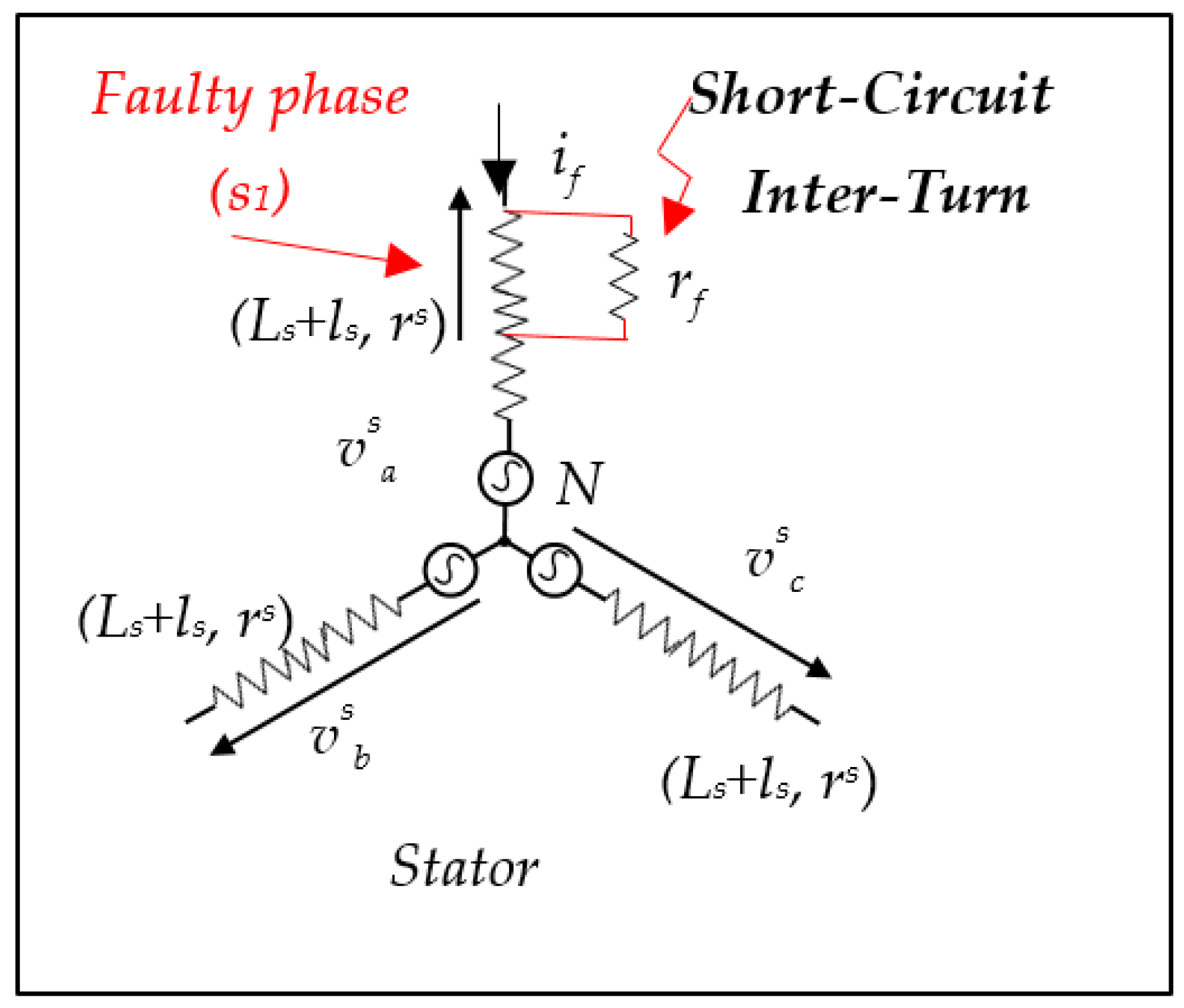
To investigate the effects of short-circuit faults, we consider an IG with an ITSC fault occurring in the first phase s₁ of a stator characterized by a number of turns N^s as presented in Figure 1. The insulation failure in the stator windings caused by the short-circuit fault creates an insulation resistance r_f. A current i_f will then circulate in the line carrying resistance r_f and will determine the severity of the fault. M^s and M^r represent the stator mutual inductances and the rotor mutual inductance, respectively. M_sr presents the mutual inductance between the stator and rotor. The two other phases (s₂ and s₃) resistance r^s and self-inductance L^s are not affected by the fault. As for the rotor scheme, it is also not affected by the fault with a rotor phase resistance r^r and a self-inductance L^r. l^s and l^r present the proper inductance of respectively the stator and the rotor. If N^s_f turns are considered short-circuited, s₁-phase is then divided in to a sub-winding healthy portion (as₁) and a sub-winding faulty portion (bs₁). The factor k_cc can be then defined by dividing N^s_f by N^s (k_cc = N^s_f/N^s). r^s_1b and L^s_1b are considered as resistance and self-inductance of the faulty winding, respectively. The peril of ITSC fault comes from the appearance of M_1a,2 and M_1a,3, the mutual inductances between as₁ and the windings s₂ and s₃, respectively. Additional inductances also appear like M_1a,1b, M_1b,2 and M_1b,3, respectively, created as mutual inductances between bs₁ and as₁, s₂ and s₃, respectively. M_sr1, M_sr2 also appear as mutual inductances between the rotor and as₁ and bs₁, respectively [10].

To study the ITSC fault, it is essential to develop the voltage equations in the (abc)-reference frame [10] as the system is no more considered as an equilibrated three-phase system due to the presence of the harmonic component if. The voltage equations in the (abc)-reference frame are then defined by:

$$\{\begin{array}{l}\left[v^s{}_{abcf}\right]=\left[R^s{}_{abcf}\right]\left[i^s{}_{abc}\right]+\left[L^{ss}{}_{abcf}\right]\frac{d}{dt}\left[i^s{}_{abcf}\right]+\frac{d}{dt}(\left[M^{sr}{}_{abcf}\right]\left[i^r{}_{abc}\right])\\ \left[v^r{}_{abc}\right]=\left[0\right]=\left[R^r{}_{abc}\right]\left[i^r{}_{abc}\right]+\left[L^{rr}{}_{abc}\right]\frac{d}{dt}\left[i^r{}_{abc}\right]+\frac{d}{dt}(\left[M^{rs}{}_{abcf}\right]\left[i^s{}_{abcf}\right])\end{array}$$

(1)

where the system voltage and current vectors are defined by:

$$[v^s{}_{abcf}]={\left[\begin{array}{cccc}{v}^s{}_a& v^s{}_b& v^s{}_c& 0\end{array}\right]}^T, [v^r{}_{abc}]={\left[\begin{array}{ccc}{v}^r{}_a& v^r{}_b& v^r{}_c\end{array}\right]}^T, [i^s{}_{abcf}]={\left[\begin{array}{cccc}{i}^s{}_a& i^s{}_b& i^s{}_c& i_f\end{array}\right]}^T, [i^r{}_{abc}]={\left[\begin{array}{ccc}{i}^r{}_a& i^r{}_b& i^r{}_c\end{array}\right]}^T$$

$\left[R^s{}_{abcf}\right]$, $\left[R^r{}_{abc}\right]$ and $\left[M^{sr}{}_{abcf}\right]$ represent the new parametric stator resistance, rotor resistance and inductance matrices, respectively:

$$\begin{gathered} \left[R^s{}_{abcf}\right]=\left[\begin{array}{cccc}{r}^s& 0& 0& -r_{1b}^s\\ 0& r^s& 0& 0\\ 0& 0& r^s& 0\\ r_{1b}^s& 0& 0& -(r_{1b}^s+r_f)\end{array}\right], \left[R^r{}_{abc}\right]=\left[\begin{array}{ccc}{r}^r& 0& 0\\ 0& r^r& 0\\ 0& 0& r^r\end{array}\right], \\ \left[M^{sr}{}_{abcf}\right]=\left[\begin{array}{ccc}{M}_{sr}\cos (\theta )& M_{sr}\cos (\theta +\frac{2\mathsf{\pi }}{3})& M_{sr}\cos (\theta -\frac{2\mathsf{\pi }}{3})\\ M_{sr}\cos (\theta -\frac{2\mathsf{\pi }}{3})& M_{sr}\cos (\theta )& M_{sr}\cos (\theta +\frac{2\mathsf{\pi }}{3})\\ M_{sr}\cos (\theta +\frac{2\mathsf{\pi }}{3})& M_{sr}\cos (\theta -\frac{2\mathsf{\pi }}{3})& M_{sr}\cos (\theta )\\ -M_{s{r}_2}\cos (\theta )& -M_{s{r}_2}\cos (\theta +\frac{2\mathsf{\pi }}{3})& -M_{s{r}_2}\cos (\theta -\frac{2\mathsf{\pi }}{3})\end{array}\right] \end{gathered}$$

$\left[L^{ss}{}_{abcf}\right]$ and $\left[L^{rr}{}_{abcf}\right]$ represent the stator and rotor new parametric inductance matrices, respectively, defined by:

$$\begin{gathered} \left[L^{ss}{}_{abcf}\right]=\left[\begin{array}{cccc}{L}^s+l^s& M_{1a,2}+M_{1b,2}& M_{1a,3}+M_{1b,3}& -\left(L_{1b}^s+l_{1b}^s+M_{1a,1b}\right)\\ M_{1a,2}+M_{1b,2}& L^s+l^s& M^s& -M_{1b,2}\\ M_{1a,3}+M_{1b,3}& M^s& L^s+l^s& -M_{1b,3}\\ L_{1b}^s+l_{1b}^s+M_{1a,1b}& M_{1a,2}& M_{1a,3}& -\left(L_{1b}^s+l_{1b}^s\right)\end{array}\right], \\ \left[L^{rr}{}_{abc}\right]=\left[\begin{array}{ccc}{L}^r+l^r& M^r& M^r\\ M^r& L^r+l^r& M^r\\ M^r& M^r& L^r+l^r\end{array}\right] \end{gathered}$$

The IG torque equation will be then expressed by:

$$Cem=p(\frac{1}{2}){\left[i_{abcf}\right]}^T\left[\begin{array}{cc}0& \frac{d\left[M^{sr}{}_{abcf}\right]}{d\theta }\\ \frac{d\left[M^{rs}{}_{abcf}\right]}{d\theta }& 0\end{array}\right]\left[i_{abcf}\right]$$

(2)

where $[i_{abcf}]={\left[\begin{array}{ccccccc}{i}^s{}_a& i^s{}_b& i^s{}_c& i_f& i^r{}_a& i^r{}_b& i^r{}_c\end{array}\right]}^T$.

3. Grid-Connected Wind Turbine System Modeling

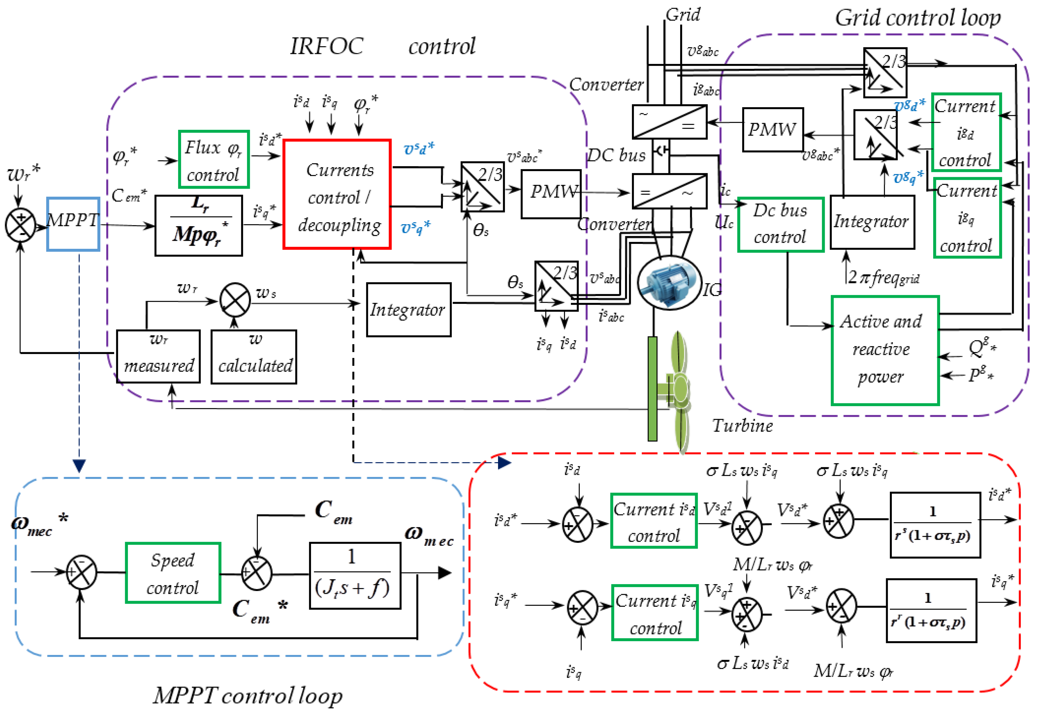
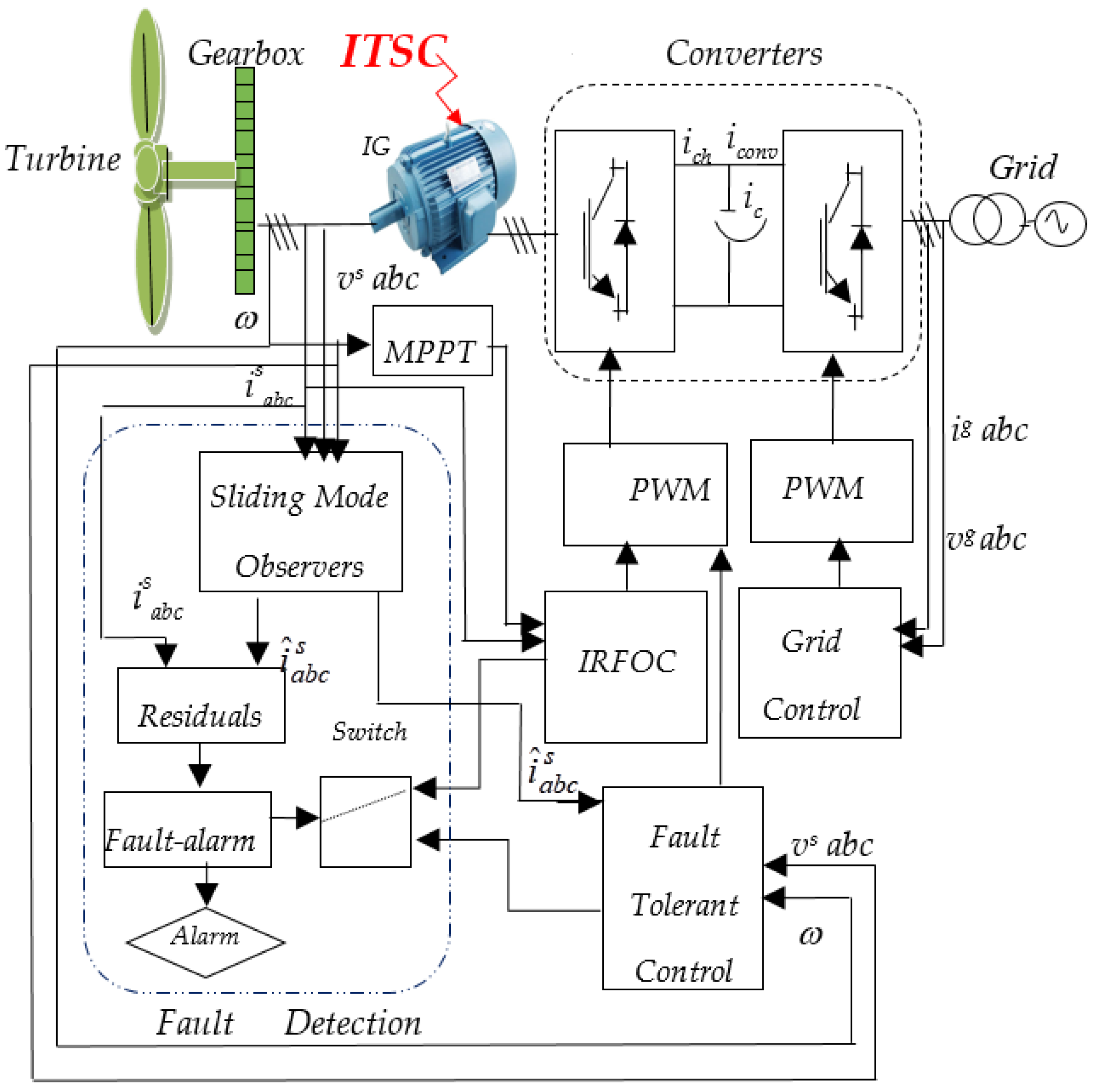
A wind energy conversion system is considered a complex system that comprises subsystems from different physical domains like electrical, mechanical and hydraulic ones. Grid-connected wind turbine system presents a hybrid dynamical system including discrete parts due to presence of power electronic switches (back-to-back converters AC/DC/AC interrelated by a DC bus voltage) and continuous parts (turbine, induction machines, and mechanical drive train). The proposed hybrid system is presented in Figure 2. The cascade control structures are also sketched in the figure with three control loops. A detailed description of the system and control loops will be developed in the following section. In the first loop, a Maximum Power Point Tracking (MPPT) algorithm based on Proportional Integral (PI) controller is used to extract the optimal aerodynamic energy [16]. For a fixed pitch angle β, the loop ensures generating a maximum electromagnetic torque reference. In the second loop, the d, q-axis currents of the generator are controlled by Indirect Rotor Oriented Flux Control (IRFOC) strategy [17]. IRFOC for IG ensures that the system works around the optimal point, which corresponds to the maximum power extracted by the turbine. The third loop is based on regulating the active and reactive grid power according to desired requirements [18]. The control scheme also forces the bus voltage to follow the bus reference. The control loops feed Pulse Width-Modulated (PWM) by three-phase reference voltages that are injected to each converter [19].

3.1. Turbine Modeling and Maximum Power Point Tracking (MPPT) Loop Scheming

The turbine is considered as an inertia mass J_turbine, with a rotor radius R and a power coefficient C_p. C_p is related to the pitch angle β and the tip speed ratio λ. The generator rotor is considered as an inertia mass J_g. The system is characterized by a coefficient of friction relative to the shaft f. A gearbox characterized by a coefficient G, is added to increase the system speed in variable speed turbines. The turbine stores a torque C_ar from the kinetic energy of the wind. The generator rotating at the mechanical speed ω_mec, produces an electromagnetic torque C_em. The turbine is defined by a total inertia J_t expressed by:

$$J_t= \frac{J_{\mathrm{turbine}}}{G^2}+J_g$$

(3)

The mechanical equation of the system is defined by:

$$J_t\frac{d{\omega }_{mec}}{dt}={\mathrm{C}}_{em}-\frac{P_{ar}}{G{\omega }_{mec}}-\mathrm{f}{\omega }_{mec}$$

(4)

P_ar is the absorbed aerodynamic power. ρ is the air density of the air. V is the wind speed.

$$P_{ar}=\frac{1}{2} \rho {\mathsf{\pi }\mathrm{R}}^2 V^3{C}_p\left(\lambda ,\beta \right).$$

(5)

In order to avoid mechanical faults, a pitch angle-control system is generally required in order to limit the speed. When the speed exceeds its nominal value ω_{mec_n}, the blade control system will regulate the pitch angle β. This pitch angle-control loop is described by the following equations:

$$\{\begin{array}{l}{\beta }_{ref}={\beta }_0=0°\hspace{1em}If\hspace{1em}{\omega }_{mec}\le {\omega }_{mec\_n}\\ {\beta }_{ref}=\frac{\mathrm{\Delta }\beta }{\mathrm{\Delta }{\omega }_{mec}}({\omega }_{mec}-{\omega }_{mec}{}_{\_n})\hspace{1em}If\hspace{1em}{\omega }_{mec}\ge {\omega }_{mec\_n}\end{array}$$

(6)

To simulate the dynamics of the angle β, the following first order-transfer function can be introduced by:

$$\beta (s)=\frac{1}{1+{\tau }_{b}s}{\beta }_{ref}$$

(7)

where τ_b is the time constant of the pitch angle system and s is the Laplace operator.

To ensure a maximum of mechanical power is extracted at every instant, a control scheme is required. The MPPT technique is developed under a fixed pitch angle β condition. The loop is based on controlling the rotor speed via PI controllers. Forcing the tip ratio λ to its maximum value λ_opt and the coefficient C_p to its maximum value C_pmax, the electromagnetic reference torque can be expressed by:

$$C_{em}\ast =\frac{V{\lambda }_{opt}}{R}\frac{1}{2} \rho { \mathsf{\pi }\mathrm{R}}^2 V^3{C}_{p\max }$$

(8)

The PI controller defined by K_p (PI controller proportional-parameter controlling the system reply time) and K_i (PI controller integral-parameter controlling the overtaking). The closed-loop transfer function of the system is then calculated by:

$$F(s)= \frac{(k_{p}s+k_i)}{J_t{s}^2+(f+k_p)s+k_i}$$

(9)

Considering the canonical transfer function of two-degree system expressed by:

$$F_0(s)= \frac{K{\omega }_0{}^2}{s^2+2{\omega }_0\xi s+{\omega }_0{}^2}$$

(10)

where ω₀ is the desired natural frequency of the closed-loop system and ξ is the desired damping factor of the closed-loop system. Basing on the identification method with the canonical transfer function of two-degree system [20], the PI controller parameters are then calculated by:

$$\{\begin{array}{l}Ki=J_t{\omega }_0{}^2\\ Kp=\frac{2\xi K_i}{{\omega }_0}-f\end{array}$$

(11)

3.2. IG Modeling and Indirect Rotor Flux Oriented Control (IRFOC) Scheming

The model of the healthy induction machine is defined by considering the resistance r_f and the current i_f absent. Hence, the equilibrium of the system including the three-phase components of both the stator and rotor is established. The IG modeling can be then developed based on transforming the real electrical and mechanical components of respectively the stator and rotor in Park reference frame (d, q) following d (direct axis) and q (quadrature axis):

$$\left[x^s{}_{dq}\right]=\left[P\left({\theta }_p\right)\right]\left[x^s{}_{abc}\right]$$

(12)

$$\left[x^r{}_{dq}\right]=\left[P\left({\theta }_r\right)\right]\left[x^r{}_{abc}\right]$$

(13)

where $\left[P\left({\theta }_p\right)\right]$ is the Park transformation matrix defined by:

$$\left[P\left({\theta }_p\right)\right]=\sqrt{\frac{2}{3}}\left[\begin{array}{ccc}\cos {\theta }_p& \cos \left({\theta }_p-\frac{2\mathsf{\pi }}{3}\right)& \cos \left({\theta }_p-\frac{4\mathsf{\pi }}{3}\right)\\ -\sin {\theta }_p& -\sin \left({\theta }_p-\frac{2\mathsf{\pi }}{3}\right)& -\sin \left({\theta }_p-\frac{4\mathsf{\pi }}{3}\right)\\ \frac{1}{\sqrt{2}}& \frac{1}{\sqrt{2}}& \frac{1}{\sqrt{2}}\end{array}\right]$$

(14)

θ_p is the rotating vector angle. θ_s is the rotating vector angle relative to the stator frame (synchronous speed). θ_r is the rotating vector angle relative to the rotor frame. The speeds ω_p, ω_s and ω_r are defined as the derivative of respectively the angles θ_p, θ_s and θ. ω_r is called the machine electric speed defined by ω = 𝑝ω_mec, where ω_mec is the machine mechanical speed. ϕ^s and ϕ^r are the stator and rotor flux. The IG model is set up in the Park reference frame (d, q) following d (direct axis) and q (quadrature axis). r^r and r^s are the phase resistance of respectively the rotor and the stator of the 𝑝-pairs of poles IG. L_s (stator inductance), L_r (rotor inductance) and M_sr (stator-rotor interaction inductance) are the IG parameters of the machine relative to (d, q)-reference frame. The cyclic mutual inductance between stator and rotor equivalent phases M (M = 3/2 M_sr).

Applying the Park transformation to the stator and rotor voltage, currents and flux equations of the induction machine, the system becomes:

$$\{\begin{array}{l}{v}^s{}_d=r^s{i}^s{}_d+\frac{d{\phi }^s{}_d}{dt}-{\omega }_p{\phi }^s{}_q\\ v^s{}_q=r^s{i}_{sq}+\frac{d{\phi }^s{}_q}{dt}+{\omega }_p{\phi }^s{}_d\\ 0=r^r{i}^r{}_d+\frac{d{\phi }^r{}_d}{dt}-\left({\omega }_p-\omega \right){\phi }^r{}_q\\ 0=r^r{i}^r{}_q+\frac{d{\phi }^r{}_q}{dt}+\left({\omega }_p-\omega \right){\phi }^r{}_d\end{array}$$

(15)

The machine produced electromagnetic torque C_em is expressed by:

$$C_{em}=p\frac{M}{L_r}\left({\phi }^s{}_d{i}^s{}_q-{\phi }^s{}_q{i}^s{}_d\right)$$

(16)

Indirect Rotor Flux Oriented Control (IRFOC) ensures an independent control of both decoupled rotor flux and torque. The scheme controls d and q stator current components based on imposing the rotor flux according to the d-axis (ϕ^r_d = ϕ^r_d and ϕ^r_q = 0) [21]. Using a Laplace transformation of the decoupling equations leads to:

$$\{\begin{array}{l}{v}^s{}_d=(r^s+s\sigma L_s)i^s{}_d+s\frac{M}{L_r}{\phi }_r-{\omega }_s\sigma L_s{i}^s{}_q\\ v^s{}_q=(r^s+s\sigma L_s)i^s{}_q+{\omega }_s\frac{M}{L_r}{\phi }_r+{\omega }_s\sigma L_s{i}^s{}_d\end{array}$$

(17)

The IG control equations are then defined by:

$$\{\begin{array}{l}{\phi }_r=\frac{M}{1+{\tau }_r}{i}^s{}_d\\ C_{em}=p\frac{M}{L_r}{i}^s{}_q\\ {\omega }_r=\frac{M}{{\tau }_r{\phi }_r}{i}^s{}_q\\ {\omega }_s=p{\omega }_{mec}-{\omega }_r\end{array}$$

(18)

To control the rotor flux and the stator currents, PI controllers are required as sketched in Figure 1. Indeed, the imposed flux ϕ_r generates a reference current i^s_d*. The PI controller of the current i^s_d generates a reference voltage v^s_d*. The PI controller of the current i^s_q generates a reference voltage v^s_q*. The speed PI controller, achieved by the MPPT technique, engenders an electromagnetic torque reference C_em*. The parameters of flux and currents PI controllers are chosen using the division compensation technique and according to the desired IG performances (desired damping ratio ξ and natural frequency ω₀) [21]. It is noted that IRFOC scheme controls the stator-side converter. The technique generates three-phase reference voltage v^s_abc* used for Pulse Width-Modulated (PWM) feeding.

3.3. Grid Control Scheme

Considering v^g_d and v^g_q the direct and quadrature components of the grid voltage. The grid currents i^g_d and i^g_q represent the direct and quadrature components. R^g, L^g_d and L^g_q represent the resistance, the direct and quadrature grid inductance, respectively [22]. vⁱ_d and vⁱ_q are the stator-side converter (inverter) voltage components. The dynamic voltages of the grid connection in (d, q)-reference frame are defined by:

$$\{\begin{array}{l}{v}^g{}_d=v^i{}_d-R^g{i}^g{}_d-L^g{}_d\frac{d{i}^g{}_d}{dt}+L^g{}_q{\omega }_g{i}^g{}_q\\ v^g{}_q=v^i{}_q-R^g{i}^g{}_q-L^g{}_q\frac{d{i}^g{}_q}{dt}-L^g{}_d{\omega }_g{i}^g{}_d\end{array}$$

(19)

The DC-link voltage equation is expressed by:

$$C\frac{d{U}_c}{dt}=\frac{3}{2}\frac{v^g{}_d}{U_c}{i}^g{}_d-i_{conv}$$

(20)

U_c is the DC-link voltage and C is the DC-link capacitor. i_conv denotes the transmission line current of the grid side. i_ch is the current circulating in the machine line.

After forcing the grid voltage v^g_q to zero (v^g_q = 0 and v^g_d = v^g), the active and reactive power can be written as:

$$\{\begin{array}{l}{P}^g=\frac{3}{2}{v}^g{}_d{i}^g{}_d\\ Q^g=\frac{3}{2}{v}^g{}_d{i}^g{}_q\end{array}$$

(21)

The active power reference P^g* is calculated based on the grid and DC-bus powers values. A reference of the reactive power is imposed to zero (Q^g* = 0) (A unity power factor). Thus, the references of the active and reactivepowers provide then the reference currents i^g_d*and i^g_q*.

$$\{\begin{array}{l}{i}^g{}_d\ast =\frac{P^g\ast v^g{}_d+Q^g\ast v^g{}_q}{v^g{{}_d}^2+v^g{{}_q}^2}=\frac{P^g\ast }{v^g}\\ i^g{}_q\ast =\frac{P^g\ast v^g{}_q-Q^g\ast v^g{}_d}{v^g{{}_d}^2+v^g{{}_q}^2}=0\end{array}$$

(22)

The grid control scheme based on active-reactive power regulation ensures the adjustment of DC bus voltage and generate the reference voltage v^g_abc*. The grid-side converter is controlled by a PWM supplied by three-phase reference voltages v^g_abc*.

3.4. Wind Turbine System Performance under ITSC Faulty Conditions

The purpose of this section is to present the ITSC fault impact on the performance of the wind turbine system. Thus, simulations are realized using MATLAB/SIMULINK (2013, Natick, MA, USA) environment. The tested grid-connected wind turbine system is characterized by a 14 m-radius turbine. The turbine parameters are λ_opt = 5 and C_pmax = 0.44. It is connected to 11 kW IG rotating with 1450 tr/min nominal speed. The tested IG is a machine of 4-poles, 50 Hz frequency and 380/660 V voltage. The IG load current is i^s₀ = 4 A and the rated current i^s_n = 11.32 A. It is characterized by a stator turns number N^s = 48 and rotor turns number N^r = 32. The stator resistance r^s and inductance L^s are respectively 1.5 Ω and 0.28 H. The rotor resistance r^r and inductance L^r are respectively 0.7 Ω and 0.28 H.

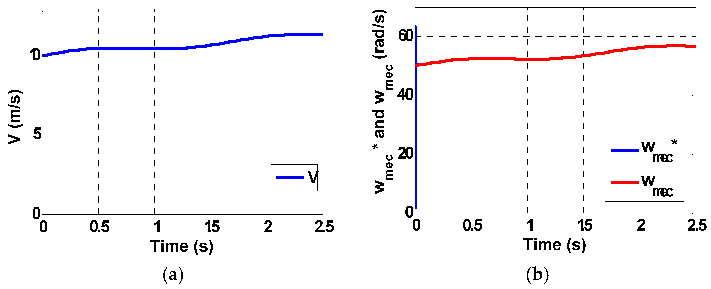
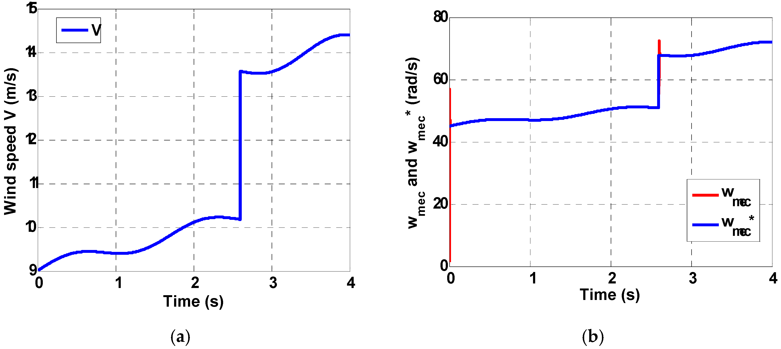
The nominal wind speed of the tested turbine is 10 m/s. We have applied a variable profile of wind in such a way that the wind speed stays between the cut-in and the cutout speeds in order to focus on the ITSC fault impact. The pitch angle β is considered constant and equal to β₀. Figure 3 shows the applied wind speed profile over a period of 2.5 s. The MPPT loop forces the mechanical speed ω_mec to follow the calculated reference speed ω_mec* as presented in Figure 3b.

First, no short-circuited turns are presented. Then, at the instant t = 1.5 s, ITSC fault is introduced. In fact, 30% of the turns of the first phase (s₁) are short-circuited (k_cc = 0.3). r_f was fixed to 0 Ω due to the quick decrease of this insulation resistance r_f in most machine materials. All the components of the subsystems are disturbed reflecting the stator fault effects.

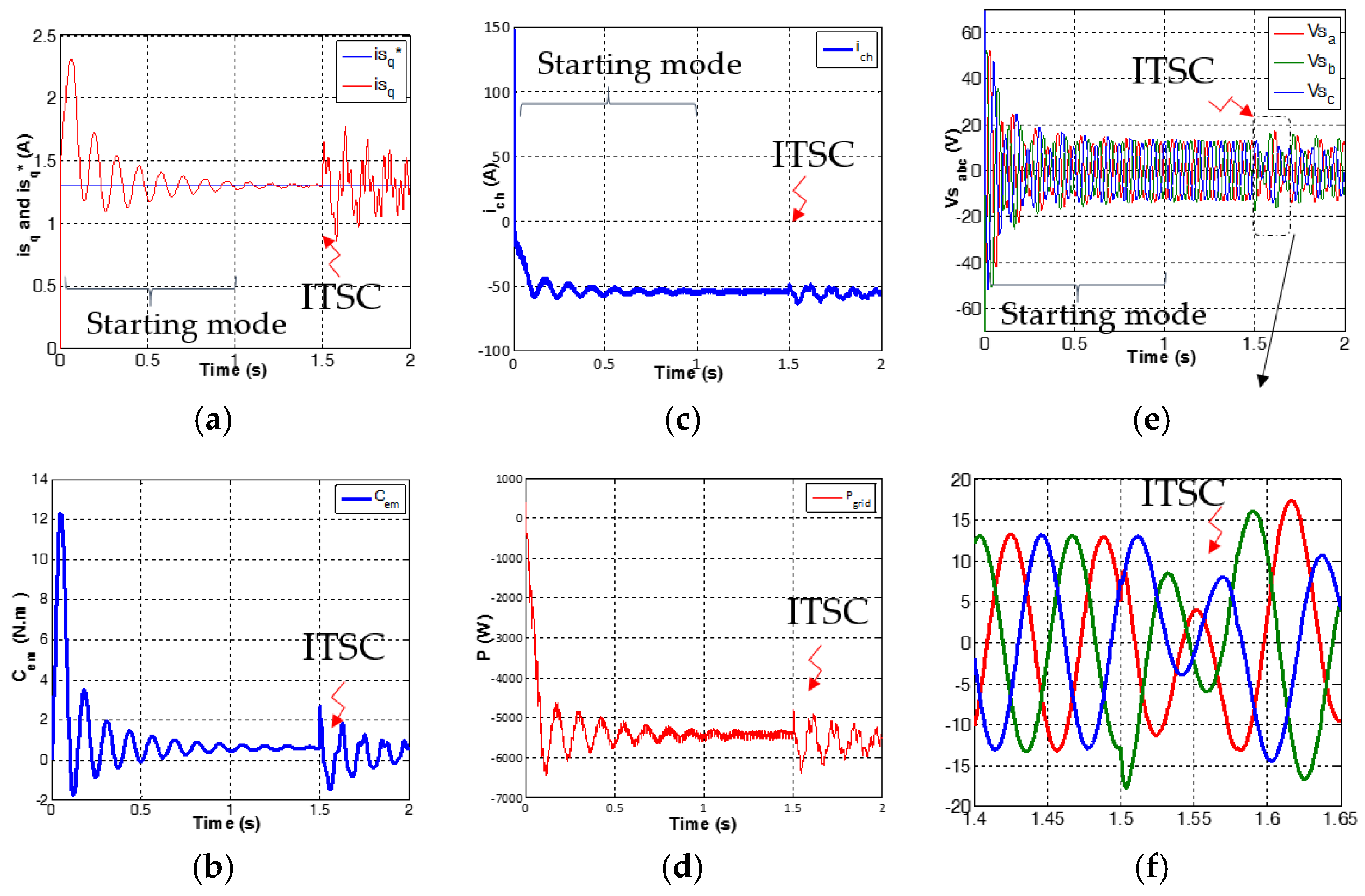
Time-domain signatures analysis is a good tool for evaluating ITSC fault impacts. Figure 4 presents the simulation results in time-domain of the outputs signals of the studied control schemes the most disturbed by ITSC fault. The currents control of stator current i^s_q and its reference i^s_q* are presented by Figure 4a while applying the ITSC fault at t = 1.5 s. It can be observed that important oscillations of the IRFOC-based controlled current i^s_q are presented after the appearance of the fault. It is noted that the aim of the system control schemes is to ensure the stability between the system components. However, the fluctuations of the IG electromagnetic torque C_em presented in Figure 4b are reflected on the stator-side converter output current i_ch (Figure 4c). Figure 4d shows that instability oscillations are reflected in the power quality delivered to the grid. It can be deducted that the fault affects directly the stability of the grid-connection equipment starting with stator-side converter. As a result, the injected power to the grid P^g is disturbed.

Figure 4e,f present the IRFOC outputs, which are the supplied stator three-phase voltages (v^s_a, v^s_b and v^s_c). It is seen that, the stator voltages are balanced under healthy conditions ([0...1.5 s] interval). However, once ITSC fault takes a place, an unbalance appears. The magnitude of the stator faulty voltage v^s_a decreases. The magnitude of the two-phase voltages (v^s_b and v^s_c) increase. These imbalanced voltages (v^s_a, v^s_b and v^s_c) present the implicit cause of the instability of the system power supplied to grid. Thus, IRFOC scheme must to be replaced by a robust fault tolerant control technique able to compensate ITSC influences.

4. Inter-Turn Short-Circuit Fault Detection and Tolerant Control

The purpose of this section is to develop an active Fault Tolerant Control (FTC) scheme ensuring the stability of the wind turbine system with acceptable performance under ITSC fault conditions. Figure 5 presents the diagram block of the developed FTC technique. In the proposed strategy, a Fault Detection and Isolation (FDI) block is first designed to detect and isolate ITSC faulta. Alarm signals are then triggered declaring the fault presence and identifying the faulty phase. In fact, the observed fluctuations in the three-phase stator currents are adopted in residuals generation based on sliding mode observers. Then, the comparison between the residuals and their correspondent thresholds will allow detecting and isolating the ITSC fault. Afterwards, the FDI block outputs are involved in the reconfiguration of a control law for compensating the ITSC fault impact and protecting the equipment. Henceforward, the proposed control law, named FTC scheme, is developed in order to minimize the deviation of the state components from their reference values under faulty conditions.

4.1. Sliding Mode Observers (SMO) Development

The goal of this section is to develop Sliding Mode Observers (SMO) in order to detect and isolate the ITSC fault in a first step and to compensate the ITSC fault impacts in a second step [23]. SMO, involved in both FDI and FTC schemes, predict the stator currents under faulty conditions thanks to Lyapunov theory [24]. The system equations are developed in stator (αβ)-stationary reference using Park transformation matrix ([P(θ_p] = 0).Basing on the five-order nonlinear system of the IG in the (αβ)-reference frame, the equations of SMO-based system are defined by:

$$\{\begin{array}{l}\left[{\widehat{X}}^{\prime }\right]=\left[A\right]\left[\widehat{X}\right]+\left[B\right]\left[\widehat{U}\right]+\lambda \mathrm{sgn}(S_i)\\ \left[\widehat{Y}\right]=\left[C\right][\widehat{X}]\end{array}$$

(23)

where the input, output and state vectors are defined by:

$$\left[U\right]={\left[\begin{array}{cc}{v}^s{}_{\alpha }& v^s{}_{\beta }\end{array}\right]}^T, [Y]={\left[\begin{array}{cc}{i}^s{}_{\alpha }& i^s{}_{\beta }\end{array}\right]}^T, [X]={\left[\begin{array}{cccc}{i}^s{}_{\alpha }& i^s{}_{\beta }& {\phi }^r{}_a& {\phi }^r{}_{\beta }\end{array}\right]}^T$$

The matrices A, B and C are defined as follows:

$$A=\left[\begin{array}{cccc}-a_1& 0& a_3& a_2\omega \\ 0& -a_1& -a_2\omega & a_3\\ a_5& 0& -a_4& -\omega \\ 0& a_5& \omega & -a_4\end{array}\right], B=\left[\begin{array}{cc}b& 0\\ 0& b\\ 0& 0\\ 0& 0\end{array}\right], C=\left[\begin{array}{cccc}1& 0& 0& 0\\ 0& 1& 0& 0\end{array}\right]$$

where a_i (i = 1, ..., 8) and b are the system parameters defined by:

$$a_1=(\frac{1}{\sigma {\tau }_s}+\frac{1-\sigma }{\sigma {\tau }_r}), a_2=\frac{1-\sigma }{\sigma M_{sr}}, a_3=\frac{1-\sigma }{\sigma M_{sr}{\tau }_r}, a_4=\frac{1}{{\tau }_r}, a_5=\frac{M_{sr}}{{\tau }_r}, a_6=\frac{P^2{M}_{sr}}{J_g{L}_r}, a_7=\frac{f}{J_g}, a_8=\frac{P}{J_g}, b=\frac{1}{\sigma L_s}, \sigma =1-\frac{M_{sr}{}^2}{L_s{L}_r}, {\tau }_s=\frac{L_s}{r^s}, {\tau }_r=\frac{L_r}{r^r}$$

The unknown parametric vector λ (λ = [λ₁, λ₂, λ₃, λ₄]^T) is defined with [λ₁] = [λ₁₁ λ₁₂], [λ₂] = [λ₂₁ λ₂₂], [λ₃] = [λ₃₁ λ₃₂] and [λ₁] = [λ₄₁ λ₄₂]. To estimate the stator currents and rotor flux dynamics errors, estimated errors e_i (i = 1, ..., 4) are defined by:

$$\{\begin{array}{l}{e}_1=i^s{}_{\alpha }-{\widehat{i}}_{\alpha }^s\\ e_2=i^s{}_{\beta }-{\widehat{i}}_{\beta }^s\\ e_3={\phi }^r{}_{\alpha }-{\widehat{\phi }}_{\alpha }^r\\ e_4={\phi }^r{}_{\beta }-{\widehat{\phi }}_{\beta }^r\end{array}$$

(24)

S_i (i = 1, 2) carry the difference between measured and estimated stator currents. This choice is due to the possibility of measurement of currents and the slowness of the speed. S_i (i = 1, 2) is then defined by:

$$\{\begin{array}{l}{S}_1=e_1=i^s{}_{\alpha }-{\widehat{i}}_{\alpha }^s\\ S_2=e_1=i^s{}_{\beta }-{\widehat{i}}_{\beta }^s\end{array}$$

(25)

The dynamic of the observer errors can then be expressed by:

$$\left[\begin{array}{c}{\dot{e}}_1\\ {\dot{e}}_2\\ {\dot{e}}_3\\ {\dot{e}}_4\end{array}\right]=\left[\begin{array}{cccc}-a_1& 0& a_3& a_2\omega \\ 0& -a_1& -a_2\omega & a_3\\ a_5& 0& -a_4& -\omega \\ 0& a_5& \omega & -a_4\end{array}\right]\left[\begin{array}{c}{e}_1\\ e_2\\ e_3\\ e_4\end{array}\right]-\left[\begin{array}{cc}{\lambda }_{11}& {\lambda }_{12}\\ {\lambda }_{21}& {\lambda }_{22}\\ {\lambda }_{31}& {\lambda }_{32}\\ {\lambda }_{41}& {\lambda }_{42}\end{array}\right]\left[\begin{array}{c}\mathrm{sgn}(S_1)\\ \mathrm{sgn}(S_2)\end{array}\right]$$

(26)

Lyapunov condition imposes the following equation:

$$V=\frac{S^{T}S}{2}$$

(27)

Defining then the sliding surface S by:

$$S=\left[\begin{array}{c}{S}_1\\ S_2\end{array}\right]=Q\left[\begin{array}{c}{e}_1\\ e_2\end{array}\right]$$

(28)

where Q is a regular matrix. When $S=0$ we get $e_1=0$ and $e_2=0$. Thus, the derivative of the Lyapunov function is expressed by:

$$\dot{V}=S^{T}Q\left[\begin{array}{c}{\dot{e}}_1\\ {\dot{e}}_2\end{array}\right]+S^T\dot{Q}\left[\begin{array}{c}{e}_1\\ e_2\end{array}\right]$$

(29)

Replacing ${\dot{e}}_1$ and ${\dot{e}}_2$ by their expression, we get:

$$\dot{V}=S^{T}Q\left(\left[\begin{array}{cc}{a}_3& a_2\omega \\ -a_2\omega & a_3\end{array}\right]\left[\begin{array}{c}{e}_3\\ e_4\end{array}\right]-\left[\begin{array}{cc}{\lambda }_{11}& {\lambda }_{12}\\ {\lambda }_{31}& {\lambda }_{32}\end{array}\right]\left[\begin{array}{c}\mathrm{sgn}(S_1)\\ \mathrm{sgn}(S_2)\end{array}\right]\right)+S^T\dot{Q}\left[\begin{array}{c}{e}_1\\ e_2\end{array}\right]$$

(30)

Supposing that:

$$Q^{-1}=\left[\begin{array}{cc}{a}_3& a_2\omega \\ -a_2\omega & a_3\end{array}\right],\left[\begin{array}{cc}{\lambda }_{11}& {\lambda }_{12}\\ {\lambda }_{31}& {\lambda }_{32}\end{array}\right]=Q^{-1}\left[\begin{array}{cc}{\gamma }_1& 0\\ 0& {\gamma }_2\end{array}\right]$$

The derivative of Lyapunov function becomes:

$$\dot{V}=S_1(e_3-{\gamma }_1.\mathrm{sgn}(S_1))+S_2(e_4-{\gamma }_2\mathrm{sgn}(S_2))+S^T\dot{Q}\left[\begin{array}{c}{e}_1\\ e_2\end{array}\right]$$

(31)

Taken in to account the slowness of the speed ω, then $\dot{Q}$ is close to zero. The attractive condition is imposed then:

$$\{\begin{array}{l}{S}_1(e_3-{\gamma }_1.\mathrm{sgn}(S_1))<0\\ S_2(e_4-{\gamma }_2\mathrm{sgn}(S_2)>0\end{array}$$

(32)

If we select ${\gamma }_1$ and ${\gamma }_2$ verifying ${\gamma }_1>{\left|e_3\right|}_{\max }$ and ${\gamma }_2>{\left|e_4\right|}_{\max }$ where ${\left|e_3\right|}_{\max }$ and ${\left|e_4\right|}_{\max }$ denote the maximums values of e₃ and e₄, after a finite time, the convergence to the surface $S={\left[\begin{array}{cc}{S}_1& S_2\end{array}\right]}^T$ is got. Then, the dynamic of e₃ and e₄ of can be expressed by:

$$\left[\begin{array}{c}0\\ 0\end{array}\right]=Q^{-1}\left(\left[\begin{array}{c}{e}_3\\ e_4\end{array}\right]-\left[\begin{array}{cc}{\gamma }_1& 0\\ 0& {\gamma }_2\end{array}\right]\left[\begin{array}{c}\mathrm{sgn}(S_1)\\ \mathrm{sgn}(S_2)\end{array}\right]\right)$$

(33)

Using the Filipov method, the vector « sgn » can be defined by:

$$I_s=\left[\begin{array}{c}\mathrm{sgn}(S_1)\\ \mathrm{sgn}(S_2)\end{array}\right]={\left[\begin{array}{cc}\frac{e_3}{{\gamma }_1}& \frac{e_4}{{\gamma }_2}\end{array}\right]}^T$$

(34)

After replacing sgn(S₁) and sgn(S₂) by their expressions, the dynamic of errors becomes:

$$\left[\begin{array}{c}{\dot{e}}_3\\ {\dot{e}}_4\end{array}\right]=\left(-\left[\begin{array}{cc}{\lambda }_{21}& {\lambda }_{22}\\ {\lambda }_{41}& {\lambda }_{42}\end{array}\right]\left[\begin{array}{cc}\frac{1}{{\gamma }_1}& 0\\ 0& \frac{1}{{\gamma }_2}\end{array}\right]\right)\left[\begin{array}{c}{e}_3\\ e_4\end{array}\right]$$

(35)

It can be then selected:

$$\left[\begin{array}{cc}{\lambda }_{21}& {\lambda }_{22}\\ {\lambda }_{41}& {\lambda }_{42}\end{array}\right]=\left[\begin{array}{cc}{q}_1& 0\\ 0& q_2\end{array}\right]\left[\begin{array}{cc}{\gamma }_1& 0\\ 0& {\gamma }_2\end{array}\right]$$

(36)

Basing on the stability condition [10], the parametric vector λ_i (i = 1, …, 4) can be calculated by:

$$\{\begin{array}{l}{\lambda }_1=\left[\begin{array}{cc}{a}_2.{\gamma }_1& a_3.\omega .{\gamma }_2\end{array}\right]\\ {\lambda }_2=\left[\begin{array}{cc}{q}_1{\gamma }_1& 0\end{array}\right]\\ {\lambda }_3=\left[\begin{array}{cc}-a_3.\omega .{\gamma }_1& a_2.{\gamma }_2\end{array}\right]\\ {\lambda }_4=\left[\begin{array}{cc}0& q_2{\gamma }_2\end{array}\right]\end{array}$$

(37)

The reconstructed three-phase current i^s_abc in the (abc)-real frame is then established using Park matrix transformation.

$$\left[{\widehat{i}}_{abc}^s\right]=\left[P\left({\theta }_p=0\right)\right]\left[{\widehat{i}}_{\alpha \beta }^s\right]$$

(38)

4.2. ITSC Fault Detection and Isolation (FDI) Scheming

The basic idea of observer-based diagnostic methods is to generate residuals that are close to zero under healthy conditions. Then they deviate from zero under faulty conditions [18]. When the residuals exceed thresholds, an alarm is triggered to indicate the detection of the fault.

The thresholds of the IG currents are calculated according to the healthy boundary parametric variations of the tested machine. Tis_a, Tis_b and Tis_c present the three thresholds for respectively the three stator currents i^s_a, i^s_b and i^s_c. Their corresponding residuals are respectively Ris_a, Ris_b and Risc. The expressions of residuals relative to the IG stator currents are defined by:

$$\{\begin{array}{l}R i{s}_a=i^s{}_a-{\widehat{i}}_a^s\\ R i{s}_b=i^s{}_b-{\widehat{i}}_b^s\\ R i{s}_c=i^s{}_c-{\widehat{i}}_c^s\end{array}$$

(39)

The overtaking of residuals (Ris_a__max, Ris_b__bmax and Ris_c__max) is cached by a fault-alarm signal FD as follows:

• - FD = 1 if Ris_{k_max (k = a, b, c)} > Tis_{k (k = a, b, c)} (the fault is declared),
• - FD = 0 if Ris_{k_max (k = a, b, c)} < Tis_{k (k = a, b, c)} (no fault is declared).

The last phase of the FDI scheme is the isolation of the faulty phase. Thus, three fault-alarm signals FI1, FI2 and FI3 are defined. The ITSC fault isolation scheme is given by the following algorithm:

• - FI1 = 1, FI2 = 0 and FI3 = 0 if Ris_{a_max} = max (Ris_{a_max}, Ris_{b_max}, Ris_{c_max}),
• - FI2 = 1, FI1 = 0 and FI3 = 0 if Ris_{b_max} = max (Ris_{a_max}, Ris_{b_max}, Ris_{c_max}),
• - FI3 = 1, FI2 = 0 and FI1 = 0 if Ris_{c_max} = max (Ris_{a_max}, Ris_{b_max}, Ris_{c_max}).

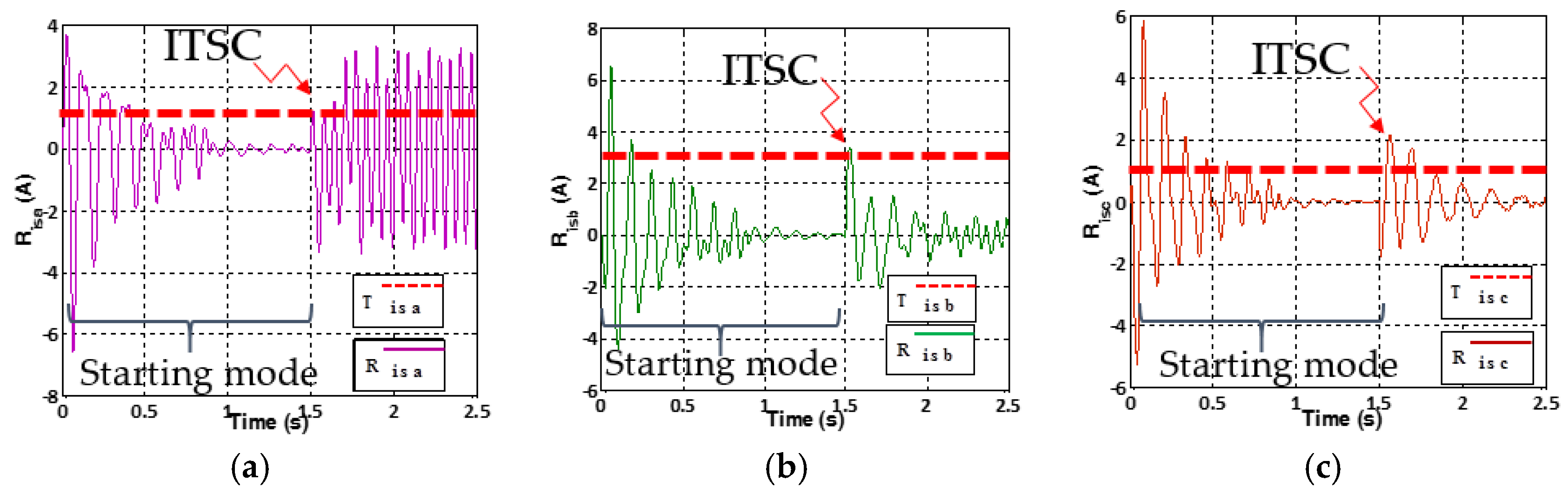
Simulations are now developed with the SMO implementation. At the instant t = 1.5 s, an ITSC fault is introduced (30% of the turns of the first phase (s₁) are short-circuited (k_cc = 0.3 and r_f = 0 Ω)). The pitch angle β is maintained constant and equal to β₀. The currents residuals and their corresponding thresholds Tis_a, Tis_b and Tis_c are collected in Figure 6. Tis_a, Tis_b and Tis_c magnitudes of the 11KW-IG under test are fixed to 1 A based on simulation results under healthy conditions and operating resistance variations. The IG operates in the starting mode until 1 s. Thus, the FDI method takes 1 s to operate until the residuals stability. It can be seen that the residuals exceed the thresholds at t = 1.6 s because of the fault presence. The fault alarm signal FD changes then from 0 to 1.

The highest magnitude of fault-alarm signals corresponds to the stator phase affected by the ITSC. Thus, only the fault-alarm signal FI1 deviates from 0 to 1 (FI1 = 1, FI2 = 0 and FI3 = 0) as Ris_{a_max} = max (Ris_{a_max}, Ris_{b_max}, Ris_{c_max}). FI1 declares that the first phase (s₁) is suffering from an ITSC fault.

4.3. Fault Tolerant Control (FTC) Strategy Scheming

The idea of the proposed FTC scheme is to regulate the control input under faulty conditions by replacing the measured stator currents by the SMO-reconstructed ones [25,26,27]. The control law can be expressed by:

$$\{\begin{array}{l}{v}^s{}_d=(r^s+s\sigma L_s){\widehat{i}}_d^s+s\frac{M}{L_r}{\phi }_r-{\omega }_s\sigma L_s{\widehat{i}}_q^s\\ v^s{}_q=(r^s+s\sigma L_s){\widehat{i}}_q^s+{\omega }_s\frac{M}{L_r}{\phi }_r+{\omega }_s\sigma L_s{\widehat{i}}_d^s\\ C_{em}=p\frac{M}{L_r}\left({\phi }^s{}_d{\widehat{i}}_q^s-{\phi }^s{}_q{\widehat{i}}_d^s\right)\end{array}$$

(40)

where ${\widehat{i}}_d^s$ and ${\widehat{i}}_q^s$ are the SMO estimated currents in (d, q)-reference frame.

In this context, the proposed FTC approach could be summarized by:

-

Under healthy conditions (FDI declares the ITSC absence), the IRFOC is adopted to calculate the voltages and the torque v^s_d, v^s_q and C_em basing on the measured stator current i^s_d and i^s_q.

-

Under faulty conditions (FDI declares the ITSC presence), the FTC is adopted to calculate the voltages and the torque v^s_d, v^s_q and C_em basing on the SMO reconfigured stator current ${\widehat{i}}_d^s$ and ${\widehat{i}}_q^s$.

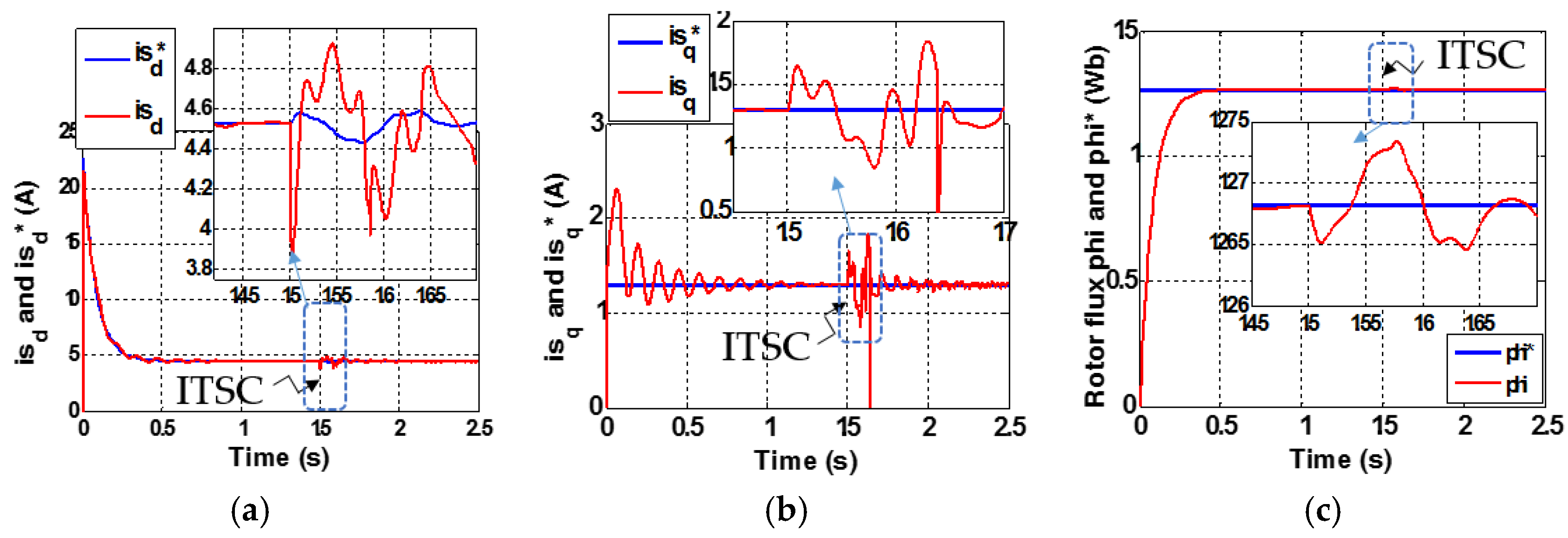
Figure 7 presents the simulation results of the control signals of the proposed FTC technique while applying the ITSC fault at t = 1.5 s. The control of stator currents (i^s_d, i^s_q) and their references (i^s_d*, i^s_q*) are represented by Figure 7a,b, respectively. Figure 7c represents the rotor flux (ϕ_r) and its reference elaborated by the FTC method. It can be seen that fluctuations appear in the control outputs once the fault is present. Indeed, short-circuit fault leads to a significant instability at the instant of the occurrence of the fault. However, SMO reconfigure the stator currents allowing the FTC technique to compensate the fault impacts. Hence, the system carries on operating with an acceptable yield despite the presence of ITSC fault.

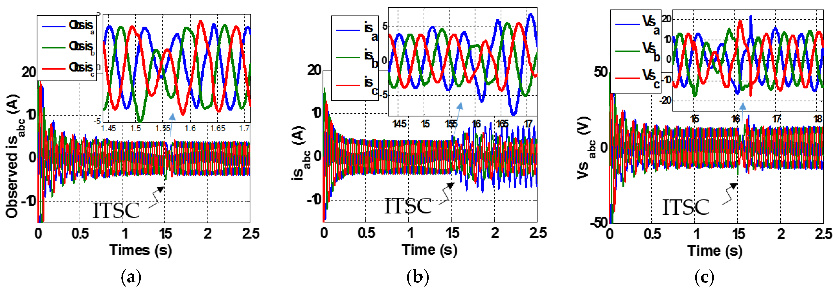
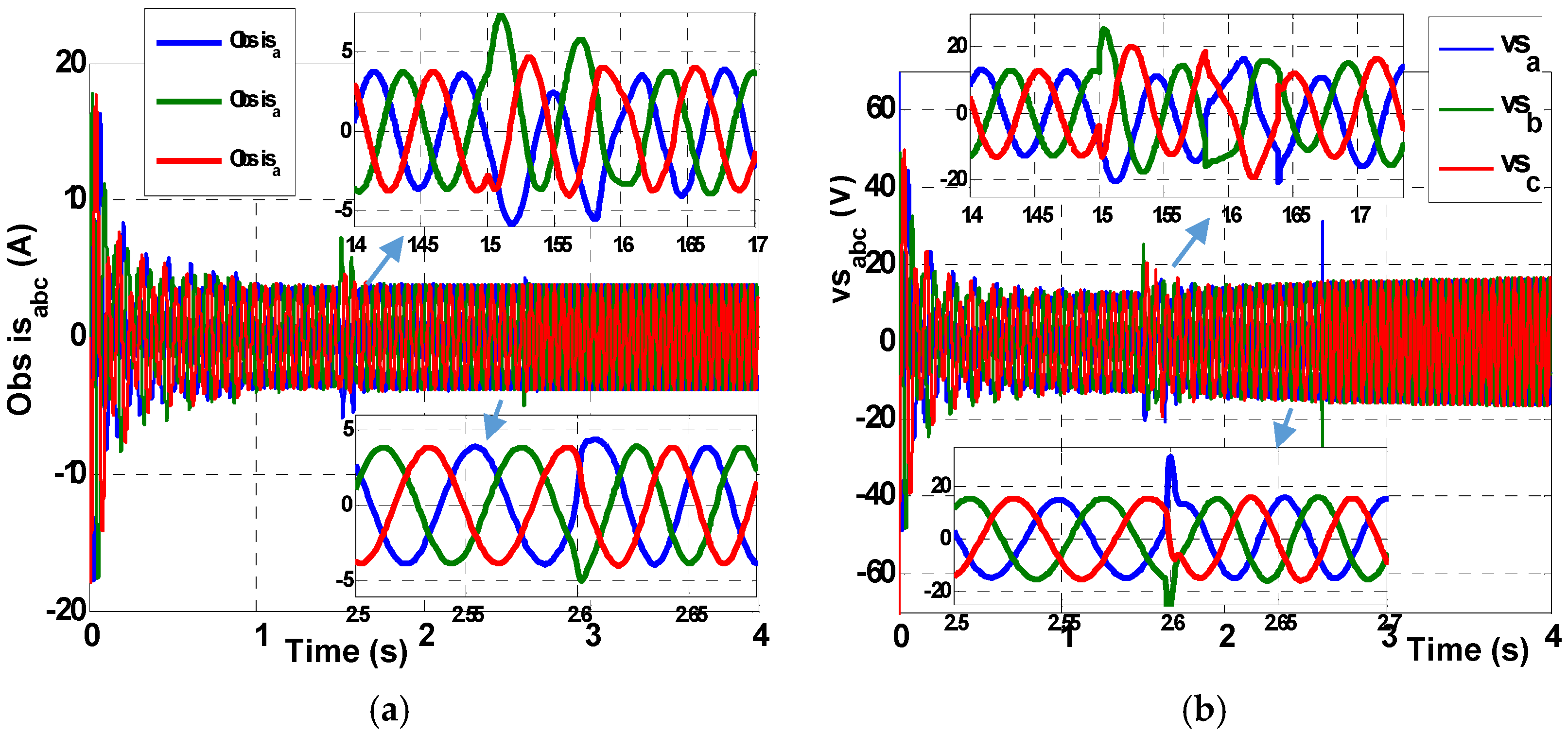
The reconstructed three-phase currents (${\widehat{i}}_a^s$, ${\widehat{i}}_b^s$ and ${\widehat{i}}_c^s$) by SMO are presented in Figure 8a. The measured three-phase stator currents i^s_abc are presented in Figure 8b. Comparing the measured and SMO-observed currents, it can be noticed that at the instant of appearance of the ITSC fault, the three reconstructed currents start to be imbalanced just like measured ones. Then, the SMO restore the equilibrium after 0.2 s (at t = 1.7 s). It can be then deducted that SMO are able to compensate ITSC fault impacts and reconstruct quickly three-phase stator currents insensitive to the fault presence. The reconstructed currents allow generating adequate inputs to the FTC block. Figure 8c presents the supplied stator three-phase voltages (v^s_a, v^s_b and v^s_c) that present the FTC block outputs. It is noticed that, the stator voltages are balanced under healthy conditions ([0...1.5 s] interval). Once ITSC fault takes a place, an unbalance appears. The FTC scheme returns them to balance.

5. Discussion

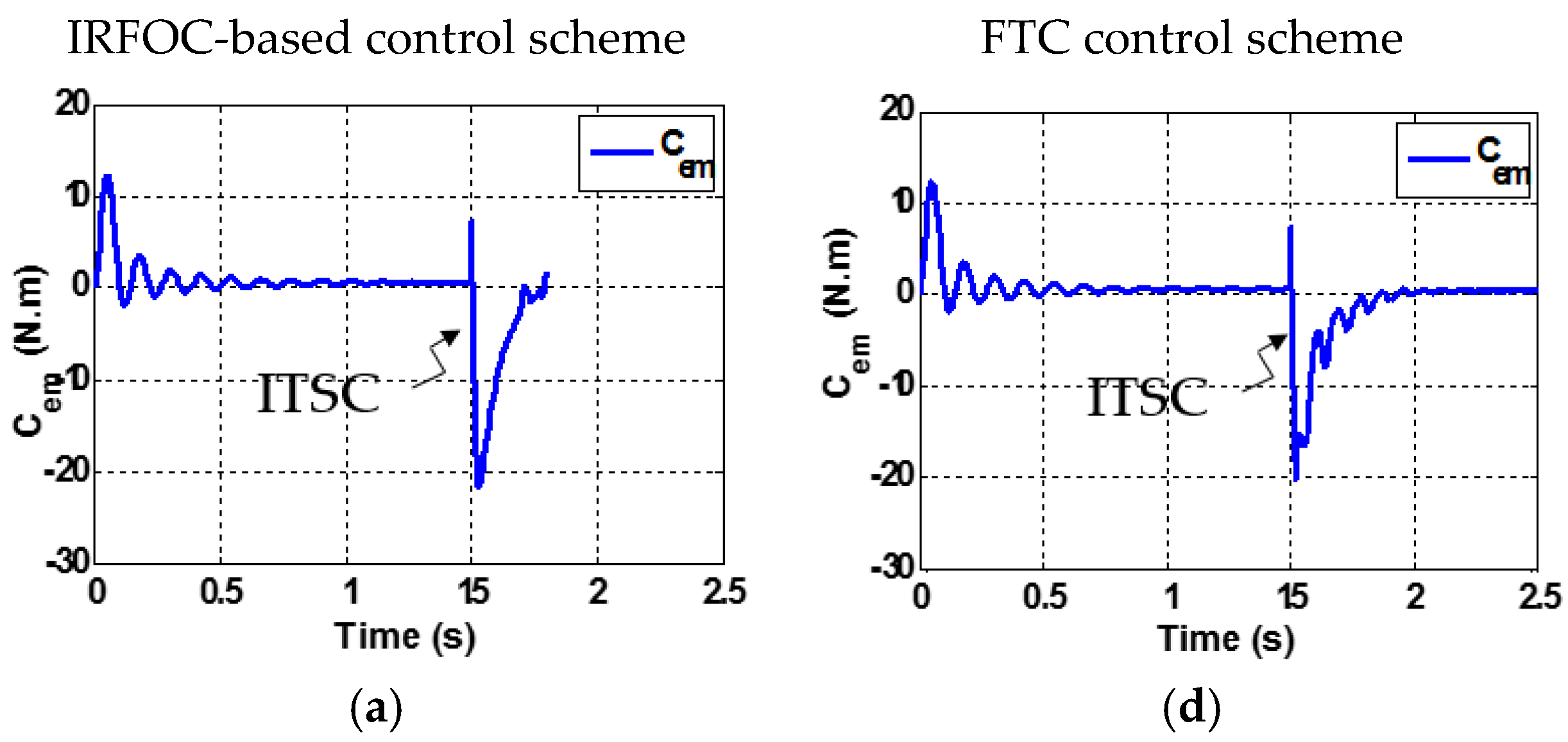
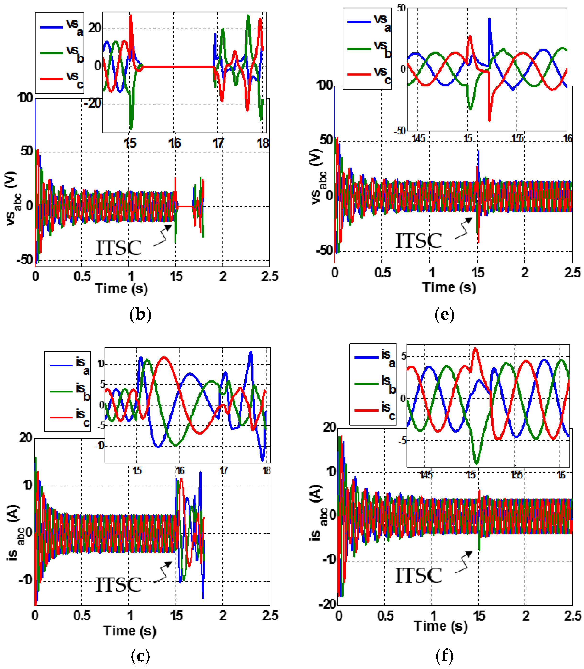
The goal of this section is to investigate the impact of severe ITSC faults (when almost the whole phase is short-circuited) on the subsystems. Thus, a comparison between the signal variations of the first developed control scheme (IRFOC-based control method) and the FTC one is presented under severe faulty conditions. Figure 9 and Figure 10 present both the components of the wind turbine and the grid when an ITSC of 80% of (s₁-phase) is introduced at t = 1.5 s. Figure 9a,d present the variation of the electromagnetic torque C_em. Figure 9b,e present the variation of three-phase stator voltages v^s_abc. Figure 9c,f present the variation of three-phase IG stator currents i^s_abc. Figure 10a,d present the variation of the stator-side converter current i_ch. Figure 10b,e present the variation of P^g the supplied power to the grid. Figure 10c,f present the variation of three-phase grid currents i^r_abc. The results prove that the proposed FTC technique is efficient enough to handle ITSC fault even the most severe ones. It ensures the continuous and reliable operation mode of the system. The control scheme detects the fault presence quickly. The fault phase is isolated. Then the developed scheme compensates the fault impact and restore the equilibrium to the system power phases.

Simulations also show that when the severity of the ITSC fault exceeds a certain level (50% of one phase is short-circuited), the imbalance of IG three-phase currents and voltages becomes so important that it blocks the control scheme and stop the service. Furthermore, the current circulating in the affected phase increases significantly to be destructive to the machine. If the system continues operating under these conditions, the stator-side converter will also be damaged due to the strong current circulating in its legs. Thus, a reliable protection scheme is highly required to isolate the faulty semiconductors and diodes.

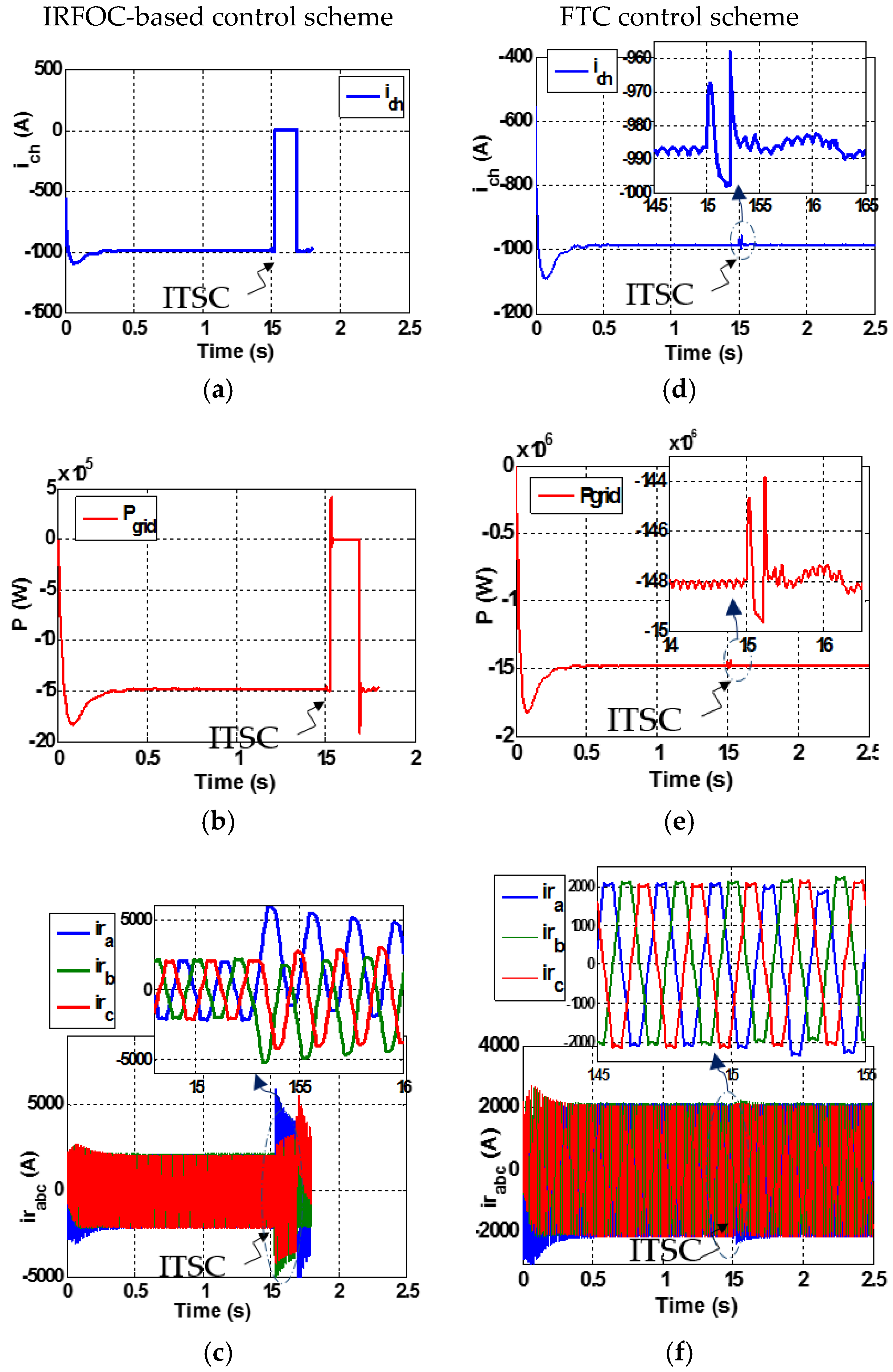
In order to test the robustness of the SMO-based FTC method against both parameter change and wind speed variations, additional simulation tests were run. Thus, a steady wind speed was applied to the turbine (V = 7 m/s), then at t = 1.2 s, the wind speed jumps to reach V = 13 m/s. Furthermore, at t = 1.8 s, an increase of 35% was considered in both the stator and rotor resistance values. Considering the same control parameter values and grid voltage conditions as those set in the previous section, the obtained simulation results test are compared with those got in the previous section, and illustrated in Figure 11. Note that, in spite of the parameter variations and the sudden change in wind speed, SMO are able to estimate the stator currents quickly permitting then a successful achievement of the control targets. This further proves the effectiveness and robustness of the proposed FTC approach in controlling the wind turbine driven IG thanks to the robustness of SMO.

Since this paper deals with ITSC fault, it is important to examine the time variant of the wind turbine system under reactance variations of the stator and rotor phases. Furthermore, to be close to real situations in wind farms, the developed FTC approach is studied under ITSC fault conditions when the wind speed increases suddenly. Thus, Figure 12 and Figure 13 present the simulation result of the developed FTC-Performance of the wind turbine system driven IG with ITSC fault of 30% of s₁-phase under 50% increase in both stator and rotor resistance values at t = 1.5 s and then under a sudden wind speed variation at t = 2.6 s. Figure 12 presents the variation along time of the wind speed V and the mechanical speed ω_mec and its reference ω_mec*. Figure 13 presents the variation along time of the three-phase stator SMO reconstructed currents ${\widehat{i}}_{abc}^s$ and the stator voltages v^s_abc. These results illustrate the robustness of the developed FTC scheme.

6. Conclusions

In this paper, it was shown that inter-turn short-circuit faults engender fluctuations in the stator currents of the generator of a wind turbine. Consequently, the stability of the power supplied to the grid is disturbed which highlights the requirement of an efficient fault detection and isolation scheme and an active fault tolerant control technique to minimize the risk of damage to the generator and stator-side converter. Hence, robust sliding mode observers are developed. The system switches to the proposed SMO-based fault tolerant control scheme once the FDI technique detects a fault. The developed method was able to pinpoint inter-turn short-circuit faults quickly and precisely. It also permits one to isolate the faulty phase, which significantly prevents the propagation of the fault.

When an ITSC fault appears on the generator, the wind turbine system is disconnected from the electrical grid. As proposed in this study, with such a fault tolerant control topology, the wind turbine system can continue operating under nominal conditions with acceptable performance, and consequently, economic benefits can be achieved. Moreover, the fault detection principle detailed in this paper can be used for many faults affecting wind turbine systems.