Dynamic Modeling and Simulation of Deep Geothermal Electric Submersible Pumping Systems


Munich School of Engineering, Research Group “Control of Renewable Energy Systems”, Technical University of Munich, Lichtenbergstraße 4a, 85748 Garching, Germany
*
Author to whom correspondence should be addressed.
Energies 2017, 10(10), 1659; https://doi.org/10.3390/en10101659
Submission received: 21 September 2017
/
Revised: 10 October 2017
/
Accepted: 13 October 2017
/
Published: 21 October 2017
(This article belongs to the Special Issue Low Enthalpy Geothermal Energy)
Abstract
:Deep geothermal energy systems employ electric submersible pumps (ESPs) in order to lift geothermal fluid from the production well to the surface. However, rough downhole conditions and high flow rates impose heavy strain on the components, leading to frequent failures of the pump system. As downhole sensor data is limited and often unrealible, a detailed and dynamical model system will serve as basis for deeper understanding and analysis of the overall system behavior. Furthermore, it allows to design model-based condition monitoring and fault detection systems, and to improve controls leading to a more robust and efficient operation. In this paper, a detailed state-space model of the complete ESP system is derived, covering the electrical, mechanical and hydraulic subsystems. Based on the derived model, the start-up phase of an exemplary yet realistic ESP system in the Megawatt range—located at a setting depth of 950 and producing geothermal fluid of 140 temperature at a rate of 0.145 —is simulated in MATLAB/Simulink. The simulation results show that the system reaches a stable operating point with realistic values. Furthermore, the effect of self-excitation between the filter capacitor and the motor inductor can clearly be observed. A full set of parameters is provided, allowing for direct model implementation and reproduction of the presented results.
1. Introduction
Geothermal energy systems have major advantages compared to other sustainable energy systems: (i) they provide base load power since they are not depending on variable environmental conditions such as wind or sunlight and (ii) they are flexible in their usage as both heat and electrical power may be produced. In so-called low enthalpy regions with reservoir temperatures below 200 [1], p. 32—e.g., the Bavarian Molasse Basin in southern Germany or the Paris Basin in France—electric energy production is made possible by Organic Rankine Cycle (OCR) or Kalina technology. However, in order to efficiently and economically produce electric power with state-of-the-art technology, a geothermal fluid temperature of at least 120 is indispensible [1], p. 43. With an average temperature increase of 3 per 100 depths [1], p. 8, the drilling depths in low enthalpy regions may reach several hundreds to thousands of meters in order to meet the temperature requirements. It is these areas, where deep geothermal systems are typically deployed.
In order to lift the geothermal fluid from the reservoir to the surface, electric submersible pumps (ESP) are employed. Since the ESP technology was predominantly adopted from the oil industry, the systems were not originally designed to withstand the harsh downhole conditions and high volume flow rates required in geothermal power applications [2]. Typical problems involve corrosion, accumulation of carbonate structures (scalings) or insulation failure in the electrical system [3,4,5]. Although ESP manufacturers increased research activity and developed improved designs with higher power and temperature ratings in recent years [3,6], average lifetimes of only a few month—referring to current installations in Germany—remain the bottleneck of the technology [7], p. 62, [8], p. 681.
Reducing the risk of sudden system failure has thus become an important task for operators since unscheduled maintenance and repair services are generally costly and hence to be avoided. Examples of faults in geothermal ESP applications are [8], p. 672:
- Loose cable connections on the motor side (e.g., due to vibrations), leading to an increased electric resistance (possibly differing per phase) and lowering the motor output power.
- Motor insulation faults, resulting in currents among the windings or between the windings and ground.
- Solid parts (scalings) entering the pump, reducing the flow rate and causing fluctuations in the pump pressure and load torque.
- Bearing wear, resulting in higher mechanical friction and overheating of components.
- Shaft fracture, due to abrupt changes in the mechanical load.
One possible solution are condition monitoring systems which may help operators to identify imminent faults at an early stage and consequently perform a scheduled maintenance service in order to prevent catastrophic breakdowns or critical failure. These systems, however, depend on detailed knowledge of the system, obtained through measurements in the downhole and surface equipment, respectively. As downhole sensor data is typically transmitted analogously via modulation onto the supply voltage [9], the signals are highly distorted and hence unsuited for the reliable detection of faults. Other components might simply not be accessible by sensors, impeding further insight into the respective components. This inherent lack of insight into the system state motivates for model-based techniques. In addition, a system model allows for further system analysis, on- and offline simulations and controller design, which makes it a valuable tool for the overall improvement of the ESP system performance and lifetime.
Publications dealing with the modeling and simulation of ESP systems are rarely found. Furthermore, most results are related to oil field applications and provide a limited scope on single subsystems of the ESP only. For instance, Lima et al. describe and simulate an oil field ESP in [10], accounting for the special motor geometry, the mechanical coupling between motor and load and the power transmission through the cable. Although the electrical and mechanical components are described in detail and model sketches are presented, no equations are provided, nor is the hydraulic subsystem treated. Thorsen and Dalva also provide an electrical and mechanical model of an ESP in [11], putting special emphasis on the mechanical resonance observed in the load torque, due to elastic coupling between the individual pump stages. The hydraulic part is neglected, however. Substantial research was also conducted by Liang et al., who analyzed ESP systems for subsea oil applications focussing on load filter design methods and evaluation [12,13] and power transmission via downhole cables [14]. Simulation and experimental results from field studies are provided, yet the exact models underlying those results are not presented. On the contrary, Kallesøe derived a general state-space model of an induction motor coupled with a multistage centrifugal pump [15]. The hydraulic part of the pump was derived by means of 1D streamline theory from fluid dynamics. In the derived model, the transient part of the pressure (head) created by the pump and subsequently the flow dynamics resulting from it are omitted, though. In fact, it is worth mentioning that the transient model of the pump pressure is hardly found in literature with two exceptions, namely [16,17], which solely focus on the hydraulic modeling. A simplified state-space model of a centrifugal pump system is proposed by Janevska in [18], taking into account the reservoir. The electrical system components, however, are not included.
Considering the above findings, to the best knowledge of the authors a complete model of a geothermal ESP system has not been published yet. It is, therefore, the aim of this work to provide a ready-to-use state-space model of a deep geothermal ESP system that allows for a better understanding of the overall system and serves as a foundation for the development of model-based (online) condition monitoring strategies, state observers (as sensor surrogates or for redundancy) and sophisticated control algorithms. Inputs to the model are high quality surface measurements—as opposed to the often unreliable and noisy downhole measurements—of the voltages, currents and flow rate, respectively, allowing for on- and offline simulations of the system and testing of the developed algorithms. A system theoretical modeling approach covering the electrical, mechanical and hydraulic subsystem is chosen, which is based on deriving the state-space descriptions from physical relations of the various system states, expressed as a set of nonlinearly coupled first-order differential equations.
2. State-Space Model of Deep Geothermal ESP Systems
In this section, a nonlinear state-space model is derived, laying the foundation for implementations and further system analysis. As the main objective of this paper is to provide a modular system model that can easily be implemented and extended in simulation software, each component is modeled separately, allowing for convenient exchange of single components. Although the aim is to map the physical system in as much detail as possible, generally a trade-off between model complexity and accuracy must be found. It may therefore be necessary to impose simplifying assumptions in order to obtain a state-space description.
An overview of the whole ESP system, its three subsystems and their components is given in Figure 1. The basic components of the ESP system with variable speed drive (VSD) are (see e.g., [3,10,13]):
- Voltage-source inverter (VSI) (producing variable frequency and amplitude output voltages),
- Sine filter (converting the pulsed VSI output voltages into almost sinusoidal voltages),
- Cable (transmitting the electrical power to the downhole motor),
- Motor (driving the pump by converting electrical into mechanical power),
- Protector (Seal) (serving as axial bearing and oil reservoir placed between motor and pump),
- Shaft (transmitting the mechanical power from the motor to the pump),
- Pump (generating pressure by converting mechanical into hydraulic power), and
- Pipe system and geothermal reservoir (representing the hydraulic load).
In the derived model, the Protector is considered to be a part (extension) of the shaft and is therefore included in the shaft model, without further elaboration on axial forces acting on the motor and pump, respectively. Based on the considered component selection, the nonlinear state-space models of the electrical, mechanical and hydraulic subsystems are derived in the following.
2.1. Electrical Subsystem
The electrical subsystem covers the inverter, sine filter, cable and motor. Based on three-phase equivalent circuits, a two-phase description is derived for each component, yielding expressions for the inputs and output currents and (phase) voltages, respectively. The phase voltages are stated with respect to the reference potential measured at the motor star point , which is further specified in the motor section.
2.1.1. Inverter
The power converter links the grid with the electrical drive system and is typically given in back-to-back configuration, with a grid-side voltage source inverter (VSI), a common DC-link and a motor-side VSI. Instead of the grid-side VSI (active front end), which allows bidirectional power flow, a diode bridge may alternatively be used as a rectifier, if the electric power is supposed to flow from the grid to the machine only. The model derived in this paper assumes a constantly charged DC-link capacitance (see Assumption 2) and hence restrains to the motor side. The motor-side VSI serves as a voltage and power source for the electrical machine of the pump, generating sinusoidal voltages of variable frequency and amplitude according to a specified reference voltage. In this paper a 5-level active neutral point clamped (ANPC-5L) inverter as described in [19] is employed, which is well-suited for medium voltage drive applications.
The schematic of a single phase of the inverter is depicted in Figure 2. Each phase a, b or c of the inverter consists of three cascaded cells with a total of eight power switches per phase. The input is accessed via the terminals and while the output voltages are taken from the terminals , respectively. Moreover, the phase current flows out of the inverter. The power switches of phase k—typically given as insulated-gate bipolar transistors (IGBT)—are controlled by the three switching signals (the respective inverse signals are denoted by , and ). Cell 1 is controlled by switching signal , with switches 1 and 3 (counted from top to bottom) and switches 2 and 4 controlled in pairs. Cell 2 consists of two complementary switches controlled by , as does cell 3 which in turn is controlled by .
Assumption 1 (Ideal switches).
The inverter IGBTs are assumed ideal switches with switching levels ’1’ (closed) and ’0’ (open), i.e.,
- no current may flow if the switch is open,
- bidirectional current may flow without voltage drop, if the switch is closed and
- the switching takes place instantaneously (no switching delay).
The input DC-link capacitances are shared between the three phases, whereas the capacitance is assigned to each phase individually [19]. While is charged by the grid-side rectifier or VSI, is charged by exploiting redundant switching-states and thus controlling the current flowing into or out of the capacitance (i.e., “voltage balancing”). As sophisticated inverter control algorithms are beyond the scope of this paper, the following assumption is made.
Assumption 2 (VSI capacitance).
The inverter capacitances and are charged to defined voltage levels and and are assumed constant for all times.
The switching combinations and resulting output voltages of phase k are listed in Table 1. The corresponding current paths are indicated in Figure 2 by the colored lines, which comply with the background colors of the table rows. Although three switches allow for eight different switching combinations, the line-to-neutral voltage (in ) measured between the output terminal and the neutral point can attain five distinct voltage levels, i.e., . This aforementioned redundancy can be used to charge the phase capacitance . However, the exact switching combinations leading to the different voltage levels are irrelevant for the model presented in this paper and therefore the overall switching signal is used to summarize and describe the overall switching-state and its respective output voltage level for phase k.
Hence, the overall three-phase switching-state vector can be introduced such that the line-to-neutral voltages may be written as:
The line-to-line voltages measured between the inverter outputs , and (see Figure 2) can in turn be expressed in terms of the line-to-neutral voltages as:
yielding nine different output voltage levels, i.e., . Moreover, the line-to-line voltages may be expressed as , where are the phase voltages measured between the output terminals of the inverter and the motor star point . Since the matrix is not invertible, the equation cannot be solved for [20], Chapter 14. However, making use of the general voltage constraint (with possibly non-zero offset voltage , if the phase voltages are not balanced), the phase voltages can be stated as:
As a two-phase representation is preferred here, the reduced amplitude-correct Clarke transformation and its (pseudo) inverse are introduced as (see e.g., [20], Chapter 14)
Employing the transformation matrices defined in (4), vectors may be transformed by and matrices by , respectively. Finally, the phase voltages and currents at the inverter output can be expressed in -coordinates as
In the -reference frame, the feasible phase voltages can be visualized by the voltage hexagon as shown in Figure 3. The respective switching combinations leading to each node are given in the circles attached to them (e.g., ).
In general, the objective of the VSI is to reproduce a given voltage reference vector at its output terminals. In order to achieve this goal, the desired voltage is sampled with switching frequency (in ) and translated into the time domain by modulation of the switching signal, using e.g., sinusoidal pulse width modulation (SPWM) or space vector modulation (SVM). As a result, the sliding time integral (moving average) of the output voltages over a defined sampling period (in ) matches the reference voltage sample, i.e.,:
A space vector modulation algorithm for 5-level inverters has been implemented based on [21].
2.1.2. Filter
The VSI generates voltage pulses with steep slopes (high ) which (i) increase harmonic losses and (ii) put high stress on the insulation due to parasitic cable and motor capacitances [22]. Moreover, the high inductance of the motor windings causes (iii) wave reflection at the machine terminals with a reflection factor of almost one [23], requiring a voltage derating since the reflected voltage may reach twice the original amplitude [23]. An effective way of avoiding the mentioned effects is to employ an LC ouput filter (lowpass filter) that smoothes the output voltages and thus reduces steep voltage slopes. The output filter is located between the VSI output and the downhole cable (see Figure 1).
The equivalent circuit of a non-ideal LC-filter is shown in Figure 4. The filter resistance matrix is given by (in ), the filter inductance matrix by (in ) and the filter capacitance matrix by (in ).
The star point of the wye-connected capacitances is not grounded and hence at floating potential, i.e., at voltage with respect to the motor star point. Moreover, the input voltages are denoted by (in ), the input currents by (in ), the output voltages by (in ) and the output currents by (in ).
Using Kirchhoff’s current and voltage laws on nodes ⓪ to ③ and meshes ![Energies 10 01659 i001]() to
to ![Energies 10 01659 i002]() , respectively, yields
where is the voltage between star point of the capacitor bank and the star point of the motor. Since , the term ⊛ in (8) vanishes if the reduced Clarke transformation is applied, thus yielding the reduced state-space representation in the -reference:
with state vector , input vector , system matrix and input matrix . Note, that the input voltage vector is equal to the VSI output vector and the output current vector depends on the load connected to the filter output.
, respectively, yields
where is the voltage between star point of the capacitor bank and the star point of the motor. Since , the term ⊛ in (8) vanishes if the reduced Clarke transformation is applied, thus yielding the reduced state-space representation in the -reference:
with state vector , input vector , system matrix and input matrix . Note, that the input voltage vector is equal to the VSI output vector and the output current vector depends on the load connected to the filter output.
 to
to  , respectively, yields
2.1.3. Cable
The power cable connects the filter output with the electrical machine and runs through the space between wellbore and production tubing. As it extends over the whole distance, from the filter output to the motor, the cable length (in ) becomes a crucial parameter regarding the electrical properties of the cable such as resistance, inductance and capacitance, also known as line parameters and typically stated per-unit-length (p.u.l.).
The standard models for power transmission lines are derived by invoking a distributed parameters approach, which allows the modelling of an infinitesimally short fraction of the cable as a combination of p.u.l. series impedance and shunt admittance. This approach leads to a set of partial differential equations, called Telegrapher’s equations (see e.g., [24]), whose steady-state solution are time and space dependent wave functions for voltages and currents, respectively. As the distributed parameters approach leads to an infinitely large number of states, a discretization of the model using lumped parameters and a finite set of cable segments is performed. For sufficiently short segments the space dependency can be neglected and the segments can be approximated by equivalent - or -circuits. A segment is classified short if the wavelength (in ) of the voltage and current waveforms is at least 60 times larger than the segment length, i.e., holds [25], p. 426. Given the vacuum speed of light (in ), the relative permeability of the cable insulation and the frequency of the driving signals f, the condition can be refined to (see [25], p. 410):
It can be concluded from (10) that, even without a sine filter and switching harmonics of up to 2 , the maximum cable length of covers most geothermal power applications and hence a single sequence of - and -segments is sufficient for modeling the cable.
Nevertheless, in the presented model two segments are used: A -segment of length is used on the filter side, as the input voltage is a state variable due to the output capacitance of the filter, and a -segment of length is used on the load side of the cable, due to the input inductance of the electric machine. Considering the electric and magnetic coupling between the conductors, the circuit elements are derived from the p.u.l. line parameters.
Assumption 3 (Cable shunt conductance).
It is assumed that the shunt conductance of the power cable is negligible [25], p. 430.
The remaining line parameters are given by (in ), (in ) and (in ), denoting the p.u.l. cable resistance, inductance and capacitance matrices.
Magnetic coupling is described by the p.u.l. inductance matrix which is defined as the constant ratio of conductor flux linkages and currents (if magnetic saturation is neglected), divided by the segment length , i.e.,:
Moreover, electric coupling is represented by capacitances between the lines and ground, respectively. It can be shown (see Appendix B and [26]) that the capacitances used in the equivalent circuits, i.e., the line-to-ground capacitances and line-to-line capacitances (in ) for , are related to the line capacitances used in the phase description by:
The equivalent circuit of the -segment is shown in Figure 5, with input voltages (in ), input currents (in ), output voltages (in ), output currents (in ) and voltages across the capacitances (in ). Moreover, the -model parameters are given by (in ), (in ) and (in ). Note that, for inductances and resistances, half of the respective values were considered on the input and the other half on the output of the -segment (that is why appears in the expressions above).
As in the previous section, the state-space description can be derived using circuit analysis. For the -model, evaluating meshes ![Energies 10 01659 i001]() to
to ![Energies 10 01659 i002]() , meshes
, meshes ![Energies 10 01659 i003]() to
to ![Energies 10 01659 i004]() and nodes
and nodes ![Energies 10 01659 i005]() to
to ![Energies 10 01659 i006]() yields
where denotes the voltage between motor star point and ground. Applying the reduced Clarke transformation as in (4) eliminates the term ⊛, i.e., , such that the state-space description of the -segment in the -reference frame can be stated as
with state vector , input vector , system matrix and input matrix . For the -segment, the input voltage is equal to the filter output and the output voltage is determined by the input voltage of the -segment.
yields
where denotes the voltage between motor star point and ground. Applying the reduced Clarke transformation as in (4) eliminates the term ⊛, i.e., , such that the state-space description of the -segment in the -reference frame can be stated as
with state vector , input vector , system matrix and input matrix . For the -segment, the input voltage is equal to the filter output and the output voltage is determined by the input voltage of the -segment.
to , meshes  to
to  and nodes
  to
to  yields
Likewise, the -model state-space form can be derived. The equivalent circuit of the -segment is shown in Figure 6, with input voltages (in ), input currents (in ), output voltages (in ), output currents (in ) and currents through the inductances (in ). The -model parameters are given by (in ), and (in ) and (in ).
The system description is obtained by evaluating meshes ![Energies 10 01659 i007]() to
to ![Energies 10 01659 i008]() , nodes
, nodes ![Energies 10 01659 i009]() to
to ![Energies 10 01659 i010]() and
and ![Energies 10 01659 i011]() to
to ![Energies 10 01659 i012]() , i.e.,
, i.e.,
 to
to  , nodes
  to
to  and
and  to
to  , i.e.,
Applying the reduced Clarke transformation, the disturbance ⊛ is eliminated, i.e., , and the state-space description for the -segment is given by
with state vector , input vector , system matrix and input matrix . For the -segment the input currents are determined by the output currents of the -segment, whereas the output currents depend on the load connected at the cable end.
2.1.4. Electrical Machine
The electrical machine drives the pump. Both are mechanically linked via a shaft. In order to achieve higher power output, two separate motors may be connected in series, which is known as tandem configuration [27]. Typically, squirrel-cage induction motors are used, since they are well-known, cheap and robust. However, as high currents are flowing through the rotor bars and resistive losses (heat) are proportional to the current squared, induction machines tend to heat up quickly. Moreover, the only feasible way to cool the machine is the use of hot geothermal fluid to conduct away the heat. Therefore, the ampere rating has to be kept at a minimum level, which requires a higher voltage rating of the machine in order to guarantee the desired mechanical output power.
Due to space limitations inside the borehole, the motor dimensions have to be adapted, resulting in a long axial expansion and a small diameter. While the stator windings typically expand over the whole length of the motor, the rotor on the other hand is segmented, with each segment isolated from each other and equipped with its own bearings [28]. Moreover, the space between rotor and stator is filled with oil as to (i) prevent water from entering the machine, to (ii) accommodate the high ambient pressure and to (iii) improve heat transfer from the rotor to the motor surface in radial direction [28].
Assumption 4 (Motor modeling).
It is assumed that
- the motor is star-connected, i.e. the secondary ends of the phase windings are interconnected at the motor star point ,
- the multi-rotor configuration can be considered a single rotor with combined electromagnetic properties, i.e., no torsional effects among individual rotors are considered, and
- iron losses can be neglected.
The resulting three-phase equivalent circuit is shown in Figure 7, with stator voltages (in ), stator currents (in ) and stator flux linkages (in ), rotor currents (in ), rotor flux linkages (in ) and rotor angular velocity (in ), respectively. The rotor variables are related to the stator [29] and expressed in stator fixed -coordinates.
The stator windings (phases) are modeled by the stator resistances (in ) and the stator inductance (in ), where can be separated into the stator stray inductance (in ) and the main inductance (in ), i.e., [29]. The main inductance causes magnetic coupling between the rotor and stator phases which can be expressed in terms of the stator and rotor flux linkages.
Assumption 5 (Magnetic linearity).
It is assumed that the effect of magnetic saturation can be neglected and hence the stator and rotor flux linkages are affine functions of the stator and rotor currents, respectively, i.e.,
In the fault-free case, the phase resistances are typically identical, i.e., holds. However, in case of windage faults this assumption may not hold true anymore and therefore the general description is used in the presented model. For the sake of consistency, the same applies for the rotor resistances.
The stator voltages, measured between the input terminals and the motor star point , are given by:
Applying the Clarke transformation (4) yields the corresponding representation in the -reference frame:
On the rotor side, the conducting bars of the rotor cage are likewise modeled as a three-phase system, with rotor resistance (in ) and rotor inductance , composed of the rotor stray inductance (in ) and the main inductance , i.e., [29]. Moreover, the rotor magnetic field induces a voltage in the rotor cage depending on the flux linkage and the electrical (synchronous) speed , where (in ) is the mechanical speed and is the number of pole pairs. Evaluating meshes ![Energies 10 01659 i016]() ,
, ![Energies 10 01659 i017]() and
and ![Energies 10 01659 i018]() yields the following dependency:
which, transformed to -coordinates, becomes:
where and:
yields the following dependency:
which, transformed to -coordinates, becomes:
where and:
 ,
,  and
and  yields the following dependency:
Solving (22) for allows to eliminate the rotor currents from (19) and (21) and, hence, the overall nonlinear state-space electrical system can be derived as follows:
where denotes the inductive leakage factor, is the state vector, is the input vector, is the non-linear system function and is the input function. Note that the rotational speed describes an additional system state which results from the torque balance on the machine shaft, i.e.,:
where (in ) is the overall moment of inertia, (in ) is the motor torque and (in ) is the sum of load torques acting against the motor torque. In anticipation of the mechanical subsystem, the electro-magnetic torque (in ) produced by the motor can be described in terms of electrical system states, i.e., (see e.g., [20], Chapter 14):
The load torque and inertia, however, are determined by the hydraulic and mechanical subsystems derived in Section 2.2 and Section 2.3. Therefore, the rotational speed dynamics will be further elucidated in the following sections.
2.2. Hydraulic Subsystem
The hydraulic subsystem comprises the pump and the piping system. The former serves as a hydraulic source, while at the same time being a mechanical load. The latter in turn is the hydraulic load. The produced volume flow results from the net head, i.e., the difference between hydraulic source and load.
2.2.1. Pump
The pump is used to lift the geothermal fluid from the deep well to the surface and thus forces it to overcome a height difference. In order to produce the required volume flow rates—despite the strict space limitations in geothermal power applications—multi-stage centrifugal pumps are employed. Each stage of the pump consists of a moving part, the impeller, and a fixed part, the diffuser. In the impeller the fluid is accelerated, whereas the diffuser converts the kinetic energy into static pressure, and thus performs hydraulic work.
Figure 8a shows the 2D cross-section of a centrifugal pump impeller, which defines the control volume as a function of cross-section area (in ) and uniform impeller height (in ). The fluid enters the impeller through the inlet area at radius (in ) and leaves the impeller through the outlet area at radius (in ). Due to its axisymmetric design, the shape of the blades depends on the radius r only and is described by its angle (in ), with inlet angle and outlet angle , respectively. The movement of the fluid particles is described by the velocity triangle (see Figure 8b) at every point in , where and v (in ) are tangential, relative and absolute speed, respectively. Moreover, the impeller rotates with angular velocity , imposed by the motor through the shaft. The total volume flowing through the pump stage is described by the volume flow (in ) and is the result of the produced head (in ), describing the height of the water column potentially produced in the pump stage. For an incompressible fluid (see Assumption 6), the density (in ) is constant and thus head becomes proportional to static pressure. Furthermore, the impeller creates a load torque (in ) acting on the shaft. Both, load torque and head, depend on the rotational speed and the volume flow. The respective hydromechanical model of the pump is derived based on 1D average streamline theory of fluid dynamics in Appendix A. It is subject to the following assumptions:
Assumption 6 (Incompressible flow).
The geothermal fluid is assumed to be incompressible, i.e., (constant).
Assumption 7 (Average streamline).
The velocity distribution of the fluid particles within is assumed to be uniform, i.e., the velocity triangle depends only on the radius r, but not on the angle ϕ.
As derived in Appendix A.1, the load torque created by a single stage of the impeller is described by:
with geometry dependent constants (in ), (in ), (in ), (in ) as defined in (A8) and (in ) accounting for disk friction losses. Note that describes the inertia of the fluid contained in the impeller, whereas describes the impact of flow rate variations on the load torque.
The head created by a single impeller stage is derived in Appendix A.2 and given by:
with constants (in ), (in ), (in ), (in ) and (in ). While is the (head related) fluid inertance, describes the impact of change of the rotational speed on the produced head. The steady-state parameters and depend on the geometry, but also account for hydraulic losses such as hydraulic friction, shock losses and the slip factor [15]. A qualitative H-Q-curve for constant is depicted in Figure 9: At the absence of losses, the pump produces the theoretical head, which is drawn as a bold line. Due to the finite number of impeller vanes and flow deviations from the mean line, the theoretical head is decreased by a constant factor (slip factor), indicated by the hatched blue area. Incidence (hatched yellow area) and skin friction (hatched green area) losses depend quadratically on the flow, resulting in the parabolic shape of the curve. At the best efficiency point (BEP), the pump operates at designed conditions and the losses are minimal. Further details on the loss mechanisms can be found in Appendix A.2.
Deep geothermal ESP systems are deployed at great depths, such that the required head cannot be produced by a single pump stage anymore. For this reason, multi-stage pumps are used, with each stage adding to the total head, as well as increasing the overall load torque.
Assumption 8 (Multi-stage characteristics).
Each impeller stage is assumed to contribute equally to the total head and load torque, respectively.
As a consequence of Assumption 8, the series connection of N pump stages can be accounted for by multiplication of the single stage load torque and head with factor N. Ideally, the volume flow through the impeller stages should be the same as the flow leaving the pump discharge. However, due to leakage in the seals, wearing rings, bushings and axial thrust balancing devices a small portion of the flow is lost [30], Section 3.6.2. Leakage flow occurs particularly at partload as the high pressure fluid cannot exit the pump through the outlet and hence flows back through narrow passages to the lower pressure regions. For the sake of simplicity the following assumption shall hold.
Assumption 9 (Leakage flow).
It is assumed that the leakage flow is much smaller than the main flow and thus negligible, i.e., holds true.
2.2.2. Pipe System and Geothermal Reservoir
The hydraulic system between pump intake and wellhead defines the hydraulic load of the model. It is depicted in Figure 10 and comprises the production pipe, pressures at both pipe ends and the (dynamical) water level.
Assumption 10.
The production pipe radius (in ) is assumed constant, such that the (steady-state) flow velocity can be considered uniform along the production path.
In view of Assumption 10, the system head (hydraulic load) can be described by the dynamic (transient) Bernoulli equation for incompressible, inviscid flow along a streamline as [31], Chapter 6.6:
with system flow (in , equal to the pump flow) and an additional loss term to account for the frictional losses in the piping system. The constant (in ) denotes the inertance of the fluid in the piping system, whereas (in ) is the combined hydraulic friction coefficient. Both coefficients, and , linearly depend on the water level and thus dynamically change during the system start-up. The friction coefficient is derived using the Darcy-Weisbach Equation (see e.g., [30], Section 1.5.1), i.e.,:
where (dimensionless) denotes the Darcy friction factor depending on the Reynold’s number of the pipe system. The inertance on the other hand is given by:
and follows from the integral along the streamline of the water (see e.g., [31], Chapter 6.6). The term:
denotes the part of the system head (in ) which consists of the (limited) water column weighing on the pump and the scaled pressure gradient between wellhead pressure and reservoir pressure (in ). While the wellhead pressure is typically kept at a constant value once it reaches a required value, the reservoir pressure changes throughout the operation of the system, resulting in a lower idle water level (drawdown). The drawdown is characterized by the productivity index (in ) of the geothermal reservoir and the idle pressure (in ) and changes with the volume flow. According to [8], Section 14.1.2 the reservoir pressure can be stated as:
Moreover, the dynamic water level can be described by the following equation
where:
allows for conditional activation or deactivation of the integration in (33). The wellhead pressure is built-up only if the water column reaches the wellhead and is saturated by a defined (and constant) value (in ), according to the employed pressure valve. It can be described by:
with decision function:
The equilibrium condition of the hydraulic system can be obtained by enforcing , which is obtained by inserting (27) and (28) into the balance condition, i.e.,
where (in ) is the overall inertance of the fluid in the system and (in ) the static head. Note that the amount of water in the pipe is typically much higher compared to the water in the pump and thus the overall intertance can be approximated by . The above equation fully describes the dynamics of the hydraulic system. However, as it depends on the derivative of the rotational speed, the mechanical system has to be taken into account in order to resolve this dependency.
2.3. Mechanical Subsystem
The mechanical subsystem links the electrical with the hydraulic subsystem as it transfers the motor torque via the shaft to the pump, which in turn imposes a load torque on the shaft. According to Newton’s second law, the shaft is accelerated in proportion to the net torque applied. As proposed by [10,11], the shaft is modeled as an elastic spring-damper-system due to its high length-to-diameter ratio. For the sake of simplicity lumped parameters are used to describe the two-mass system [20], Chapter 11.
2.3.1. Shaft (Spring-Damper-System)
A rotational spring-damper-system is depicted in Figure 11. Both, motor and pump, are modeled as rotating masses with motor and impeller moments of inertia and (in ), angular displacement angles and (in ), angular velocities and and viscous friction coefficients and (in ), respectively. The shaft is modeled as a massless link between motor and pump with torsion constant (in ) and damping coefficient (in ).
Applying Newton’s second law and considering torsion and damping moments, the mechanical system is described by the following equations
Inserting the electromagnetic torque of the motor (25) in the motor-side mechanical system (38) and solving for yields the motor-side mechanical system:
Similarly, the impeller load torque (26) can be inserted in the pump-side mechanical system (39) yielding the hydromechanical coupling
Note that both, the derivatives of flow and angular velocity appear in the this equation, which does not comply with the standard form of state-space representations (i.e., ).
Assumption 11 (Flow dynamics).
It is assumed that the overall hydraulic system is considerably slower than the mechanical system (as proposed in [15]), i.e.,
holds at all times.
As a consequence of Assumption 11 the term in (41) is negligible and the pump side mechanical system can be written as:
where (in ) is the overall moment of inertia and (in ) the overall viscous friction coefficient of the pump.
2.3.2. Decoupling of the Hydraulic and Mechanical System Dynamics
In order to obtain the state-space representation in standard form, the pump-side speed and flow dynamics need to be merged by combining (38), (40) and (43) and solving for , i.e.,
Input of the hydraulic system is the static head .
2.4. Overall System Dynamics
Having derived the submodels of the pump system—i.e., Equations (9), (14), (16), (23), (40), (43) and (44)—the inputs and outputs can be connected and the overall system stated in a single equation as
with state vector , system function , input function and input vector . The colors indicate the subsystem of the respective state variables, i.e., electrical (red), mechanical (orange) and hydraulic (blue) subsystem.
3. Simulation Results and Discussion
The state-space submodels as derived in the preceding sections and summarized in (45) have been implemented in MATLAB and Simulink (R2017a, The MathWorks, Inc., Natick, MA, United States) using the parameters given in Table 2, Table 3 and Table 4. The parameters were either calculated based on estimated geometry and system data—e.g., inverter, filter, cable—or provided by local energy suppliers (As to avoid conflicts with existing nondisclosure agreements, the suppliers’ data has been modified in such a way that the values remain realistic yet do not represent real values)—e.g., hydraulic system, pump, motor, shaft. The simulations have been performed using the ode4 solver with a fixed step time of 100 for the duration of 100 . The displayed data was sampled at the end of each PWM cycle, since at this point the voltage over time integral of the inverter output voltage equals the voltage over time integral of the sampled reference voltage.
3.1. Test Scenario
For the simulation, the system is assumed to be in idle state, initially. The geothermal reservoir lifts the fluid to its idle water level of approximately m below surface level and the ESP system is at standstill with zero voltage applied. In the start-up phase, Regime I (), the reference voltage magnitude and frequency are increased simultaneously (u/f control) at a constant ratio of 96.2 with slopes of 144.3 and 1.5 , respectively. Once the maximum values are reached, the voltage references are kept constant. In Regime II (), the hydraulic system is in transient state; while in Regime III (), the overall system is in steady state.
3.2. Results and Discussion
The simulation results are depicted in Figure 12, Figure 13, Figure 14 and Figure 15; with Figure 12 showing the pump characteristic curves and the respective trajectories of operating points, Figure 13 showing the general system behaviour of the different physical subsystems, Figure 14 showing power related simulation data and Figure 15 showing detailed views of the electrical (see Figure 15a,b) and mechanical (see Figure 15c) simulation results. The pump curves in Figure 12 and Bode diagrams in Figure 16 are used to further illustrate the pump behaviour and validate the hypotheses inferred from the timeseries plots. Whenever necessary, the measured data was filtered by a moving average filter to improve the display of multiple timeseries within one plot. The mean values are plotted as solid lines, whereas the original data is moved to the background with the same color but lower opacity.
3.2.1. Overall System (See Figure 13)
In the first plot (from top to bottom) of Figure 13, the voltage magnitudes measured at the inputs of the different electric system components are plotted, i.e., the filter input (inverter output) voltage , the cable input (filter output) voltage and the machine input (cable output) voltage . As described in Section 2.1.1, the inverter output (filter input) voltage switches between nine discrete voltage levels, varying around the desired reference voltage with large deviations, yet accurate on average per sampling period. Therefore, the filter input voltage can be represented by the sampled and delayed (for one switching period) reference voltage, fed to the inverter. As expected, the filter input voltage magnitude is increased linearly during Regime I and equals in Regimes II and III. The damping resistor of the filter and the resistive part of the power cable lead to voltage drops which can be observed in the slightly smaller magnitudes of the cable and stator voltages, respectively.
The second plot shows the corresponding current magnitudes, with filter input current , cable input current , stator current and rotor current . The first observation is that the cable and stator currents almost perfectly coincide, which leads to the conclusion that the influence of the cable on the dynamic system narrows down to a mere voltage drop, assuming that a filter is employed. This hypothesis is supported by the Bode diagram of the open-loop power cable transfer function , which is given in Figure 16b. The transfer function is deduced from the system Equation (45). From the Bode diagram it can be inferred that no significant changes in magnitude and phase occur in the operating frequency range of 0 to 60 . In fact, even the lowest resonance point located in the frequency range of 30 to 40 is very unlikely to be excited.
Another important observation is that—after a brief initialization period—the filter current becomes smaller than the stator current, which implies that current is circulating between the filter output and the motor. This effect is known in literature as self-excitation [32] and should be taken into account when designing the filter, since higher currents than measured at the inverter output will flow into the filter capacitors. Further analysis of this is effect is conducted in the power section, when looking at the reactive power flow.
The third plot of Figure 13 shows the speed measured at the electrical machine output and the pump input , respectively. Due to the frequency ramp until the machine speeds up during Regime I, reaching a final value slightly below 377 (60 ), which is caused by the slip of the induction machine.
In the fourth plot, the machine torque produced by the motor and the load torque of the pump are shown. It can be observed that the load torque is directly related to the volumetric flow rate (6th plot), which increases during start-up, then is slightly reduced and finally reaches steady-state at . Due to friction and damping in the mechanical system, the motor must provide a higher torque than actually required by the load which can clearly be observed in the plot. Moreover, the motor torque is subject to an apparent ripple which is caused by the current ripples (as a consequence of inverter switching).
The fiths plot shows various pressures and water levels in terms of head, with pump head , water level and draw down . As expected, the pump head is proportional to the speed squared and thus shows a parabolic increase during Regime I. It can be observed that the pump head is slightly reduced after the start-up procedure is completed (Regime II), which might be caused by the high fluid inertance that causes the flow to increase, even though further head is not delivered in terms of increased pump speed. When the flow settles at (Regime III), the pump head reaches its final value and the overall pump system is in steady-state. The corresponding pump flow is shown in the sixths (last) plot.
In addition, Figure 12 shows contour plots of the simulated pump system, with (a) the trajectory of the pump operating points (red line) over the HQ-contour plot of the simulated pump and (b) its respective input power as defined in (47) (PQ-contour plot). The dashed white line in the HQ-curve represents the system curve for zero wellhead pressure, whereas the solid white line assumes full wellhead pressure as defined by . In Figure 12a, the trajectory in the HQ-curve shows that after a short acceleration period, the pump reaches its maximum flow rate at constant speed slightly below 60 . From here, constant speed is maintained and the trajectory starts moving on the respective hyperbola. When the trajectory crosses the dashed white line the height difference between pump and wellhead is overcome. Finally, the trajectory reaches the solid white line, where the desired wellhead pressure is reached. In Figure 12b, the parabolic power input (due to constant and linear increase of ) during the acceleration phase (Regime I) is clearly visible, whereas in Regime II only the pump head is further increased while the pump load torque decreases (see Figure 13). This leads to a reduction of the pump input power until its final value of is reached in Regime III (compare also with first plot in Figure 14).
3.2.2. Power and Efficiency (See Figure 14)
In the following, electrical power terms such as apparent, active and reactive power will be used. For voltage and current vectors and , the averaged (RMS) power terms are defined as
with sampling period , active power P (in ), reactive power Q (in ) and apparent power S (). Moreover the power factor is defined as .
The first plot of Figure 14 (likewise from top to bottom) shows various power terms related to the pump system, i.e., motor electrical input power , motor mechanical output power , pump mechanical input power and pump hydraulic output power (all in ), i.e.,
As power is flowing in the aforementioned order—from the motor input to the pump output—and losses occur in each subsystem a steady decrease in power can be observed. The corresponding efficiencies are shown in the second plot, with denoting the motor efficiency and denoting the pump efficiency, respectively. The motor efficiency reaches values of over 90%, while the pump efficiency is much lower with a maximum value of about 70%. The efficiency of the overall system is given by with a maximum value of approximately 60%, where denotes the active power at the filter input.
Plots 3–5 show the apparent, active and reactive power components, measured at the filter input (subscript ), cable input (subscript ) and machine stator (subscript ), respectively. The apparent power shows similar characteristics as the current magnitudes depicted in Figure 13, with a higher apparent power in motor and cable, compared to the filter. On the contrary, the active power is steadily reduced from filter to motor, as resistive components in the system dissipate power. Looking at the reactive power, it can be observed that the inverter supplies reactive power to the system in the interval . At approximately the reactive power flow ceases, whereas for the inverter consumes reactive power. In order to analyze this effect the Bode diagram for the no-load case (i.e., no current is flowing in the rotor) can be consulted. As mentioned above, the cable can be neglected in the analysis. The Bode diagram is shown in Figure 16a for two different transfer functions, i.e., and . The magnitude plot reveals that the filter current is damped with approximately 70 dB at frequency , which explains that no reactive power is flowing at the filter input for that specific frequency (at the reference frequency equals ). As a consequence, reactive power must circulate between motor and filter. This hypothesis is supported by the resonant frequency of the filter capacitance and the stator inductance . At the same frequency, a phase shift of 180 in the filter current occurs. Since both, stator and filter current, are defined positive in the same direction, the phase shift of the filter currents means that both currents flow simultaneously into the filter capacitor and thus lead to high currents in the capacitor.
In the sixth plot, the corresponding power factors are depicted. As expected, the filter power factor reaches 1 at , since the reactive power flow is zero. Moreover, it can be observed that during start-up (Regime I) an increased amount of reactive power—compared to active power—is required as the electromagnetic components are supplied, while at the same time the load (active part) is not fully built up yet, resulting in a low power factor.
3.2.3. Detailed Views on Electrical and Mechanical Subsystems (See Figure 15)
Figure 15a,b show detailed views of the voltages, currents and flux linkages (for phase ) of the various electrical subsystem components for two different operating points (Regime I in Figure 15b and Regime III in Figure 15a). Both plots show three periods of the sinewave signals, with fundamental frequencies 22.5 in (a) and 60 in (b).
The upper plots show the -components of the voltages, namely the reference voltage , the filter input voltage , the cable input voltage and the stator voltage , with amplitudes of about 2.5 and 5.7 in (a) and (b), respectively. It can be observed that the produced output voltage of the inverter is smoothed by the filter in both cases. The cable itself, however, does not have a noticeable impact on the voltages (as motivated above). The mid plots show the filter input current , the cable input current , the stator current and the rotor current . In both plots, the filter input currents are distorted, whereas the stator currents are smoothed by the large inductance of the motor. The effect of self-exciation can be seen clearly in (a), where the amplitude of is higher than that of . Moreover, a slight phase shift between stator and filter currents can be observed. Since the load is still low in the presented sequence (compare with Figure 13), the amplitude of the rotor current remains comparably small. The rotor current is clearly shifted in phase, however. In Regime III (b), the amplitudes of both, filter and stator currents, are nearly doubled compared to (a). Moreover, the stator current is subject to a phase shift of about compared to the filter input current, whereas the phase shift of the rotor current is even larger. Since the load is much higher in Regime III, the amplitude of the rotor current is increased notably compared to (a). In both cases, the cable does not influence the current waveforms. The lower plots show the flux linkages and in the stator and rotor, respectively. Although the rotor flux is slightly shifted in phase and reduced in amplitude in (b), both plots give evidence that, once magnetized, the flux linkages do not change significantly anymore.
Figure 15c gives a detailed view on the two-mass mechanical subsystem with the upper plot showing the angular velocities and and the lower plot showing the torque and of motor and pump, respectively. Both plots reveal minor oscillations of speed and torque on the motor side. On the other hand, the smoothing impact of the high inertia of the pump is visible in velocity and torque. The two-mass system acts like a second-order low pass filter for motor torque input and pump angular velocity output (compare with the Bode diagram in Figure 16c).
4. Conclusions
A detailed state-space model of a deep geothermal ESP system has been derived, comprising the electrical, mechanical and hydraulic subsystems. Moreover, simulations have been performed for a Megawatt ESP system located at 950 below surface level, lifting geothermal fluid of 140 temperature. During start-up the electrical frequency has been increased from 0 to 60 and the voltage amplitude from 0 to 5750 , respectively. It could be observed that—once the start-up procedure was completed—the system reached steady-state, with the pump operating at a constant flow rate of 0.145 and a head of 475 . Besides reaching stable conditions it could be observed that the cable does not have a significant impact on the system dynamics as the relevant frequencies are located far beyond the fundamental and switching frequencies. On the other hand, the effect of motor self-excitation resulting from the large filter capacitor became apparent when looking at the power factor, reactive power and currents. It should be taken into account when selecting the ESP components, as the motor currents may be considerably higher than the inverter output currents. The mechanical two-mass system between motor and pump showed low-pass characteristics, with the minor torque and speed oscillations from the motor side being almost completely damped on the pump side. Moreover, simulation results have shown that the model is able to emulate a realistic behavior for the made-up test scenario, the realistic system parameters and the chosen system dimensions. Nevertheless, experimental validation of the overall system or individual sub-systems remains an open task that will be tackled in future work. In this context, a parameter sensitivity analysis should also be conducted in order to identify sensitive parameters of the model.
The derived model paves the way for further research steps. For example, it allows to design model-based condition monitoring and fault detection systems which can be implemented on the realtime platform to monitor the state of the system online by comparing the model outputs with measured quantities. In the fault-free case, the deviation is expected to be small provided that the model is correctly parameterized. However, respective action such as a scheduled system shut-down should be taken by the operator, once the error between measurement and model output surpasses a defined threshold. Moreover, state-space observers such as extended Kalman filters or Luenberger observers can be used in order to estimate crucial system states (quantities) which are not measurable or not measured (since additional expensive sensors would be required). The observer outputs substitute measurements, reduce deteriorations due to measurement noise and can likewise be used for more advanced and robust control strategies.
In conclusion, the main contributions of this work are:
- Identification of primary system components of geothermal ESP systems,
- Simplification and abstraction of the physics based on feasible assumptions,
- Consistent and detailed state-space modeling of the system components,
- Provision of a set of realistic system parameters, and
- Simulative validation of the overall system.
Future work comprises (i) extensions of the motor model by considering saturation effects and multi-rotor configurations; (ii) incorporating a temperature model in order to be able to adjust temperature dependent parameters (e.g., electric resistances, density of water, viscosity of oil, etc.); (iii) the design of model-based condition monitoring and fault detection systems; and (iv) experimental validation of the proposed model (as far as possible as operators and manufacturers are reluctant to share all relevant data).
Acknowledgments
Funding from the Bavarian State Ministry of Education, Science and the Arts in the frame of the project Geothermie-Allianz Bayern is gratefully acknowledged. This work was supported by the German Research Foundation (DFG) and the Technical University of Munich (TUM) in the framework of the Open Access Publishing Program.
Author Contributions
J.K. derived and implemented the model, conducted the simulations, wrote the article and created the figures and plots; C.H. and J.K. analyzed and evaluated the simulation data; C.H. gave valuable advice in the modeling, helped writing the simulation and conclusion sections and revised the article.
Conflicts of Interest
The authors declare no conflict of interest.
Nomenclature
The following nomenclature is used in this manuscript:
| Natural, real numbers. | |
| Real scalar. | |
| x “defined as” y. | |
| x “forced to be equal to” y. | |
| Column vector of magnitude . | |
| Transpose of vector . | |
| Matrix with m rows and n columns. | |
| Square matrix with diagonal elements and off-diagonal elements 0. | |
| Zero matrix. | |
| Identity matrix. | |
| Zero (column) vector. | |
| Unit (column) vector. | |
| ∧, ∨ | Logical “and” and “or”. |
Moreover, denotes a general signal, with
| x | Signal (e.g., current i and voltage u). |
| z | Location or assigned component (e.g., = cable and = filter). |
| Signal variants (i.e., per-unit-length, reference). | |
| Input and output. | |
| y | Assigned reference frame, (i) for line-to-line signals, (ii) for phase signals (three-phase) and (iii) for the two-phase representation. |
Abbreviations
The following abbreviations are used in this manuscript:
| ESP | Electric submersible pump |
| VSI | Voltage source inverter |
| PWM | Pulse-width modulation |
| SVM | Space-vector modulation |
Appendix A. Hydromechanical Model of a Single Impeller Stage
Appendix A.1. Impeller Torque
Based on the conservation of momentum principle [31], p. 99, the load torque is derived using Newton’s second law, i.e., the rate of change of the angular momentum is equal to the resulting torque, which can be stated in terms of the control volume by the following equation:
where the integral describes the total angular momentum occurring in the control volume and is the tangential part of the absolute velocity v at radius r (see Figure 8b). By applying Reynold’s transport theorem (see e.g., [31], p. 103), the equation above can be reformulated as:
where the first integral describes the transient, and the second integral the steady-state part of the load torque, respectively. Since inlet and outlet surface of the impeller are not connected, the surface is split into an inlet surface (equal to in Figure 8a) with normal vector pointing in direction (by convention) and an outlet surface (equal to in Figure 8a) with normal vector pointing in direction. Due to the dot product of the radially oriented infinitesimal surfaces and the absolute velocity, only the absolute value of the radial part of the velocity vector remains such that the impeller torque can be rewritten as:
Exploiting the cylindrical shape of the impeller, the volume flow can be defined as:
where is the radial component of the absolute velocity. Using basic trigonometry (see Figure 8b), the tangential part of the absolute velocity can be expressed in terms of and the angle as:
Invoking the infinitesimal volume and the infinitesimal surfaces for (both in cylindrical coordinates), and inserting (A4) and (A5) in (A3) yields the load torque as a function of rotational speed and volume flow , i.e.,:
with geometry dependent constants
The transient part of the torque is characterized by the constant (in ) describing the impact of flow variations on the load torque, and the constant (in ) denoting the inertia of the fluid contained in the impeller. Moreover, the steady steady-state part of the load torque is characterized by the constants (in ) and (in ).
The derived torque equation is based on the change of the angular momentum inside the impeller. However, hydraulic friction between the rotating parts (impeller shrouds) and the liquid creates a drag opposing the rotation. This drag is called disk friction and causes additional power losses. Disk friction is modeled by an additional load torque component proportional to the rotational speed squared [30], p. 85, i.e., , where (in ) denotes the disk friction coefficient. The overall load torque of the impeller is hence given by:
where for conventional consistency the constant accounting for disk friction was additionally introduced.
Appendix A.2. Impeller Head
In analogy to the load torque derivation where the principle of momentum conservation was used, the pressure—or head—created by the impeller can be derived using the conservation of energy principle (see e.g., [17,33]). The total energy (in ) for a system of mass inside the control volume is given by [33], p. 201:
which—according to the first law of thermodynamics—is equal to the sum of work done on the system and heat (both in ) contained in the system. The variable e (in ) denotes the energy per unit mass. Taking the derivative of (A10) and applying Reynold’s transport theorem yields:
If it is assumed that the work done on the system is dominated by shaft and pressure work only [33], p. 203, the derivative of the total work becomes:
where p (in ) denotes the pressure and the derivative of the pressure work is negative by convention since work is done by the system [33], p. 204. Moreover, if it is assumed that heat transfer across the system boundaries is negligible (see e.g., [33], p. 202) the fluid temperature is considered equal to the ambient temperature, i.e., , Equation (A11) can be expressed as:
The total energy per unit mass is defined as:
where u is the internal energy per unit mass, is the kinetic energy per unit mass and is the potential energy per unit mass, with gravitational constant and height z. Rearranging (A13) and inserting (A14) gives:
As Section A.1, the surface integral is evaluated at the inlet and outlet surfaces, respectively. Moreover, the time derivative of the potential energy is zero, since the pump is assumed to be in a fixed position (height is not changing). Using (see Figure 8b) and invoking (A4), (A5) and (A9), the integrals can be solved as follows:
Since the fluid is assumed to be incompressible (see Assumption 6), the first term on the left-hand side can be referred to as the time rate of change of the fluid entropy S (in ) times the fluid temperature T (in ), which is neglected in the following [17] since it is assumed to change slowly, compared the other system quantities.Based on Bernoulli’s equation [30], p. 4, the head and head loss (in ) are defined as
with velocities and , pressures and and vertical rise and evaluated at the input the inlet and outlet radii and , respectively. Finally, the head equation can be stated as:
with geometry dependent but constant parameters
Again, Equation (A18) consists of a transient part and a steady-state part. The former is characterized by the (scaled) fluid inertance (in ) and a constant (in ) which describes the impact of speed variations on the produced head. The steady-state part excluding losses is described by the constants (in ) and (in ) and is referred to as theoretical head.
Due to various fluid dynamical effects such as flow separation, secondary flow or recirculation, the output velocity distribution of the fluid is non-uniform as opposed to the mean streamline assumption (see Assumption 7). In fact, the tangential speed at the impeller outlet is reduced (on average) and does not achieve the theoretically calculated value in a real system. This lack of model accuracy is accounted for by introducing the slip factor , an empirical constant describing the ratio of actual over theoretical output tangential velocity, i.e., . Typically, the slip factor lies in the range of 0.9 [30], pp. 75 ff. Hydraulic losses such as hydraulic friction or shock losses further decrease the produced head (see e.g., [30]). Hydraulic friction occurs when fluid is flowing in close vicinity to solid materials and can be modeled by introducing the head loss , with material specific constant (in ). Shock, or incidence, losses occur when the flow enters the impeller at an angle other than the blade angle and subsequently has to adjust its direction abruptly. At design conditions shock losses are zero. However, for off-design flow they can be modeled by , where (in ) and (in ) are constants and is the design flow [15]. Summarizing the previous considerations the pump curve—as depicted qualitatively in Figure 9—is given for constant , showing the different components of the head losses and indicating the best efficiency point (BEP) for which the shock losses become zero.
Concluding, the overall impeller head including losses can be modeled as follows:
with newly introduced constants
Finding analytical expressions for the derived coefficients is generally a complicated task, so that experimentally obtained pump curves are used to fit the parameters. Note that these curves are typically provided by pump manufacturers.
Appendix B. Transformation of Cable Capacitances Into Model Capacitances
The p.u.l. model capacitances used in the state-space description of the cable segments must be derived from the actual physical capacitances among conductors and between conductors and ground, respectively. Given a capacitive coupling network (as used in the - and -equivalent circuits depicted in Figure 5 and Figure 6) with line-to-ground capacitances and line-to-line capacitances (in ), the model self capacitances and mutual capacitances for can be derived using circuit analysis of the network. In the following the derivation is conducted exemplarily for phase k. Figure A1 illustrates the corresponding voltage meshes and current nodes that are used to derive the relation between model capacitances and physical capacitances. The line-to-line voltages are denoted by , the phase voltages by , the line input and output currents by and , respectively, the inter-phase currents by and the voltage between the phase reference and ground by .
Figure A1.
Isolated capacitance network of the - and -cable equivalent circuits: (a) Voltage mesh for phase k over phase j to ground, and (b) currents flowing from and to phase k.
Figure A1.
Isolated capacitance network of the - and -cable equivalent circuits: (a) Voltage mesh for phase k over phase j to ground, and (b) currents flowing from and to phase k.

In Figure A1a a voltage mesh ![Energies 10 01659 i015]() is drawn, comprising the capacitances between phase a and ground, between phase b and ground and between phase a and b, respectively. Applying Kirchhoff’s voltage law yields:
is drawn, comprising the capacitances between phase a and ground, between phase b and ground and between phase a and b, respectively. Applying Kirchhoff’s voltage law yields:
 is drawn, comprising the capacitances between phase a and ground, between phase b and ground and between phase a and b, respectively. Applying Kirchhoff’s voltage law yields:
Figure A1b shows the currents associated with phase k. The inter-phase currents can be stated as:
and, analogously:
Now, by applying Kirchhoff’s current law on node ①, the line-to-line voltages can be eliminated, i.e.,:
It follows from aboves equation that the self capacitance is determined by , whereas the mutual capacitances are given by and . Note, that the zero voltage vector will be eliminated by applying the Clarke transformation.
References
- Stober, I.; Bucher, K. Geothermal Energy—From Theoretical Models to Exploration and Development; Springer: Berlin/Heidelberg, Germany, 2013. [Google Scholar]
- National Renewable Energy Laboratory (NREL). Electronic Submersible Pump (ESP) Technology and Limitations with Respect to Geothermal Systems (Fact Sheet); NREL: Golden, CO, USA, 2014.
- Vandevier, J.; Gould, B. Application of Electrical Submersible Pumping Systems in High Temperature Geothermal Environments. Geotherm. Resour. Counc. Trans. 2009, 33, 649–652. [Google Scholar]
- Hochwimmer, A.; Urzua, L.; Ussher, G.; Parker, C. Key Performance Indicators for Pumped Well Geothermal Power Generation. In Proceedings of the World Geothermal Congress 2015, Melbourne, Australia, 19–25 April 2015. [Google Scholar]
- Bates, R.; Cosad, C.; Fielder, L.; Kosmala, A.; Hudson, S.; Romero, G.; Shanmugam, V. Taking the Pulse of Producing Wells—ESP Surveillance. Oilfield Rev. 2004, 16, 16–25. [Google Scholar]
- Milles, U. Robuste Pumpen für Die Geothermie Entwickeln; Techreport; BINE Informationsdienst: Zaragoza, Spain, 2016. [Google Scholar]
- IEA Geothermal. 2015 Annual Report; Technical Report; IEA Geothermal: Taupo, New Zealand, 2017. [Google Scholar]
- Bauer, M.; Freeden, W.; Jacobi, H.; Neu, T. Handbuch Tiefe Geothermie: Prospektion, Exploration, Realisierung, Nutzung; Springer: Berlin/Heidelberg, Germany, 2014. [Google Scholar]
- Lobianco, L.F.; Wardani, W. Electrical Submersible Pumps for Geothermal Applications. In Proceedings of the Second European Geothermal Review—Geothermal Energy for Power Production, Mainz, Germany, 21–23 June 2010. [Google Scholar]
- Lima, A.; Stephan, R.; Pedroso, A. Modelling the electrical drive system for oil exploitation. In Proceedings of the International Power System Transients Conference, Seattle, WA, USA, 22–26 June 1997; pp. 234–239. [Google Scholar]
- Thorsen, O.V.; Dalva, M. Combined electrical and mechanical model of electric submersible pumps. IEEE Trans. Ind. Appl. 2001, 37, 541–547. [Google Scholar] [CrossRef]
- Liang, X.; Adedun, R. Load harmonics analysis and mitigation. In Proceedings of the 48th IEEE Industrial Commercial Power Systems Conference, Louisville, KY, USA, 20–24 May 2012; pp. 1–8. [Google Scholar]
- Liang, X.; Kar, N.C.; Liu, J. Load filter design method for medium voltage drive applications in electrical submersible pump systems. In Proceedings of the 2014 IEEE Industry Application Society Annual Meeting, Vancouver, BC, Canada, 5–9 October 2014; pp. 1–14. [Google Scholar]
- Liang, X.; Faried, S.O.; Ilochonwu, O. Subsea Cable Applications in Electrical Submersible Pump Systems. IEEE Trans. Ind. Appl. 2010, 46, 575–583. [Google Scholar] [CrossRef]
- Kallesøe, C. Fault Detection and Isolation in Centrifugal Pumps. Ph.D. Thesis, Aalborg Universitet, Aalborg, Denmark, 2005. [Google Scholar]
- Saito, S. The Transient Characteristics of a Pump during Start up. Bull. JSME 1982, 25, 372–379. [Google Scholar] [CrossRef]
- Dazin, A.; Caignaert, G.; Bois, G. Transient behavior of turbomachineries: Applications to radial flow pump startups. J. Fluids Eng. 2007, 129, 1436–1444. [Google Scholar] [CrossRef]
- Janevska, G. Mathematical Modeling of Pump System. In Proceedings of the 2nd Electronic International Interdisciplinary Conference (EIIC), Žilina, Slovakia, 2–6 September 2013. Number 1. [Google Scholar]
- Kieferndorf, F.; Basler, M.; Serpa, L.A.; Fabian, J.H.; Coccia, A.; Scheuer, G.A. ANPC-5L technology applied to medium voltage variable speed drives applications. In Proceedings of the 2010 International Symposium on Power Electronics Electrical Drives Automation and Motion (SPEEDAM), Pisa, Italy, 14–16 June 2010; pp. 1718–1725. [Google Scholar]
- Hackl, C.M. Non-Identifier Based Adaptive Control in Mechatronics: Theory and Application; Springer: Cham, Switzerland, 2017. [Google Scholar]
- Shiny, G.; Baiju, M.R. A Space Vector based Pulse Width Modulation scheme for a 5-level induction motor drive. In Proceedings of the 2011 IEEE Ninth International Conference on Power Electronics and Drive Systems, Singapore, 5–8 December 2011; pp. 292–297. [Google Scholar]
- Bernet, S. Recent developments of high power converters for industry and traction applications. IEEE Trans. Power Electron. 2000, 15, 1102–1117. [Google Scholar] [CrossRef]
- Endrejat, F.; Pillay, P. Resonance Overvoltages in Medium-Voltage Multilevel Drive Systems. IEEE Trans. Ind. Appl. 2009, 45, 1199–1209. [Google Scholar] [CrossRef] [Green Version]
- Da Silva, F.F.; Bak, C.L. Components Description. In Electromagnetic Transients in Power Cables; Springer: London, UK, 2013; pp. 1–23. [Google Scholar]
- Schwab, A.J. Elektroenergiesysteme, 2nd ed.; Springer: Berlin/Heidelberg, Germany, 2009. [Google Scholar]
- Xue, Y.; Finney, D.; Le, B. Charging Current in Long Lines and High-Voltage Cables—Protection Application Considerations. In Proceedings of the 39th Annual Western Protective Relay Conference, Spokane, WA, USA, 16–18 October 2012. [Google Scholar]
- Watson, A.; Messick, T.; Narvaez, D.; Du, M.; McCartney, P. Tandem Motors. U.S. Patent 7,549,849, 23 June 2009. [Google Scholar]
- Chen, A.; Ummaneni, R.B.; Nilssen, R.; Nysveen, A. Review of electrical machine in downhole applications and the advantages. In Proceedings of the 13th International Power Electronics and Motion Control Conference, Poznan, Poland, 1–3 September 2008; pp. 799–803. [Google Scholar]
- Dirscherl, C.; Hackl, C.M. Dynamic power flow in wind turbine systems with doubly-fed induction generator. In Proceedings of the 2016 IEEE International Energy Conference (ENERGYCON 2016), Leuven, Beglium, 4–8 April 2016; pp. 1–6. [Google Scholar]
- Gülich, J.F. Centrifugal Pumps; Springer Science + Business Media: New York, NY, USA, 2010. [Google Scholar]
- Pritchard, P.J.; Pritchard, P.J.; McDonald, A.T. Fox and McDonald’s Introduction to Fluid Mechanics; John Wiley & Sons Inc.: Hoboken, NJ, USA, 2011. [Google Scholar]
- Steinke, J.K. Use of an LC filter to achieve a motor-friendly performance of the PWM voltage source inverter. IEEE Trans. Energy Convers. 1999, 14, 649–654. [Google Scholar] [CrossRef]
- Çengel, Y.; Cimbala, J. Fluid Mechanics: Fundamentals and Applications; Çengel Series in Engineering Thermal-Fluid Sciences; McGraw-Hill Higher Education: Columbus, OH, USA, 2010. [Google Scholar]
Figure 1.
Subsystems and components of an electric submersible pump (ESP) in deep geothermal energy applications (GR = geothermal reservoir).
Figure 1.
Subsystems and components of an electric submersible pump (ESP) in deep geothermal energy applications (GR = geothermal reservoir).

Figure 2.
Equivalent circuit for a single phase of a 5-level active neutral point clamped (ANPC-5L) inverter. The current paths (colored lines) depend on the inverter switching levels.
Figure 2.
Equivalent circuit for a single phase of a 5-level active neutral point clamped (ANPC-5L) inverter. The current paths (colored lines) depend on the inverter switching levels.

Figure 3.
Normalized voltage hexagon (with respect to ) of a 5-level inverter.

Figure 4.
Equivalent circuit of a non-ideal LC-filter including copper losses.

Figure 5.
Equivalent circuit of the power cable -segment.

Figure 6.
Equivalent circuit of the power cable -segment.

Figure 7.
Three-phase equivalent circuit of a squirrel-cage induction motor.

Figure 8.
(a) 2D impeller cross section (top view) defining the control volume and (b) exemplary velocity triangle of the fluid contained in the impeller.
Figure 8.
(a) 2D impeller cross section (top view) defining the control volume and (b) exemplary velocity triangle of the fluid contained in the impeller.

Figure 9.
Qualitative H-Q curve of a pump stage, with theoretical head, slip losses, friction losses and shock (incidence) losses.
Figure 9.
Qualitative H-Q curve of a pump stage, with theoretical head, slip losses, friction losses and shock (incidence) losses.

Figure 10.
Hydraulic system of the geothermal production well.

Figure 11.
Free body diagram of a rotational two mass system.

Figure 12.
Pump curves of the simulated pump system with trajectories (a) and (b) of operating points taken from the simulation data shown in Figure 13.
Figure 12.
Pump curves of the simulated pump system with trajectories (a) and (b) of operating points taken from the simulation data shown in Figure 13.

Figure 13.
Simulation results (I): Overview of the results from all subsystems.

Figure 14.
Simulation results (II): Power and efficiency related results.

Figure 15.
Simulation results (III): Detailed views of the electrical (a,b) and mechanical (c) subsystems.
Figure 15.
Simulation results (III): Detailed views of the electrical (a,b) and mechanical (c) subsystems.

Figure 16.
Open loop Bode diagrams of (a) LC filter + RL-load transfer functions [ ![Energies 10 01659 i013]() ] and [
] and [ ![Energies 10 01659 i014]() ]; (b) cable transfer function [
]; (b) cable transfer function [ ![Energies 10 01659 i013]() ] and (c) two-mass system transfer functions [
] and (c) two-mass system transfer functions [ ![Energies 10 01659 i013]() ] and [
] and [ ![Energies 10 01659 i014]() ].
].
 ] and [
  ]; (b) cable transfer function [ ] and (c) two-mass system transfer functions [ ] and [ ].
Figure 16.
Open loop Bode diagrams of (a) LC filter + RL-load transfer functions [ ![Energies 10 01659 i013]() ] and [
] and [ ![Energies 10 01659 i014]() ]; (b) cable transfer function [
]; (b) cable transfer function [ ![Energies 10 01659 i013]() ] and (c) two-mass system transfer functions [
] and (c) two-mass system transfer functions [ ![Energies 10 01659 i013]() ] and [
] and [ ![Energies 10 01659 i014]() ].
].
] and [ ]; (b) cable transfer function [ ] and (c) two-mass system transfer functions [ ] and [ ].

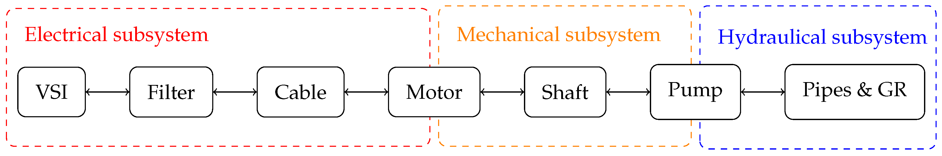
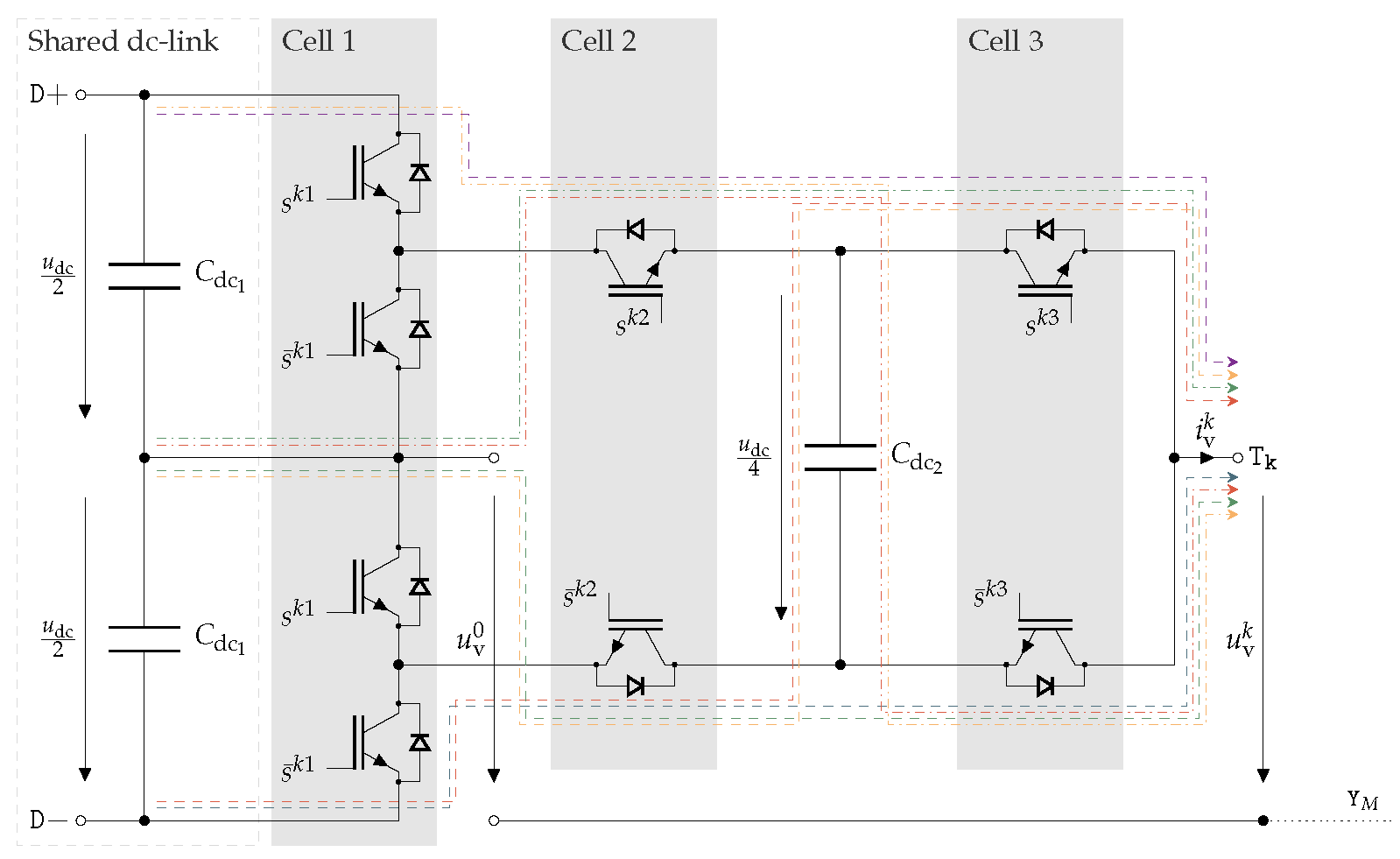
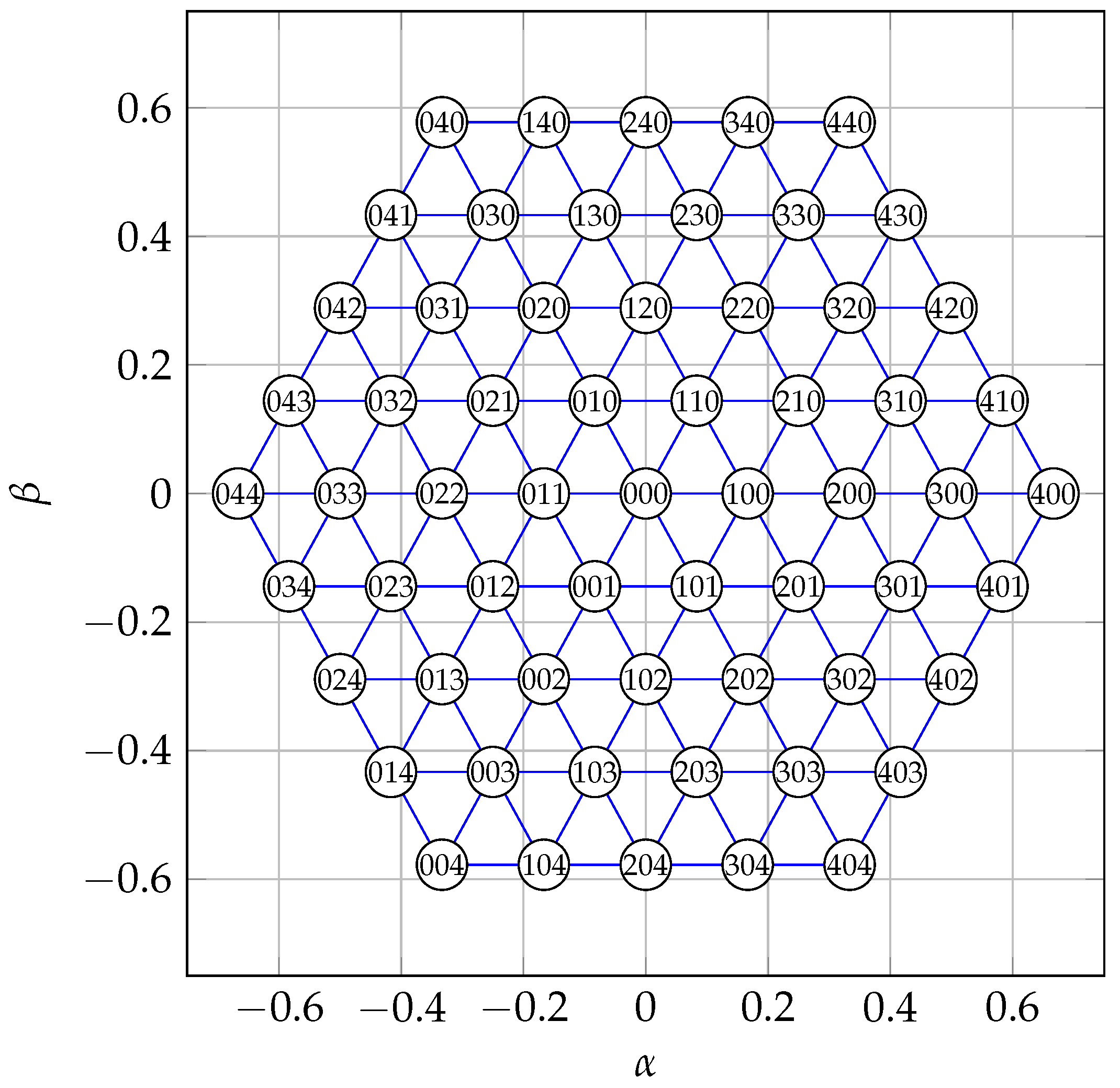
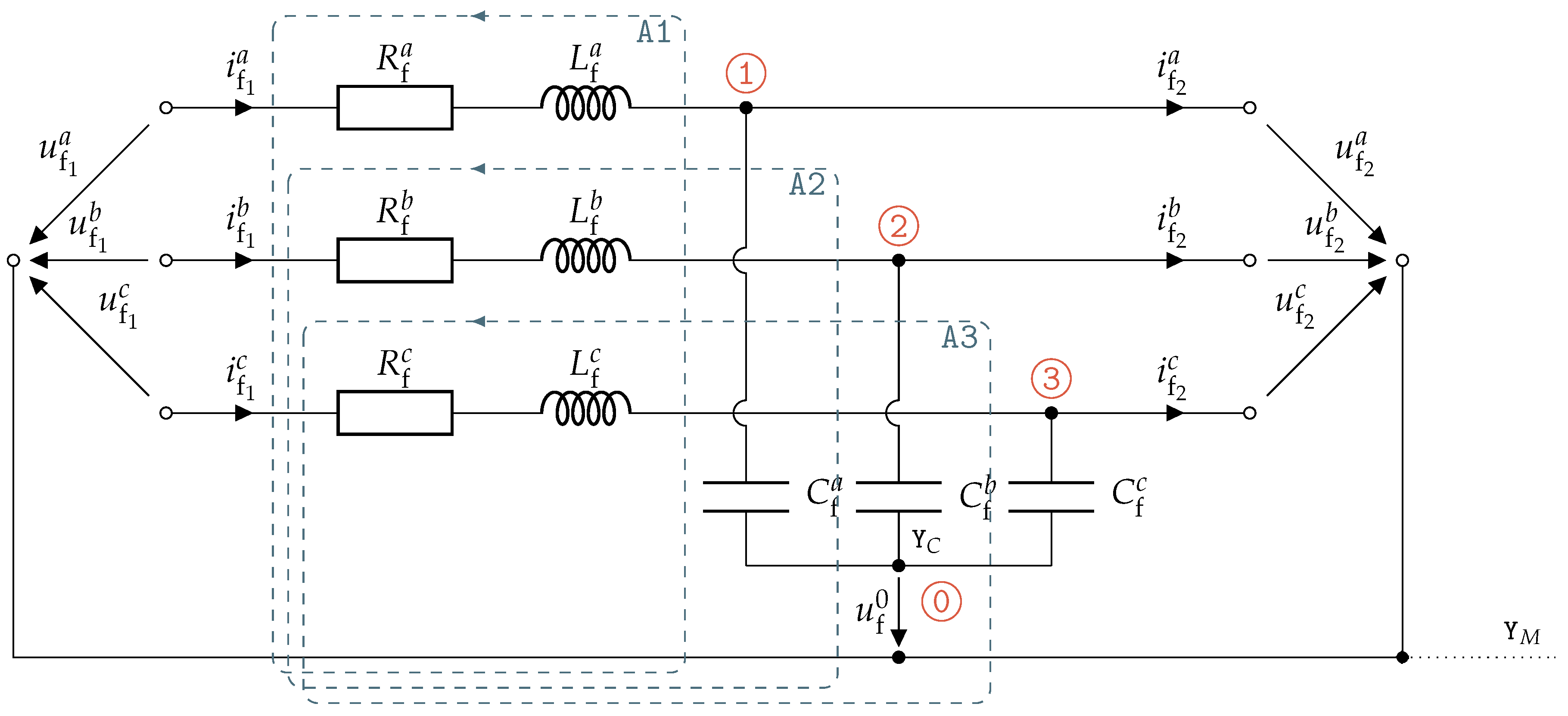
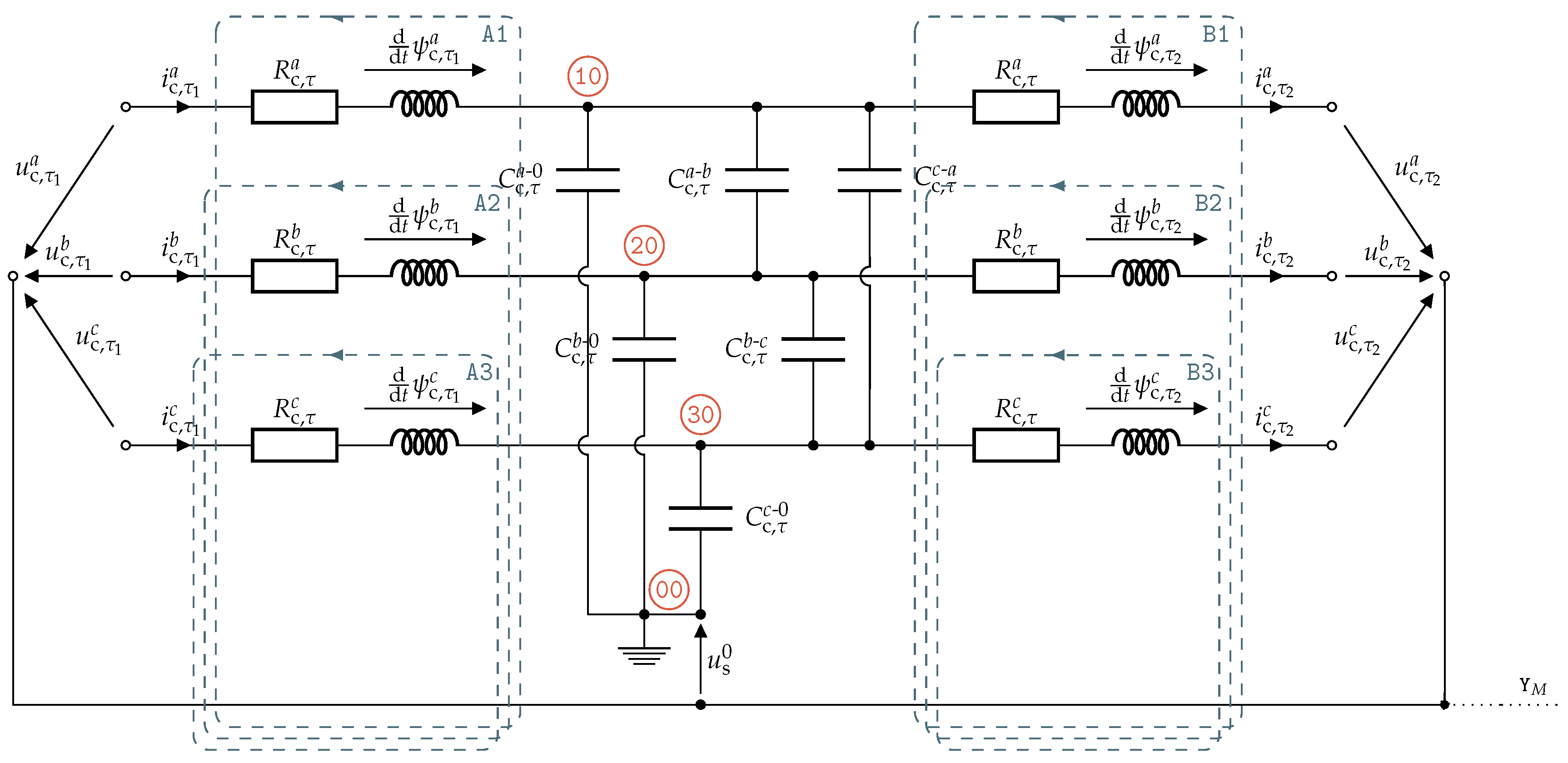
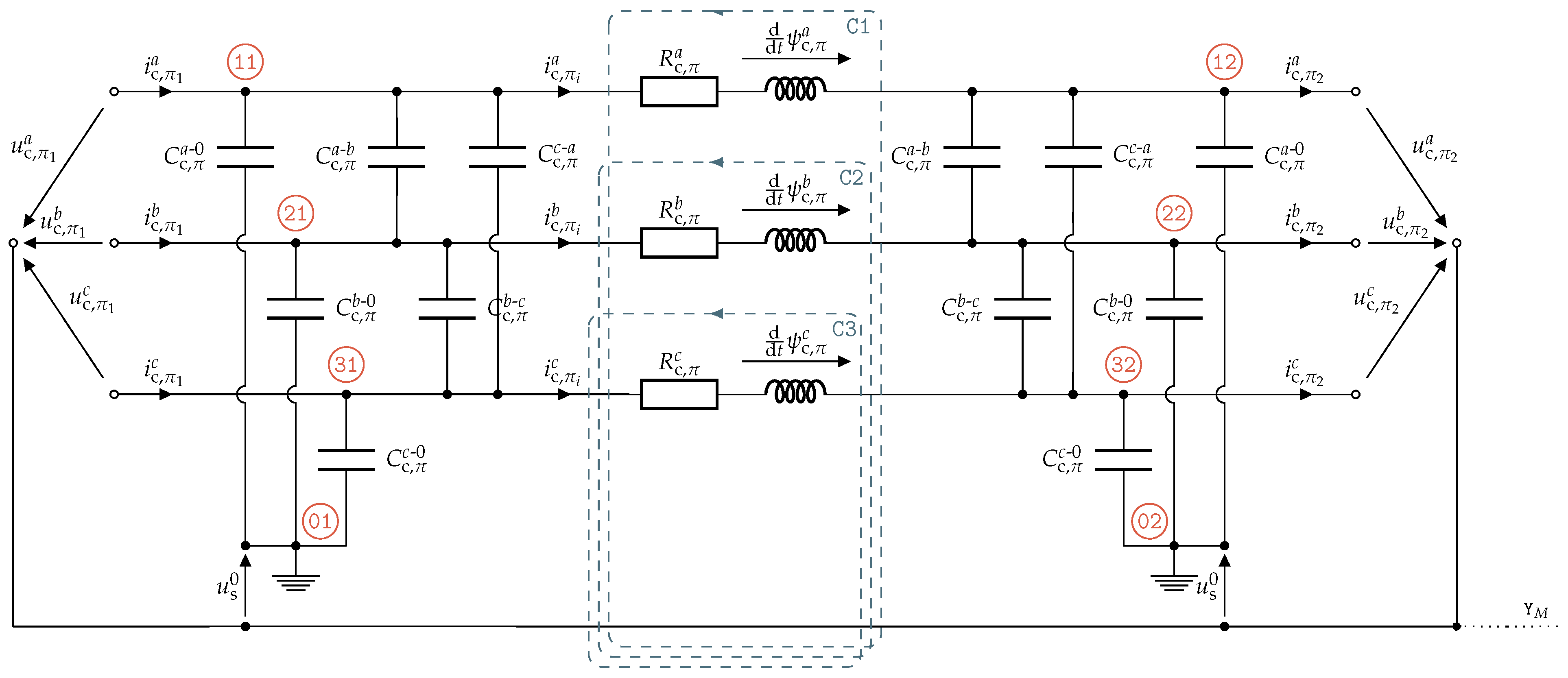
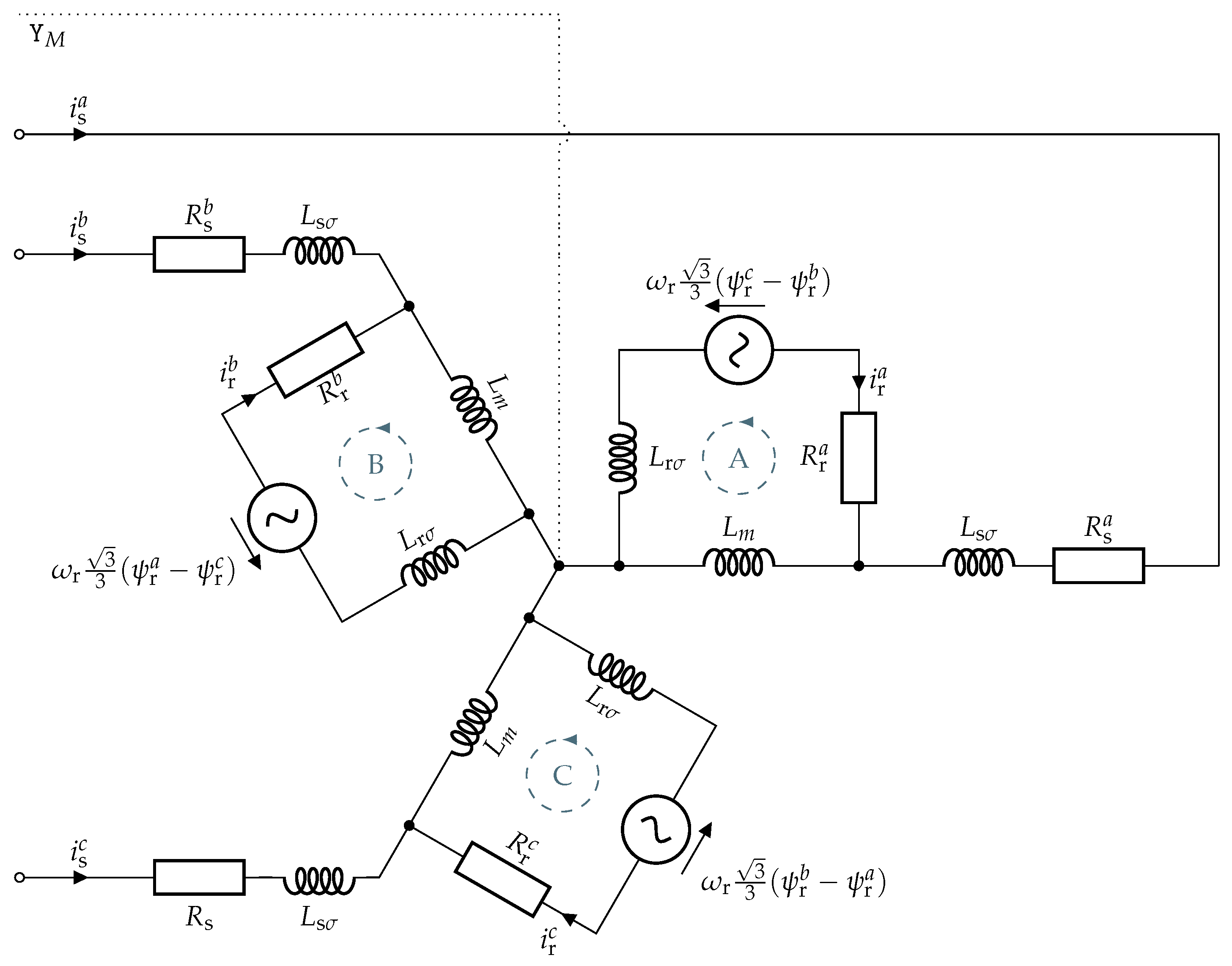
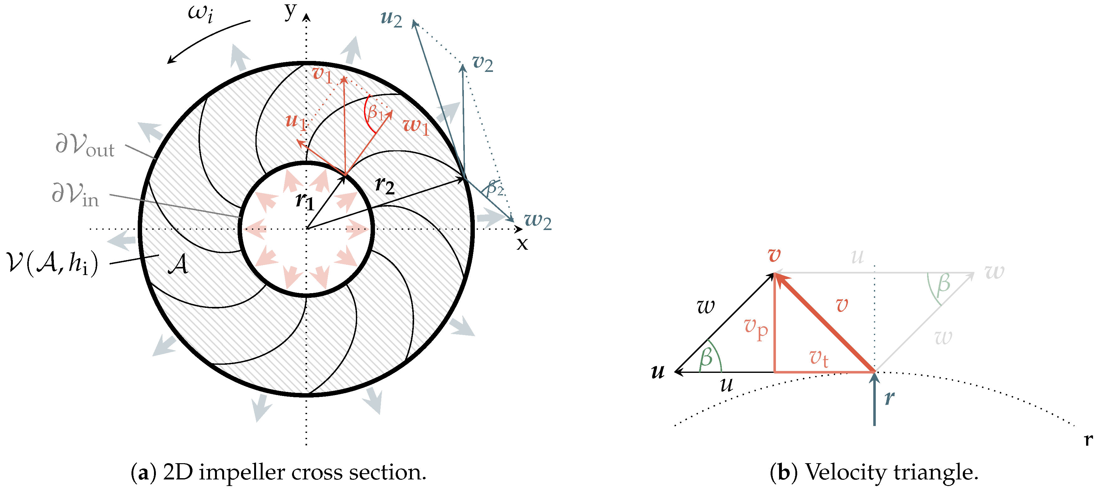
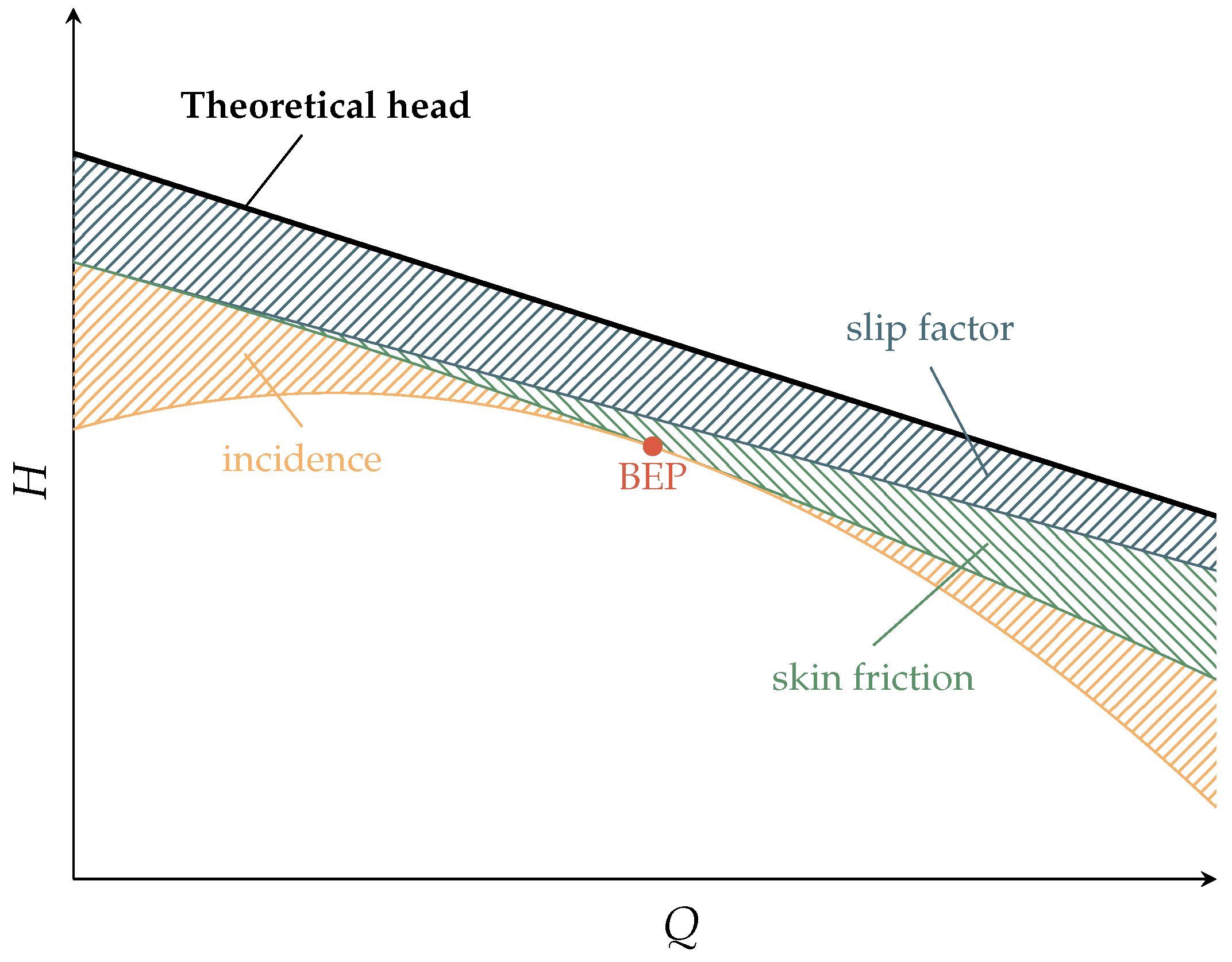
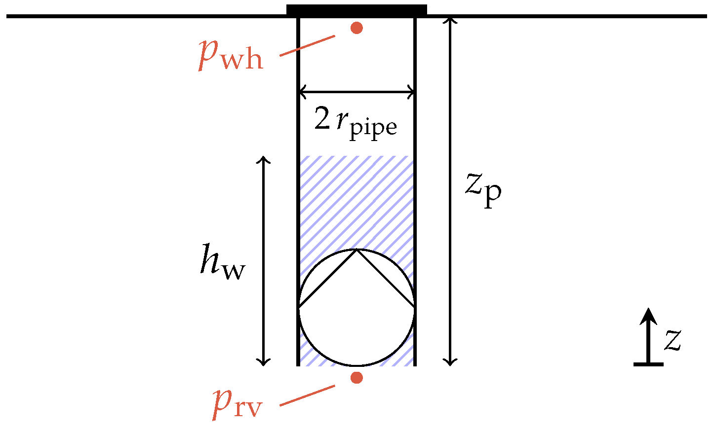
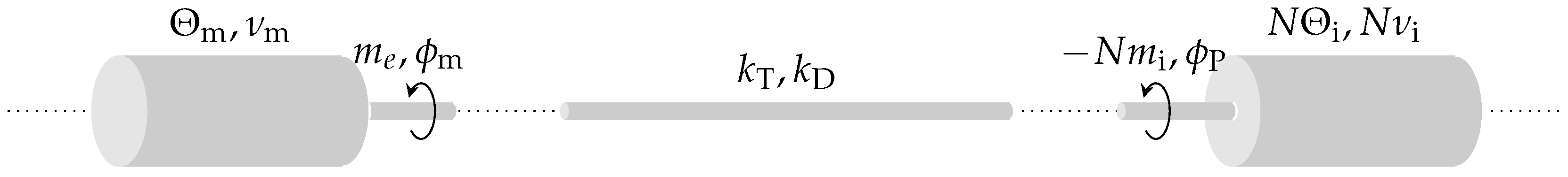
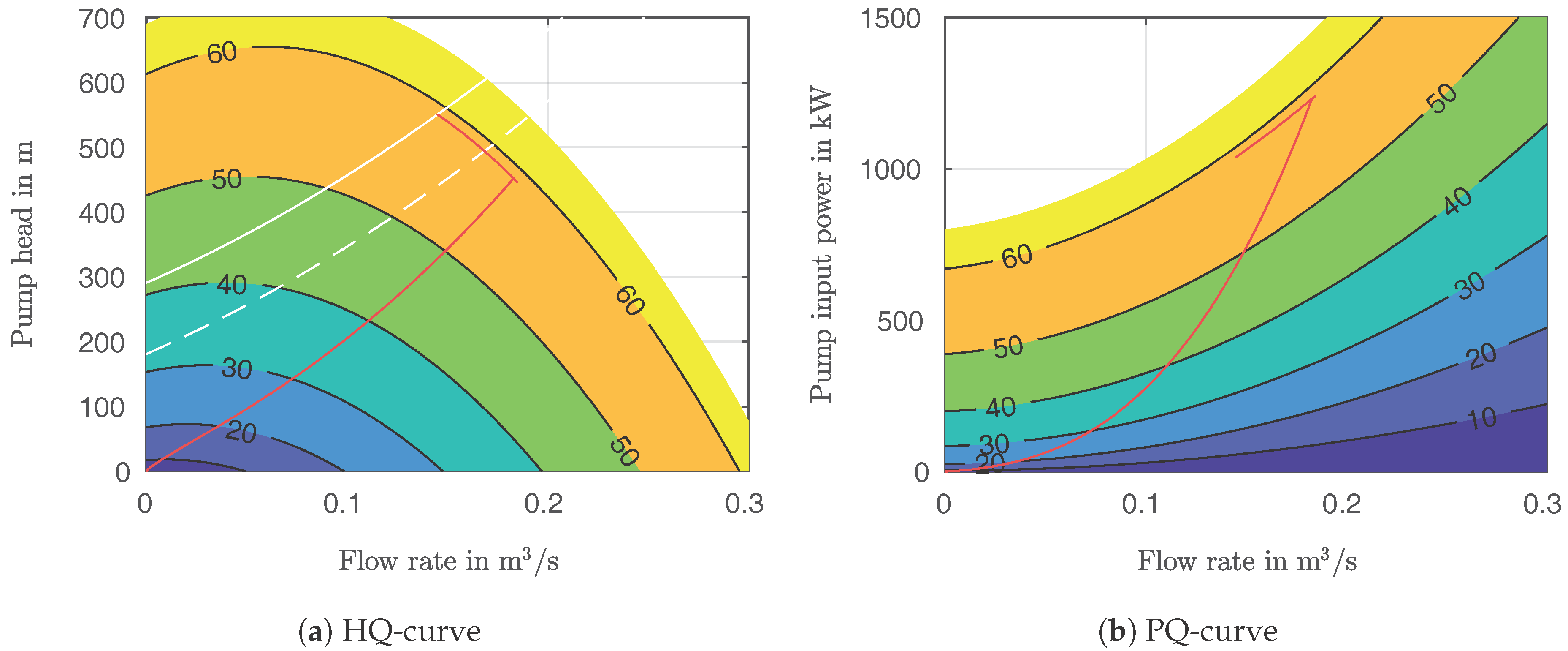
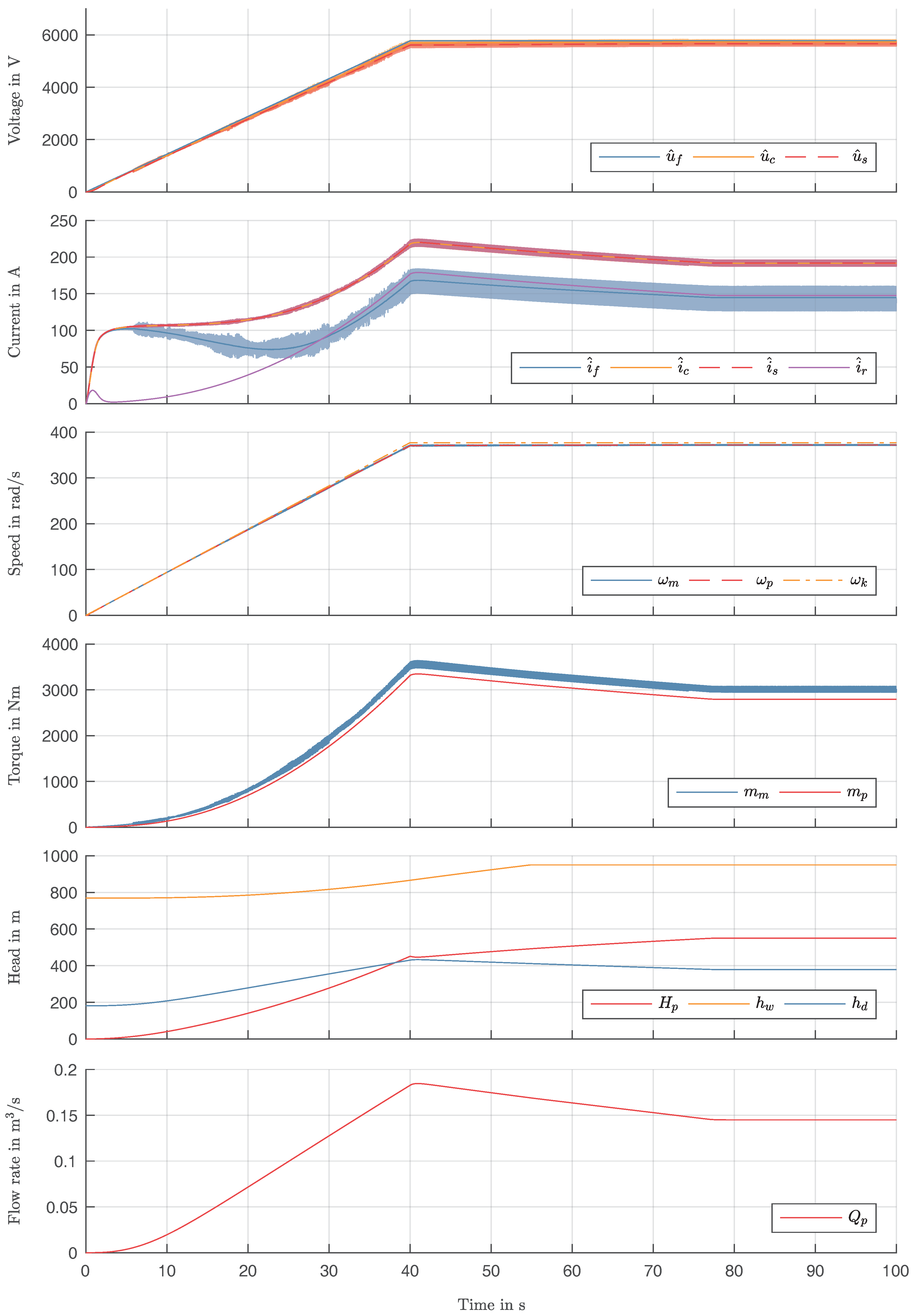
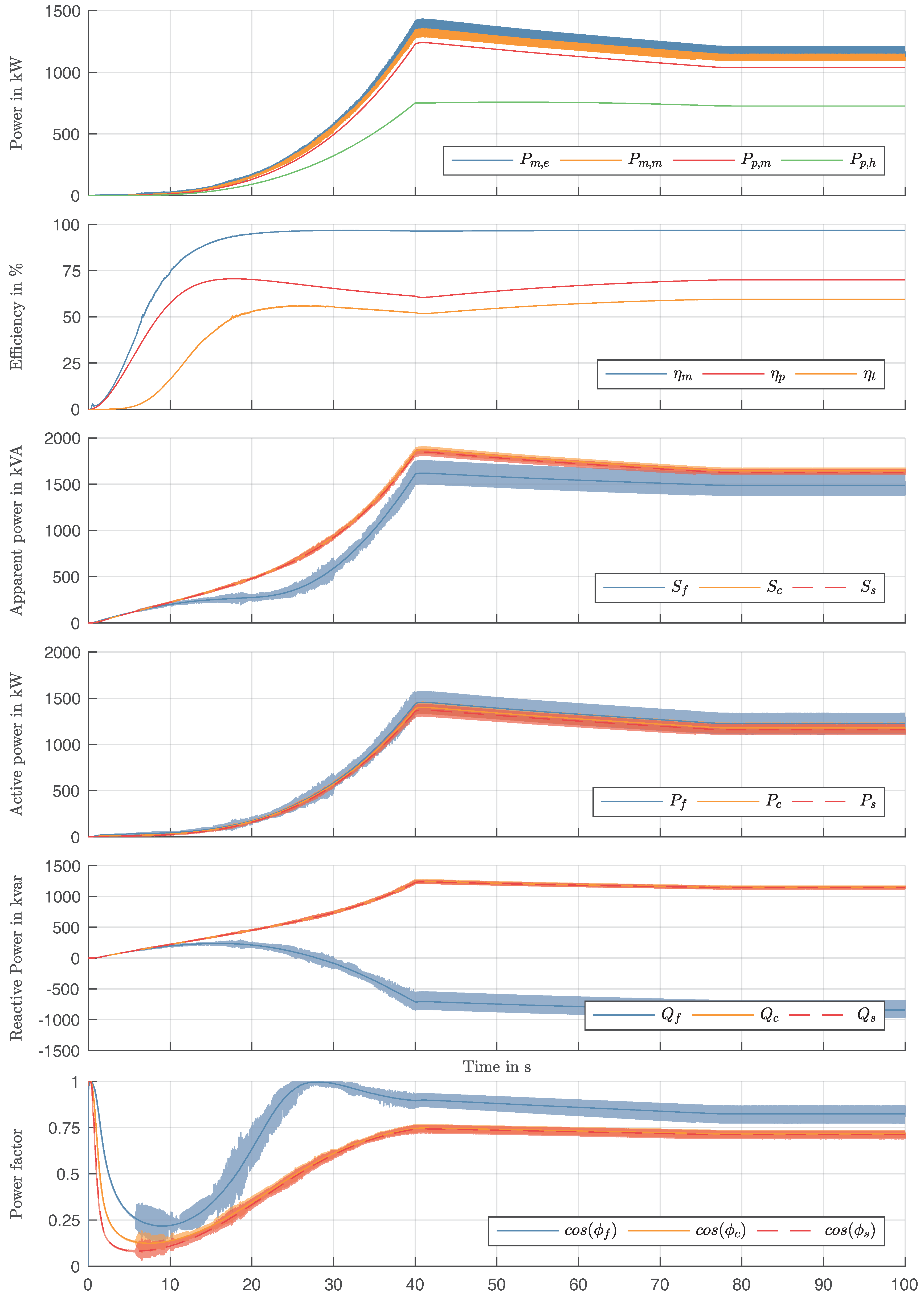
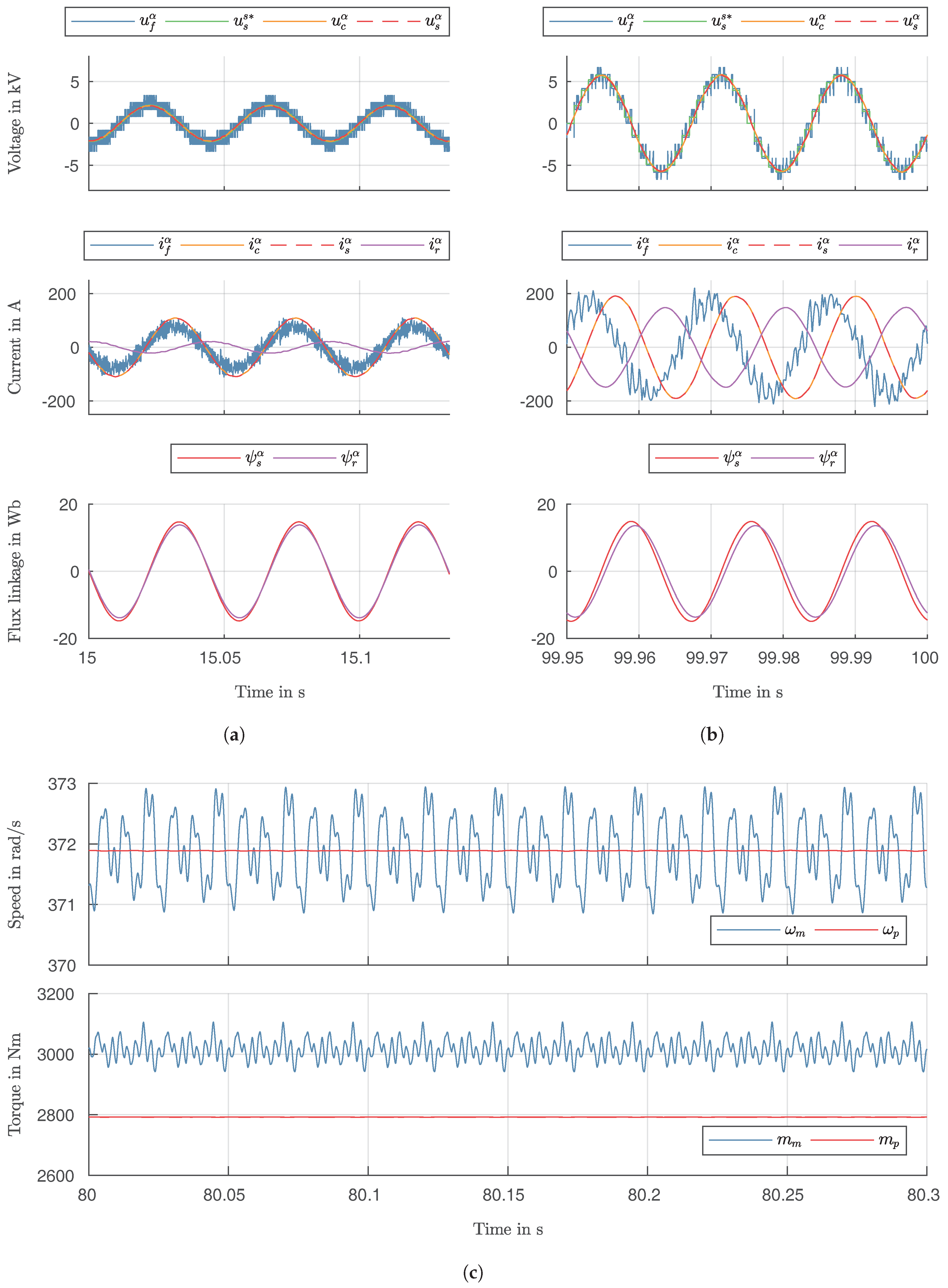
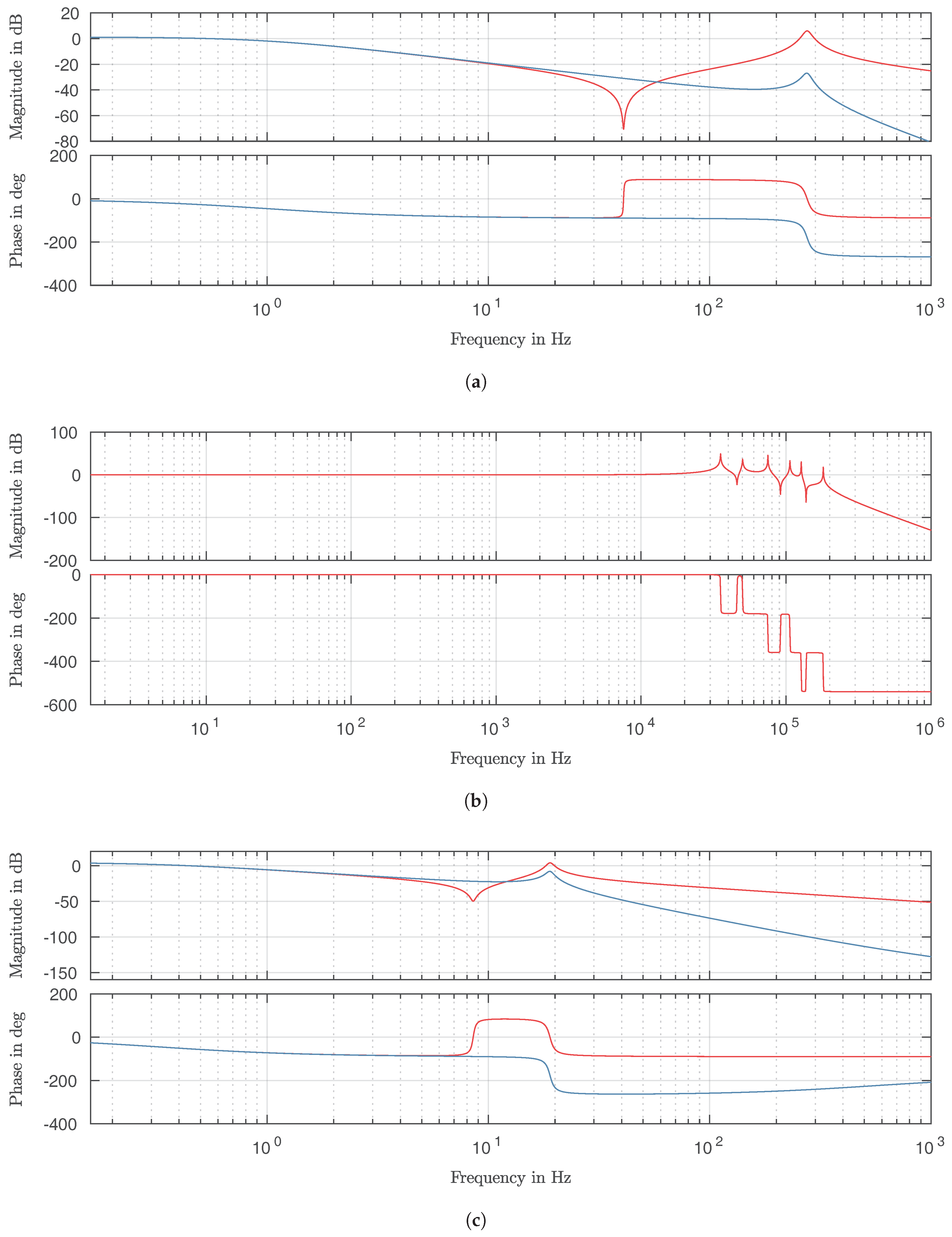
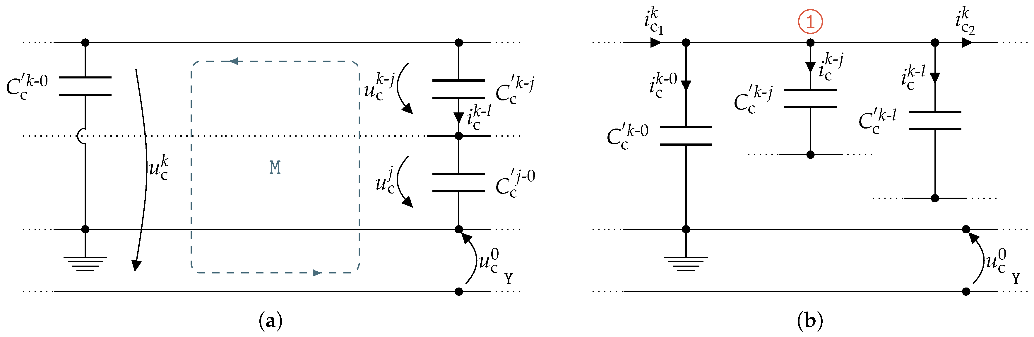
Table 1.
Switching states and output voltage levels of a single 5-level ANPC inverter phase.
| State | Switch | Switch | Switch | Output Voltage |
|---|---|---|---|---|
| 0 | 0 | 0 | 0 | |
| 1 | 0 | 0 | 1 | |
| 1 | 0 | 1 | 0 | |
| 2 | 1 | 0 | 0 | 0 |
| 2 | 0 | 1 | 1 | 0 |
| 3 | 1 | 0 | 1 | |
| 3 | 1 | 1 | 0 | |
| 4 | 1 | 1 | 1 |
Table 2.
Simulation parameters of the electrical subsystem.
| Parameter | Variable | Value | Unit | |
|---|---|---|---|---|
| Inverter | DC-link voltage | 10,000 | ||
| Switching frequency | 1000 | |||
| Filter | Filter inductance | 3.1 × 10⁻³ | ||
| Filter capacitance | 110 × 10−9 | |||
| Resonant frequency | 272.5 | |||
| Cable | Length | 997.5 | ||
| Line resistances | 0.38 × 10⁻³ | |||
| Line self inductances | 1.15 × 10⁻⁶ | |||
| Line mutual inductances | 0.86 × 10⁻⁶ | |||
| 0.69 × 10⁻⁶ | ||||
| Line self capacitances | 82.5 × 10⁻¹² | |||
| Line mutual capacitances | −32.2 × 10⁻¹² | |||
| −32.2 × 10⁻¹² | ||||
| Motor | Rated voltage (phase-peak) | 5750 | ||
| Rated current (phase-peak) | 190 | |||
| Number of pole pairs | 1 | |||
| Stator resistance | 0.37 | |||
| Rotor resistance | 0.47 | |||
| Main inductance | 129.5 × 10⁻³ | |||
| Stator leakage inductance | 8.7 × 10⁻³ | |||
| Rotor leakage inductance | 11.5 × 10⁻³ |
Table 3.
Simulation parameters of the mechanical subsystem.
| Parameter | Variable | Value | Unit | |
|---|---|---|---|---|
| Shaft | Torsion constant | 670 | ||
| Damping factor | 0.196 | |||
| Motor | Moment of inertia | 0.059 | ||
| Viscous friction coefficient | 1.5 × 10⁻³ | |||
| Pump | Moment of inertia | 0.233 | ||
| Viscous friction coefficient | 1.5 × 10⁻³ |
Table 4.
Simulation parameters of the hydraulic subsystem.
| Parameter | Variable | Value | Unit | |
|---|---|---|---|---|
| Pump | Number of pump stages | N | 28 | |
| Head parameters (fitted) | 0 | |||
| −5.27 × 10² | ||||
| 1.674 × 10⁻¹ | ||||
| 1.92 × 10⁻⁴ | ||||
| Torque parameters (fitted) | 0 | |||
| 1.686 × 10³ | ||||
| 2.237 × 10⁻¹ | ||||
| 5.579 × 10⁻⁴ | ||||
| System | Fluid inertance (full load) | 3.082 × 10³ | ||
| Required wellhead pressure | 10 × 10−5 | |||
| Setting depth | 950 | |||
| Pipe radius | 0.1 | |||
| Darcy factor | 0.12 | |||
| Reservoir pressure (idle) | 70 × 105 | |||
| Reservoir production index | 8.06 × 10⁻⁸ | |||
| Ambient and water | ||||
| temperature | 140 |
© 2017 by the authors. Licensee MDPI, Basel, Switzerland. This article is an open access article distributed under the terms and conditions of the Creative Commons Attribution (CC BY) license (http://creativecommons.org/licenses/by/4.0/).
Share and Cite
MDPI and ACS Style
Kullick, J.; Hackl, C.M. Dynamic Modeling and Simulation of Deep Geothermal Electric Submersible Pumping Systems. Energies 2017, 10, 1659. https://doi.org/10.3390/en10101659
AMA Style
Kullick J, Hackl CM. Dynamic Modeling and Simulation of Deep Geothermal Electric Submersible Pumping Systems. Energies. 2017; 10(10):1659. https://doi.org/10.3390/en10101659
Chicago/Turabian StyleKullick, Julian, and Christoph M. Hackl. 2017. "Dynamic Modeling and Simulation of Deep Geothermal Electric Submersible Pumping Systems" Energies 10, no. 10: 1659. https://doi.org/10.3390/en10101659
Note that from the first issue of 2016, this journal uses article numbers instead of page numbers. See further details here.