A Maximum Power Transfer Tracking Method for WPT Systems with Coupling Coefficient Identification Considering Two-Value Problem


College of Automation, Chongqing University, Chongqing 400044, China
*
Author to whom correspondence should be addressed.
Energies 2017, 10(10), 1665; https://doi.org/10.3390/en10101665
Submission received: 4 September 2017
/
Revised: 4 October 2017
/
Accepted: 12 October 2017
/
Published: 20 October 2017
(This article belongs to the Special Issue Wireless Power Transfer and Energy Harvesting Technologies)
Abstract
:Maximum power transfer tracking (MPTT) is meant to track the maximum power point during the system operation of wireless power transfer (WPT) systems. Traditionally, MPTT is achieved by impedance matching at the secondary side when the load resistance is varied. However, due to a loosely coupling characteristic, the variation of coupling coefficient will certainly affect the performance of impedance matching, therefore MPTT will fail accordingly. This paper presents an identification method of coupling coefficient for MPTT in WPT systems. Especially, the two-value issue during the identification is considered. The identification approach is easy to implement because it does not require additional circuit. Furthermore, MPTT is easy to realize because only two easily measured DC parameters are needed. The detailed identification procedure corresponding to the two-value issue and the maximum power transfer tracking process are presented, and both the simulation analysis and experimental results verified the identification method and MPTT.
1. Introduction
Wireless power transfer (WPT) has made a great development in the past few decades. It has been used in many occasions without the direct electrical contact (e.g., smart phone charging, implantable device charging, and electric vehicle (EV) charging, etc.) [1,2,3,4,5,6,7,8]. In a practical WPT application, usually the windings of the primary side and secondary side are compensated to degrade the input VA rating and improve the output power capacity [9,10,11]. Usually the operation frequency is designed to be the same with the natural frequency of the compensating resonant network to reduce the EMI [12,13]. However, one feature about the WPT system is that the load characteristic and the mutual inductance can affect the resonant frequency, so the power transfer capability and the system efficiency will be influenced accordingly [14,15].
Maximum power transfer (MPT) is an important performance index of WPT system, which can indicate the maximum power transfer capacity [1,16]. Traditionally, impedance matching method is utilized to realize the maximum power transfer tracking (MPTT) [17]. Reference [18] realizes the impedance matching by adding passive components while references [5,19,20,21] do the impedance matching through DC/DC converters (e.g., Boost, Buck, Sepic, etc.). Since the load resistance of a practical WPT system varies with time, therefore using DC/DC converters to do the impedance matching is more suitable for the frequent load variations [19]. However, one thing about the impedance matching using DC/DC converters is that it cannot be realized when unknowing the parameters, such as coupling coefficient and load resistance [22,23]. Therefore, in order to achieve MPTT, the identification of these changing parameters is needed previously.
Some researchers have done the related works on the load and coupling coefficient identification. Reference [14] presents a coupling coefficient and load identification method, with two equations derived by switching the compensation capacitors, the two variables can be calculated. However, the equations require the information of the resonant currents on primary and secondary sides, which will increase the difficulty in practice. References [22,23] present a dynamical identification method of coupling coefficient, and it only need to measure the parameters on the secondary side. However, it needs to measure the RMS value of alternating currents, which will bring harmonic interference. In addition, the continuous and discontinuous operation modes will influence the accuracy of the modeling. Reference [24] also studies the identification of mutual inductance and load resistance. These two parameters can be calculated under one operating frequency condition with the front-end monitoring method. However, the high estimation accuracy will sacrifice the system efficiency.
This paper presents an identification method of coupling coefficient for MPTT in WPT system. The method does not require any other circuit to implement the identification and the identification only need to measure two DC parameters on secondary side. Especially, the two-value issue during the identification process is solved. As long as the coupling coefficient and load are determined, the maximum power transfer tracking is realized by impedance matching. The paper is structured as follows: system topology, coupling coefficient identification, and MPTT description is presented in Section 2, system parameters and the simulation analysis are shown in Section 3, experimental verification of the proposed coupling coefficient identification and the MPTT are shown in Section 4, and the conclusions are presented in Section 5.
2. Coupling Coefficient Identification and Maximum Power Transfer Tracking
2.1. System Topology
Figure 1 shows the schematic circuit of the proposed tracking topology, where the input DC voltage is given by E, Rb is the load resistance. Rp and Rs are the internal resistance of Lp and Ls, respectively. Lp, Cp constitute the primary series resonant circuit, while Ls, Cs constitute the secondary series resonant circuit. M is the mutual inductance, and satisfies (k represents the coupling coefficient). S1~S4 constitute the full-bridge inverter, while D1~D4 constitute the rectifier. Sb, Db, Lb, Cb constitute the Buck converter. Rbin and Rrin are the equivalent input impedances of the Buck converter and rectifier circuit, respectively. ip and is are the resonant currents. Vs, Vr, Ub are the input voltage of the resonant circuit, the rectifier and the Buck converter respectively. To reduce EMI, assuming the operating frequency f of the inverter is same with the nature frequency of the resonant circuit, i.e., .
2.2. Identification of the Coupling Coefficient
Assuming that there is no power loss in the rectifier, the relationship between the input and output resistance is:
As for the relationship between the input and output resistance of the Buck converter, it can also be derived. Take the continuous conduction mode (CCM) operation of Buck converter into consideration, the relationship between Rbin and Rb is:
where d indicates the duty cycle of the Buck converter, and d should satisfy: to achieve the CCM operation of Buck converter. Rb can be derived by .
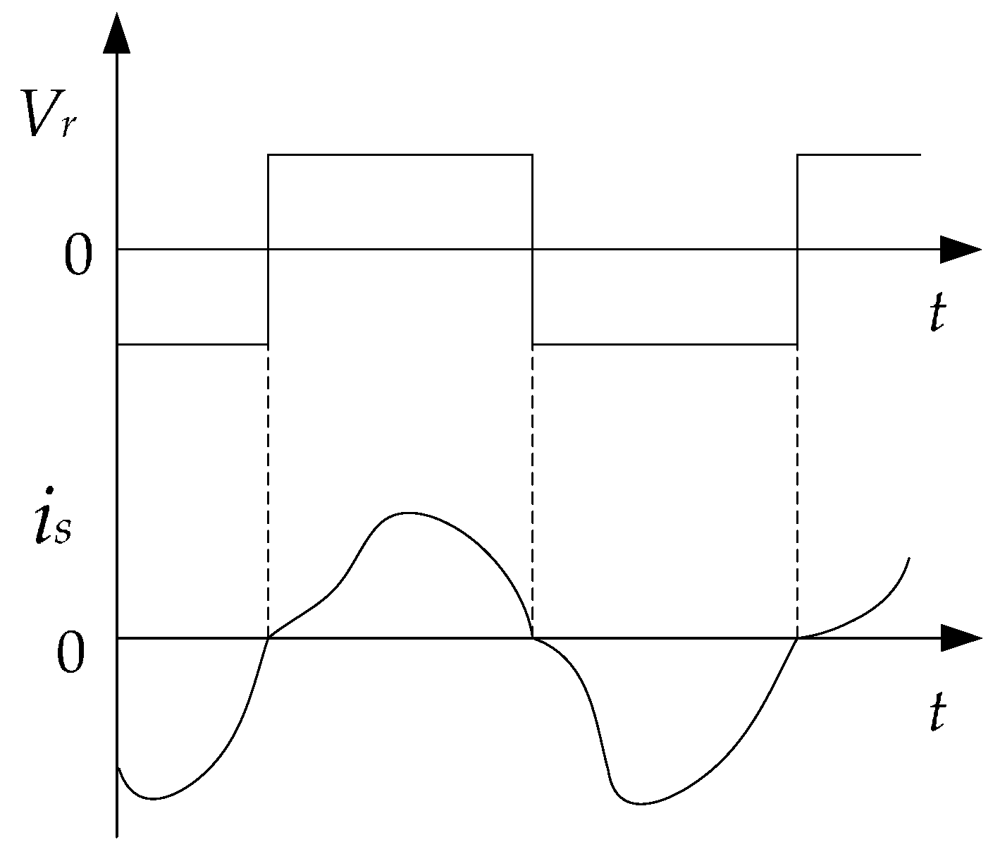
It is found that the theoretical model of the secondary circuit (i.e., resonant circuit, rectifier, and Buck converter) is more precisely when the secondary resonant current is is continuous. Figure 2 is presented to show a case of continuous current. is is continuous with the following condition [25]:
where ω is the angular frequency of the resonant circuits, and satisfies .
By calculating Equations (1) and (2), the following relationship can be derived:
The RMS value of ip is:
where Us is the RMS value of Vs satisfying . Zref is the reflected impedance, satisfies .
The RMS value of Vr is:
Therefore, the output voltage Uo can be calculated as:
By calculating (7), the relationship between k and the measured Uo can be derived as:
E, ω, d, Lp, Ls, Rp, and Rs are the known parameters. k can be calculated from (8) with the measured DC parameters Uo and Io. However, Equation (8) shows that derivation of k may have two values based on one instance of Uo. Therefore, at least two instances of output voltage are needed to identify the actual k. In the next part, this two-value issue during the identification will be solved.
2.3. Dealing with the Two-Value Issue When Identifing the Coupling Coefficient
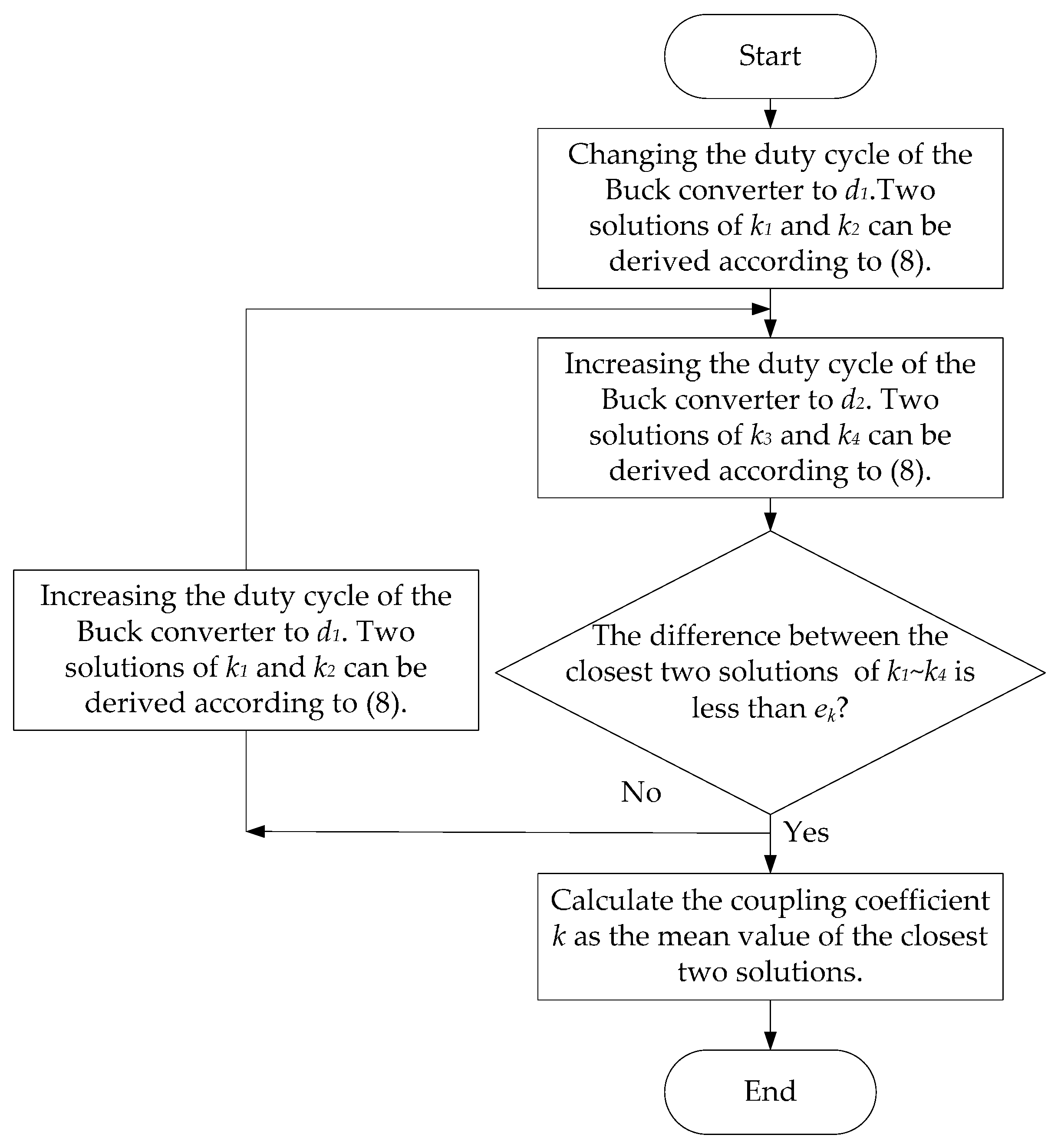
Figure 3 is presented here to indicate the identification process when considering the two-value issue.
During the identification process, by changing the duty cycle twice, two instances of Uo can be derived. By calculating Equation (8), four solutions of coupling coefficient can be obtained. Then compare the four solutions if there is a difference between two solutions is less than the tolerance error ek. The actual coupling coefficient can be determined by calculating the mean value of these two solutions. Otherwise, we will increase the duty cycle and restart the identification process. It should be noted that we just need the identification of the coupling coefficient once before the maximum power tracking process when there is no relative movement between the primary and secondary coils. When the coupling coefficient is identified, the maximum power tracking can be achieved through impedance matching and this will be introduced in the following section.
2.4. Maximum Power Transfer Tracking
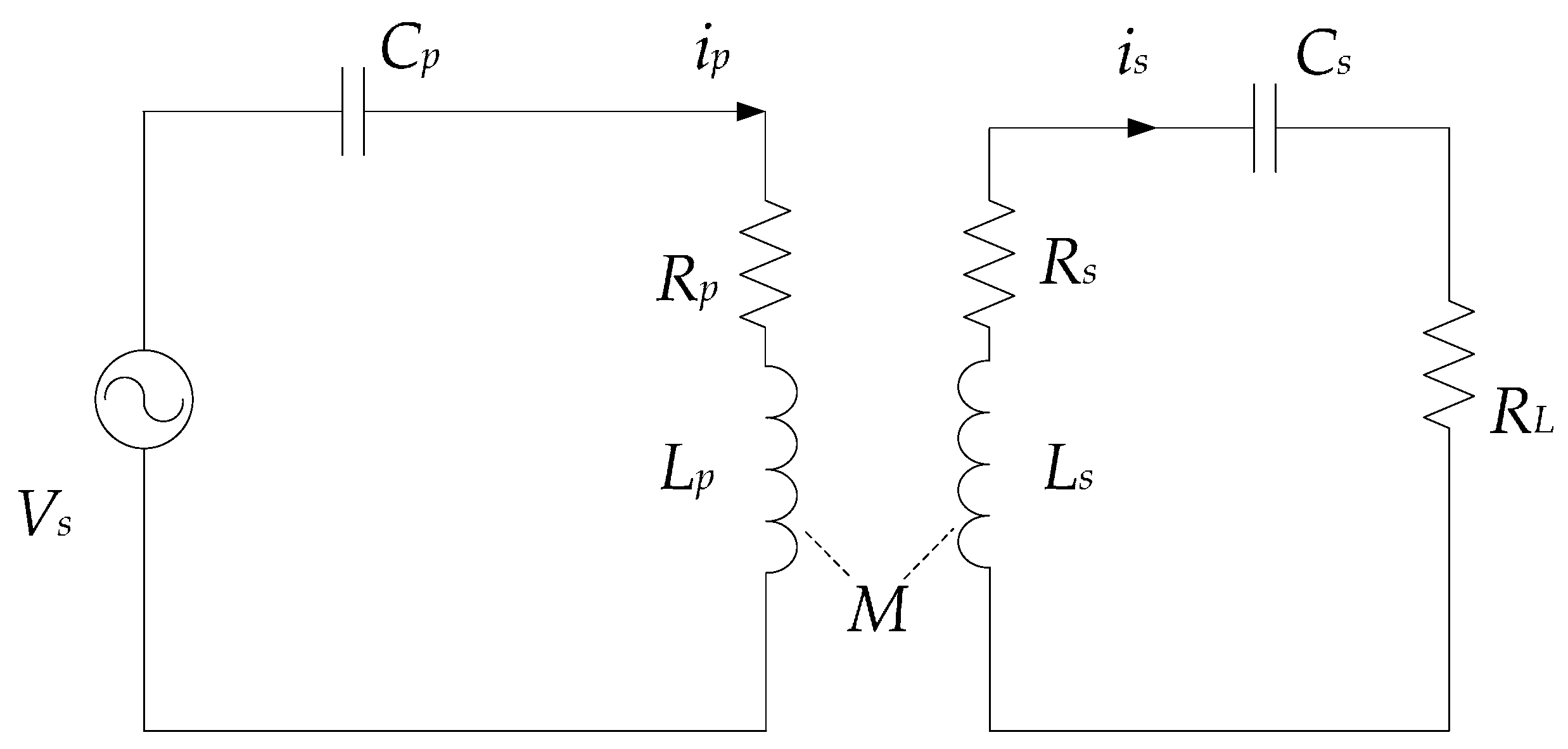
Take a series-series (SS) topology WPT system shown in Figure 4 as example. The coupling equations can be derived as:
where and . When the operating frequency equals to the natural frequency of the resonant circuits (i.e., Xp = 0; Xs = 0), the output power PL can be derived as:
where, Is is the RMS value of is, Us is the RMS value of Vs.
The maximum power transfer point corresponding to the load resistance can be solved by , the optimum resistance is:
The maximum output power is:
System efficiency (given by the output power divided by input power) at the maximum power transfer point is:
where Ip is the RMS value of ip.
As is mentioned before, the load resistance of the WPT system may change during the whole power transfer process, and the transferred power will change accordingly. As the tracking topology shown in Figure 1, a Buck converter is utilized to track the maximum power point. MPTT can be realized through changing the duty cycle of the Buck converter. By calculating Equations (4) and (11), the optimum duty cycle dopt can be derived:
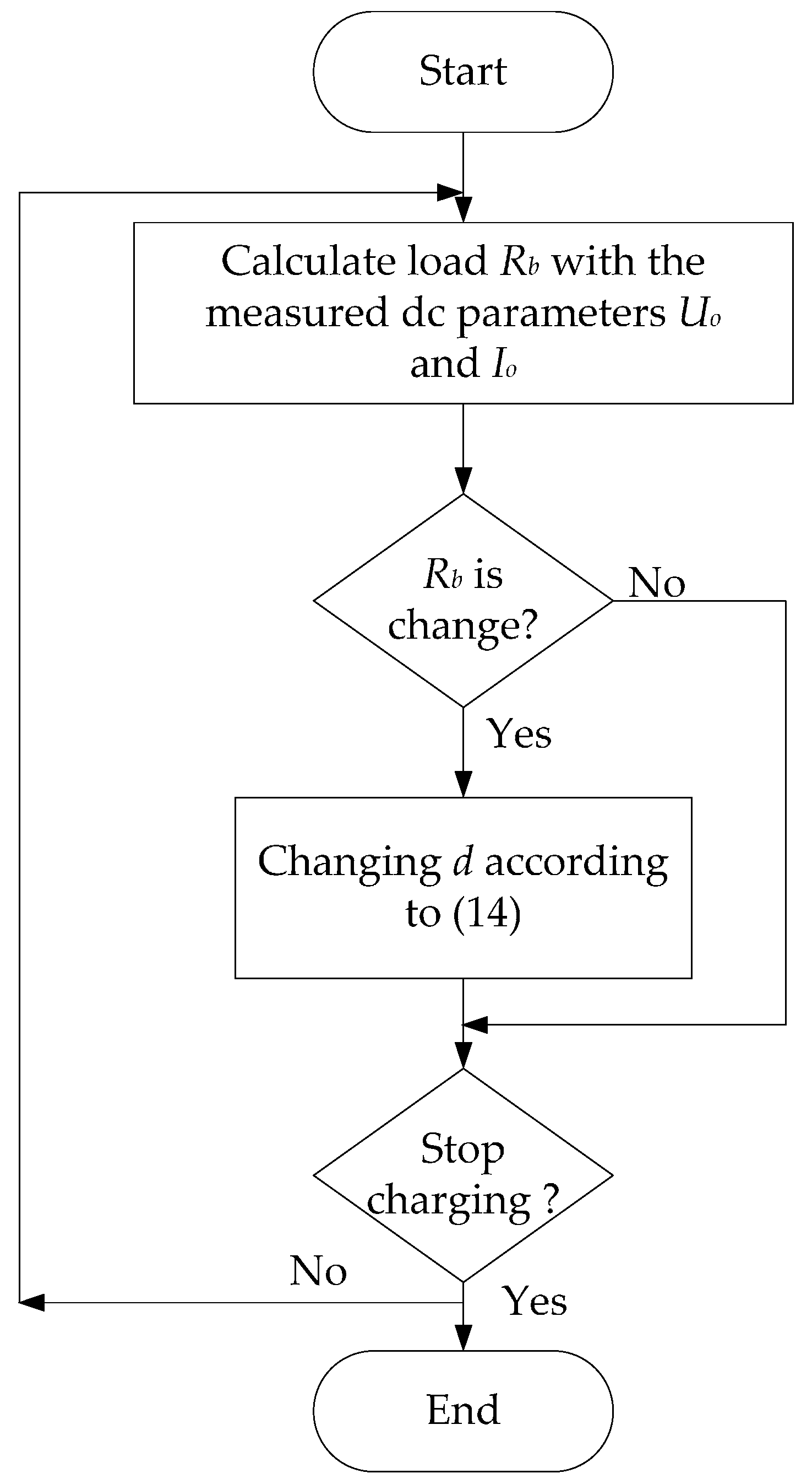
Figure 5 shows the flowchart of the maximum power transfer tracking process. After the identification of the coupling coefficient and the load resistance, MPTT can be realized through impedance matching (i.e., changing the duty cycle of the Buck converter). Load Rb is detected during the whole charging process. If Rb is varied, the optimum duty cycle d derived by Equation (14) will fed to the Buck converter.
3. Simulation Analysis
3.1. System Parameters and the Control Structure
In this section, the presented identification approach and MPTT will be verified by Matlab/Simulink. With the parameters shown in Table 1 and the topology shown in Figure 1, a simulation model is built. The parameters of the Litz-wire coils indicate the item used in experiment. fb is the frequency of the Buck converter.
Figure 6 shows the control structure diagram. The detection unit detects the DC output voltage and current on the secondary side. The controller identifies the coupling coefficient and control the duty cycle of the Buck converter to track the maximum power.
3.2. Analysis of the Coupling Coefficient Identification and Maximum Power Transfer Tracking
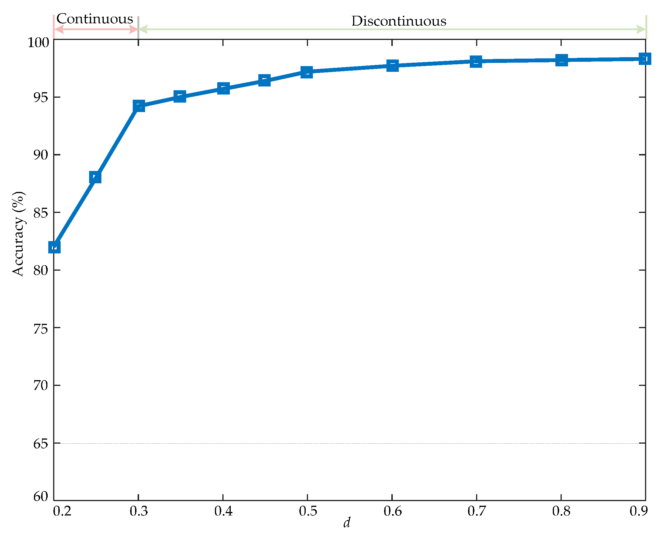
As mentioned before, the theoretical model of the secondary side circuit will be more precise when is is continuous. According to Equation (3) and the parameters shown in Table 1, we can derive that when d is larger than 0.3, the current is continuous. Figure 7 shows the identification accuracies of the coupling coefficient when d varies from 0.2 to 0.9. The reference k is selected as 0.15 while Rb = 10 Ω.
Figure 7 shows that when d is larger than 0.3 (i.e., is is continuous), the identification accuracies are all larger than 95%, while the identification accuracies are below 90% when is is discontinuous. Therefore, only the continuous current case is taken into consideration in this paper.
Table 2 shows the coupling coefficient identification results when the reference k varies, where the load resistance Rb is set at 10 Ω, d1 = 0.5, d2 = 0.6, ek = 0.0027. The identification accuracy is over 94% at all of the coupling coefficient conditions. These high accuracy identification results indicate that the identification method is feasible.
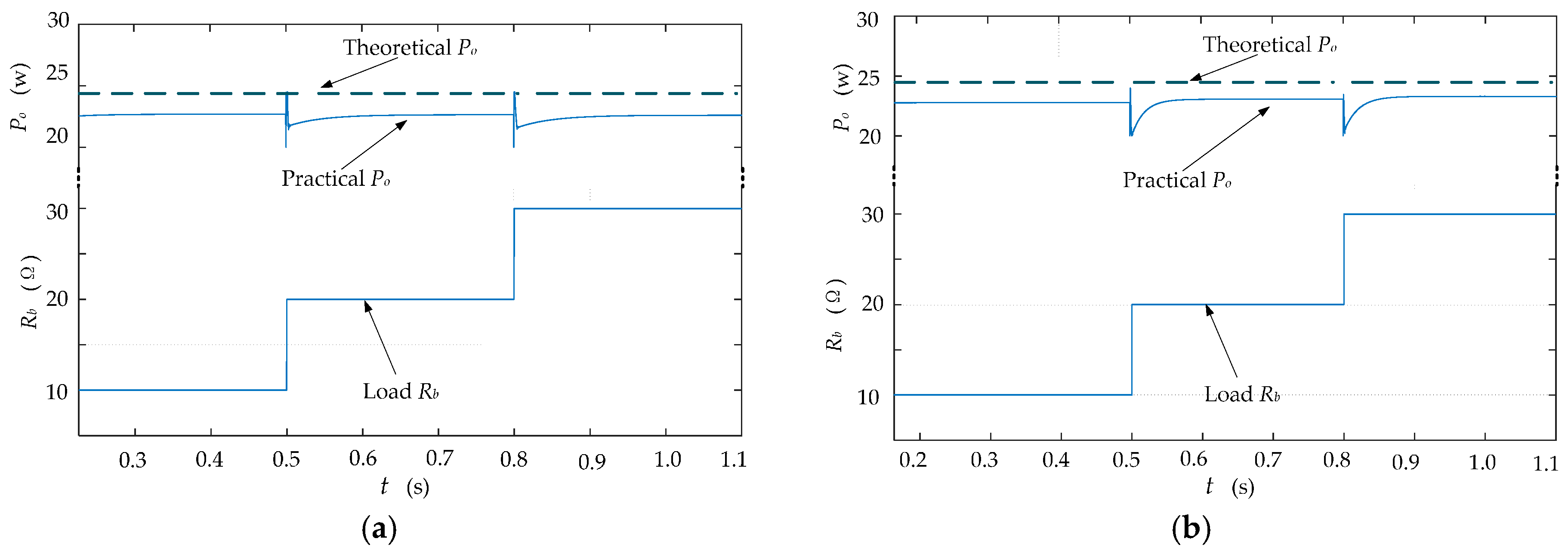
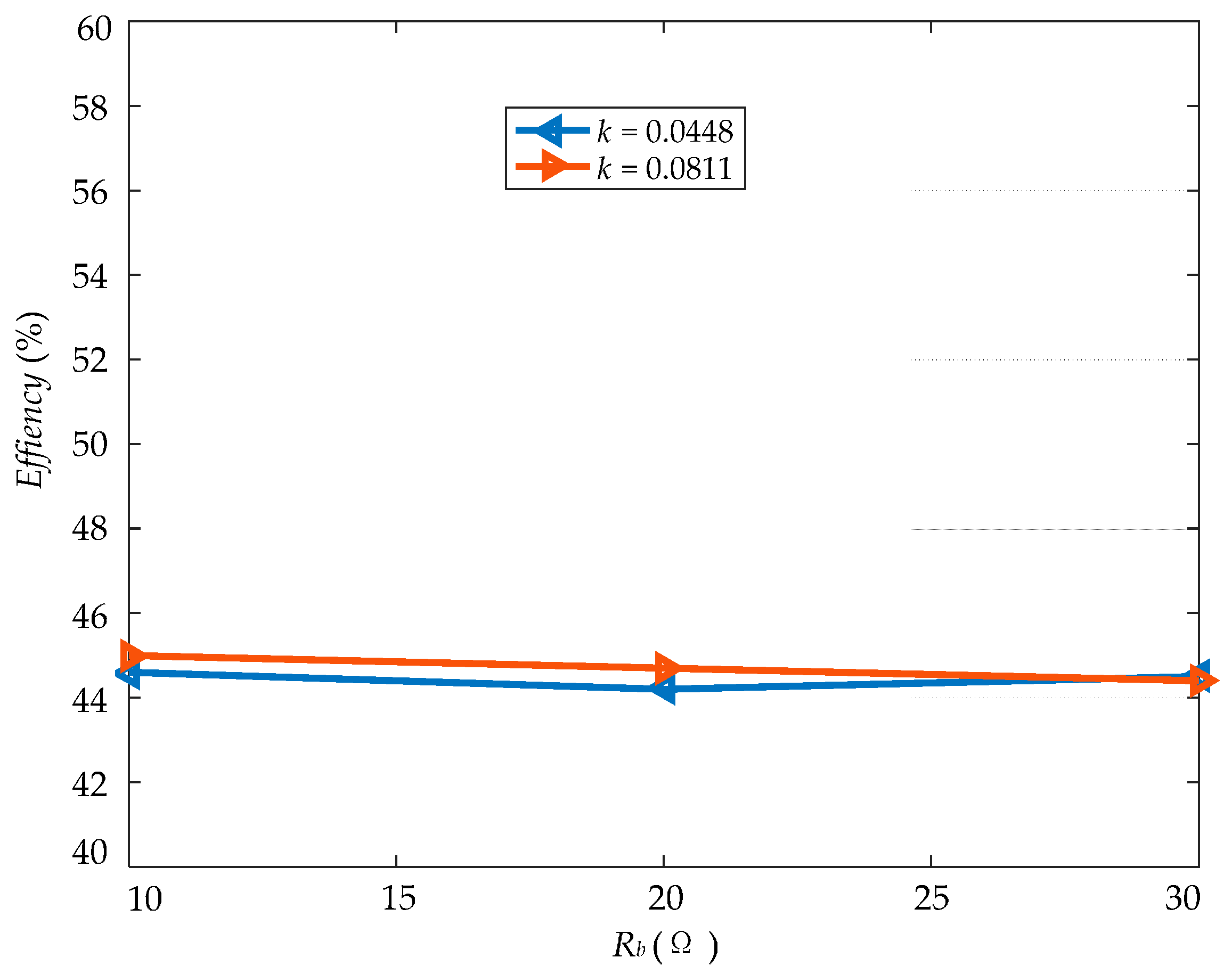
As for the MPTT of the system, the simulation results are shown in Figure 8. Rb changes from 10 to 30 Ω, and two coupling coefficient cases are considered (the given coupling coefficients are 0.0448 and 0.0811, while the identified coupling coefficients are 0.0474 and 0.0839). The theoretical maximum power can be derived from (12), which are shown in the top of Figure 8a,b with dot line. The middle of the figure indicates the practical output power while the load Rb variation is shown in the bottom of the figure. Both the two figures (a) and (b) share the similar features, due to the identification error of k and the non-ideal of the semiconductor switch and diode, the practical output power is slightly lower than the theoretical value. The steady state of the practical output power (Po) is almost the same at different load condition, this can prove that the maximum power tracking is achieved. At the changing instant of load Rb, the practical output power is pulsatile due to the switch noise, and it cannot be totally eliminated.
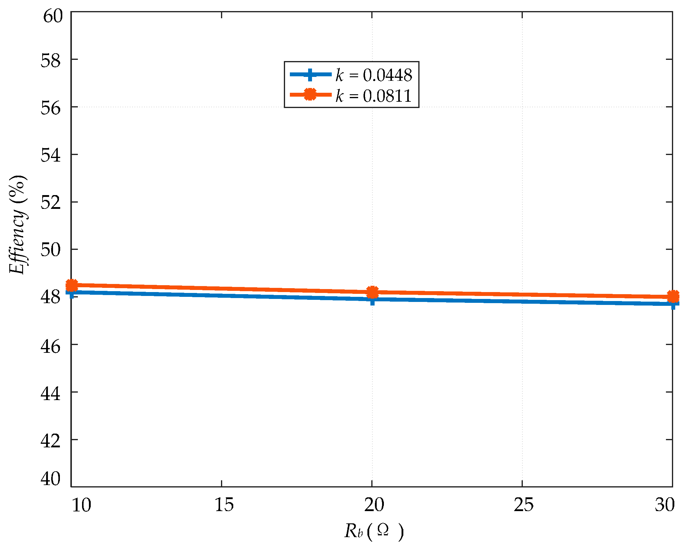
System efficiencies at steady state under these two coupling coefficients are shows in Figure 9. In general, the output power is at its maximum when the external resistance is equal to the internal resistance, so the efficiency under the maximum power transfer condition is close to 50%.
4. Experimental Analysis
4.1. Experimental Setup
An experimental setup is built to verify the proposal. The experimental system topology is same with Figure 1 and Table 1 gives its parameters. In the experiment, the primary and secondary coils are in same configuration and wound by Litz wires. The diameter of the coil is 14 cm, while the number of turns is 25. Figure 10 shows the photo of the experimental setup, where an ARM chip is used as the detection unit to measure the DC voltage and current, while an FPGA chip is selected as the controller. The variable load is achieved by switching the relay array.
4.2. Experimental Results
As is indicated before, k is firstly need to be identified before the maximum power tracking. Since there are two solutions with respect to one voltage Uo, as shown in Equation (8), so we need to motivate the system twice by changing d as shown in Figure 3. When there is difference lower than ek between two solutions, k can be calculated by averaging these two solutions. ek should be selected as a small value to ensure the high identification accuracy, in this paper we choose ek to be 0.0027 (i.e., the mutual inductance is 1 µH). One thing about the selecting of d is that, as can be seen from Figure 7, the identification accuracy is relatively higher when d is larger until d increase to a certain value. Therefore, when k cannot be identified, we just increase d as shown in Figure 3.
In order to verify the identification method of the coupling coefficient, we firstly measure two reference coupling coefficients under two alignment conditions of the coupling coils, the two values are 0.0811 and 0.0448 while the separation distance between the couplers are 6 cm and 9 cm, respectively. The identification process and the results are shown in Table 3.
As shown in Table 3, the identification of the two reference coupling coefficients 0.0811 and 0.0448 can be determined when d1 and d2 are selected as 0.5 and 0.6. k1 and k3 has the difference lower than ek, so the identification of k can be determined, and the accuracies of the two conditions are higher than 93%.
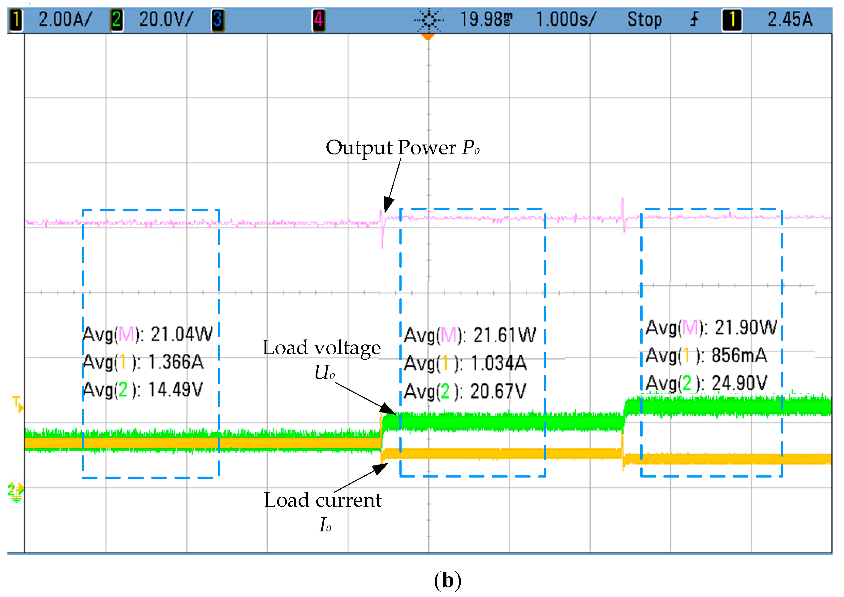
After the identification of k, MPTT can be achieved. We change the load resistance Rb at 10, 20, and 30 Ω. ARM chip can detect the load variation, and then the tracking duty cycle d can be calculated by Equation (14). The maximum power tracking results under the two coupling conditions are shown in Figure 11, where the values in the blue rectangular boxes indicate the measured output power Po, Io, and Uo under different load and coupling conditions.
The top of the figure shows the practical output power, while the bottom of the figure shows the detected voltage Uo and current Io. By comparing Figure 11a,b and Figure 8a,b the experimental output power is slightly smaller than the simulation results because of the identification error of k and the losses in the experiment system. When load Rb changes, the tracked maximum output power is almost the same at the steady state, this can prove that the maximum power tracking is achieved.
System efficiencies under the MPTT condition are shown in Figure 12. The results are less than that of simulation results, partly due to the disturbance in the experiment.
These experimental results verified the proposed identification approach and MPTT method. It should be noted that there are always some errors during the experimental measurements, thus the identification accuracy and the maximum power are lower than the simulation results, to further improve the experimental accuracy, the improved filtering algorithms and circuits can be used to reduce the measurement errors. Furthermore, the semiconductor switching loss is ignored when calculating the theoretical output power, so both the simulation and the experimental output power are lower than the theoretical results. Besides, in this paper, we just consider the variations of the load resistance, other variations of the system parameters are very small during the power transfer, so the interference is very small.
The coupling coefficient identification is required only once before the maximum power transfer tracking process when there is no relative movement between the primary and secondary couplers, and the required parameters are all in steady state. The identification time of the coupling coefficient is about 30 ms, while the detection time of Rb is about 10 ms in steady state. After the identification of k, the maximum power transfer tracking can be done through impedance matching. As for the changing of load Rb, the gap time between the two variable loads just need to be larger than the identification time. The proposed identification method shown in Figure 3 is also suitable for the dynamical identification of the coupling coefficient, and the variation of the coupling coefficient should be slower enough for the coupling coefficient identification.
5. Conclusions
This paper presents a maximum power transfer tracking method in WPT systems with coupling coefficient identification. A two instance determination method is given to prevent two-value issue during the identification. The identification algorithm is also presented in detail to realize MPTT. When compared with other identification method, the proposed method only needs the DC variable measurements and it does not need any other circuit except for the inherent MPTT circuit. After the identification of the coupling coefficient and load resistance, MPTT is realized by impedance matching. Both the simulation and experimental results have verified the identification approach and the MPTT method.
Acknowledgments
This work is supported by the research funds of the National Natural Science Foundation of China under Grant 51377183, in part by the Fundamental Research Funds for the Central Universities (106112016CDJZR175510, 106112016CDJXZ178801), and in part by Chongqing International Science and Technology Cooperation Base Project under Grant CSTC2015GJHZ40001.
Author Contributions
Xiaofei Li and Pengqi Deng designed and performed the experiments; Xiaofei Li, Xin Dai and Chunsen Tang analyzed the experimental data and wrote the paper; all of the authors have done the editing and proofreading of this paper.
Conflicts of Interest
The authors declare no conflicts of interest.
References
- Dai, X.; Li, X.F.; Li, Y.L.; Hu, A.P. Impedance Matching Range Extension Method for Maximum Power Transfer Tracking in IPT System. IEEE Trans. Power Electron. 2017. [Google Scholar] [CrossRef]
- Jawad, A.M.; Nordin, R.; Gharghan, S.K.; Jawad, H.M.; Ismail, M. Opportunities and Challenges for Near-Field Wireless Power Transfer: A Review. Energies 2017, 10, 1022. [Google Scholar] [CrossRef]
- Jiang, C.; Chau, K.T.; Liu, C.; Lee, C.H.T. An Overview of Resonant Circuits for Wireless Power Transfer. Energies 2017, 10, 894. [Google Scholar] [CrossRef]
- Dai, X.; Jiang, J.; Li, Y.; Yang, T. A Phase-Shifted Control for Wireless Power Transfer System by Using Dual Excitation Units. Energies 2017, 10, 1000. [Google Scholar] [CrossRef]
- Zhong, W.X.; Hui, S.Y.R. Maximum Energy Efficiency Tracking for Wireless Power Transfer Systems. IEEE Trans. Power Electron. 2015, 30, 4025–4034. [Google Scholar] [CrossRef] [Green Version]
- Covic, G.A.; Boys, J.T. Inductive Power Transfer. Proc. IEEE 2013, 101, 1276–1289. [Google Scholar] [CrossRef]
- Hui, S.Y.R.; Zhong, W.X.; Lee, C.K. A Critical Review of Recent Progress in Mid-Range Wireless Power Transfer. IEEE Trans. Power Electron. 2014, 29, 4500–4511. [Google Scholar] [CrossRef] [Green Version]
- Wei, X.; Wang, Z.; Dai, H. A Critical Review of Wireless Power Transfer Via Strongly Coupled Magnetic Resonances. Energies 2014, 7, 4316–4341. [Google Scholar] [CrossRef]
- Li, W.; Zhao, H.; Li, S.; Deng, J.; Kan, T.; Mi, C.C. Integrated LCC Compensation Topology for Wireless Charger in Electric and Plug-In Electric Vehicles. IEEE Trans. Ind. Electron. 2015, 62, 4215–4225. [Google Scholar] [CrossRef]
- Zhang, W.; Mi, C.C. Compensation Topologies of High-Power Wireless Power Transfer Systems. IEEE Trans. Veh. Technol. 2016, 65, 4768–4778. [Google Scholar] [CrossRef]
- Wang, C.S.; Covic, G.A.; Stielau, O.H. Power Transfer Capability and Bifurcation Phenomena of Loosely Coupled Inductive Power Transfer Systems. IEEE Trans. Power Electron. 2004, 51, 148–157. [Google Scholar] [CrossRef]
- Pawellek, A.; Oeder, C.; Duerbaum, T. Comparison of Resonant LLC and LCC Converters for Low-Profile Applications. In Proceedings of the 14th European Conference on Power Electronics and Applications (EPE)/ECCE Europe Conference on Power Electronics and Adjustable Speed Drives, Birmingham, UK, 30 August 1–September 2011; pp. 1–10. [Google Scholar]
- Li, X.F.; Tang, C.S.; Dai, X.; Deng, P.Q.; Su, Y.G. An Inductive and Capacitive Combined Parallel Transmission of Power and Data for Wireless Power Transfer Systems. IEEE Trans. Power Electron. 2017. [Google Scholar] [CrossRef]
- Su, Y.G.; Zhang, H.Y.; Wang, Z.H.; Hu, A.P.; Chen, L.; Sun, Y. Steady-State Load Identification Method of Inductive Power Transfer System Based on Switching Capacitors. IEEE Trans. Power Electron. 2015, 30, 6349–6355. [Google Scholar] [CrossRef]
- Dai, X.; Li, X.F.; Li, Y.L.; Hu, A.P. Maximum Efficiency Tracking for Wireless Power Transfer Systems with Dynamic Coupling Coefficient Estimation. IEEE Trans. Power Electron. 2017. [Google Scholar] [CrossRef]
- Liu, Y.; Hu, A.P.; Madawala, U.K. Maximum Power Transfer and Efficiency Analysis of Different Inductive Power Transfer Tuning. In Proceedings of the 10th IEEE Conference on Industrial Electronics and Applications, Auckland, New Zealand, 15–17 July 2015; pp. 655–660. [Google Scholar]
- Li, H.L.; Hu, A.P.; Covic, G.A.; Tang, C.S. Optimal Coupling Condition of IPT System for Achieving Maximum Power Transfer. Electron. Lett. 2009, 45, 76–77. [Google Scholar] [CrossRef]
- Xiao, C.; Liu, Y.; Cheng, D.; Wei, K. New Insight of Maximum Transferred Power by Matching Capacitance of a Wireless Power Transfer System. Energies 2017, 10, 688. [Google Scholar] [CrossRef]
- Zhong, W.X.; Hui, S.Y.R. Maximum Energy Efficiency Operation of Series-Series Resonant Wireless Power Transfer Systems Using On-Off Keying Modulation. IEEE Trans. Power Electron. 2017. [Google Scholar] [CrossRef]
- Li, H.C.; Li, J.; Wang, K.; Chen, W.; Yang, X. A Maximum Efficiency Point Tracking Control Scheme for Wireless Power Transfer Systems Using Magnetic Resonant Coupling. IEEE Trans. Power Electron. 2015, 30, 3998–4008. [Google Scholar] [CrossRef]
- Fu, M.F.; Ma, C.; Zhu, X. A Cascaded Boost-Buck Converter for High-Efficiency Wireless Power Transfer Systems. IEEE Trans. Ind. Inf. 2014, 10, 1972–1980. [Google Scholar] [CrossRef]
- Kobayashi, D.; Imura, T.; Hori, Y. Real-time Coupling Coefficient Estimation and Maximum Efficiency Control on Dynamic Wireless Power Transfer for Electric Vehicles. In Proceedings of the IEEE PELS Workshop on Emerging Technologies: Wireless Power (WoW), Daejeon, Korea, 5–6 June 2015; pp. 1–6. [Google Scholar]
- Jiwariyavej, V.; Imura, T.; Hori, Y. Coupling Coefficients Estimation of Wireless Power Transfer System via Magnetic Resonance Coupling Using Information from Either Side of the System. IEEE J. Emerg. Sel. Topics Power Electron. 2014, 3, 191–200. [Google Scholar] [CrossRef]
- Yin, J.; Parisini, T.; Hui, S.Y. Front-End Monitoring of the Mutual Inductance and Load Resistance in a Series–Series Compensated Wireless Power Transfer System. IEEE Trans. Power Electron. 2016, 31, 7339–7352. [Google Scholar] [CrossRef]
- Forsyth, A.J.; Ward, G.A.; Mollow, S.V. Extended Fundamental Frequency Analysis of the LCC Resonant Converter. IEEE Trans. Power Electron. 2003, 18, 1286–1292. [Google Scholar] [CrossRef]
Figure 1.
Schematic circuit of the tracking topology.
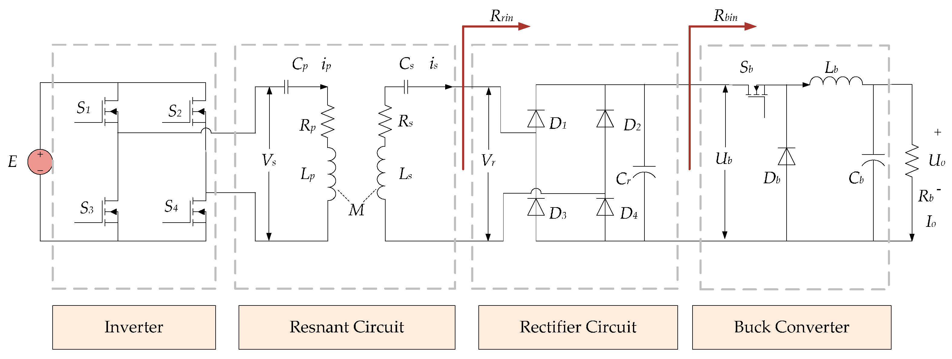
Figure 2.
Continuous current condition waveforms of the system.

Figure 3.
Flowchart of the identification process when considering the two-value issue.

Figure 4.
Primary and secondary series-series (SS) resonant wireless power transfer (WPT) topology.

Figure 5.
Flowchart of the maximum power transfer tracking.

Figure 6.
The control structure of the proposed method.
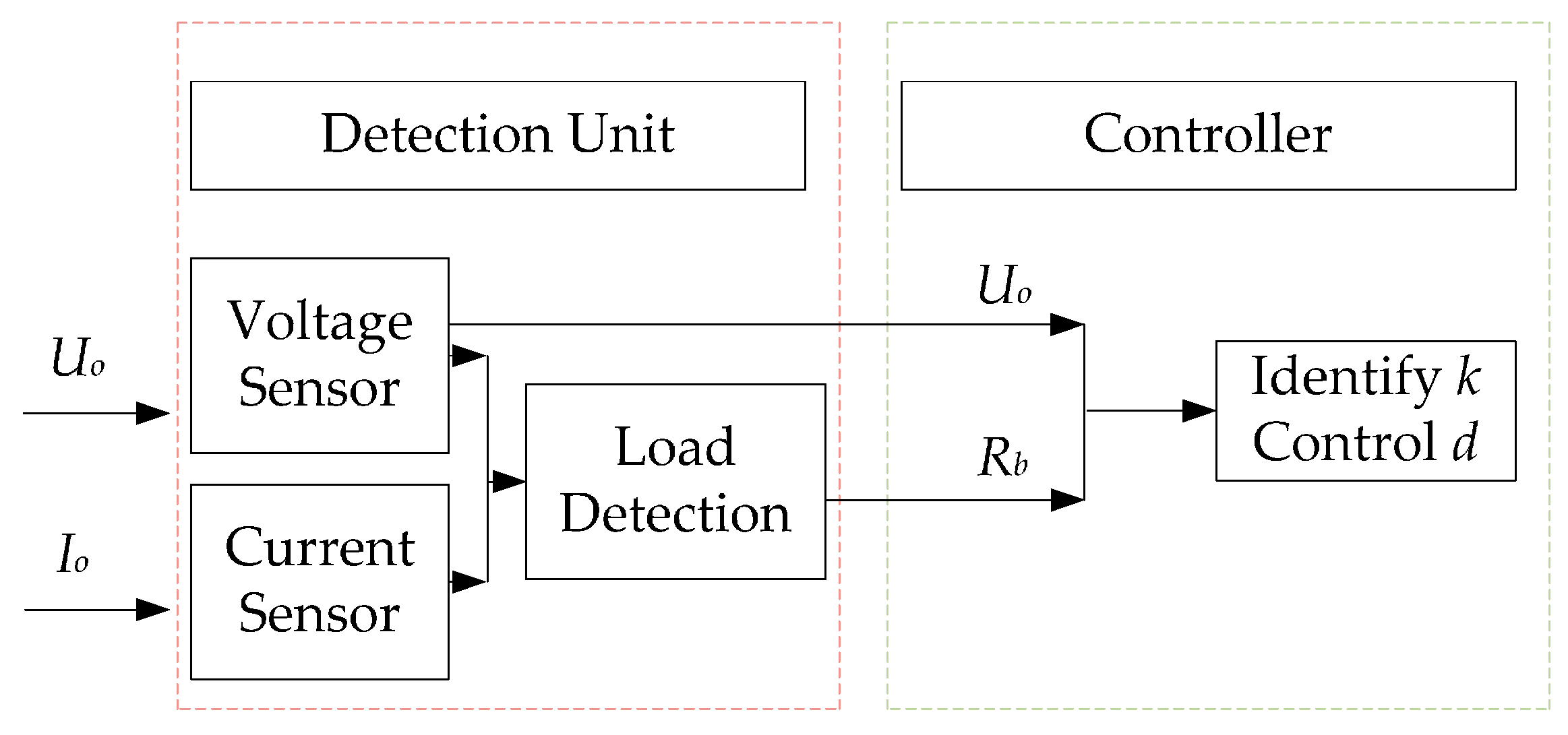
Figure 7.
Identification accuracies of coupling coefficient when d varies from 0.2 to 0.9.

Figure 8.
Maximum power tracking when load Rb changes with different k: (a) k = 0.0811; (b) k = 0.0448.
Figure 8.
Maximum power tracking when load Rb changes with different k: (a) k = 0.0811; (b) k = 0.0448.

Figure 9.
Simulation analysis of system efficiencies under maximum power transfer tracking (MPTT) condition.
Figure 9.
Simulation analysis of system efficiencies under maximum power transfer tracking (MPTT) condition.

Figure 10.
The experimental setup.
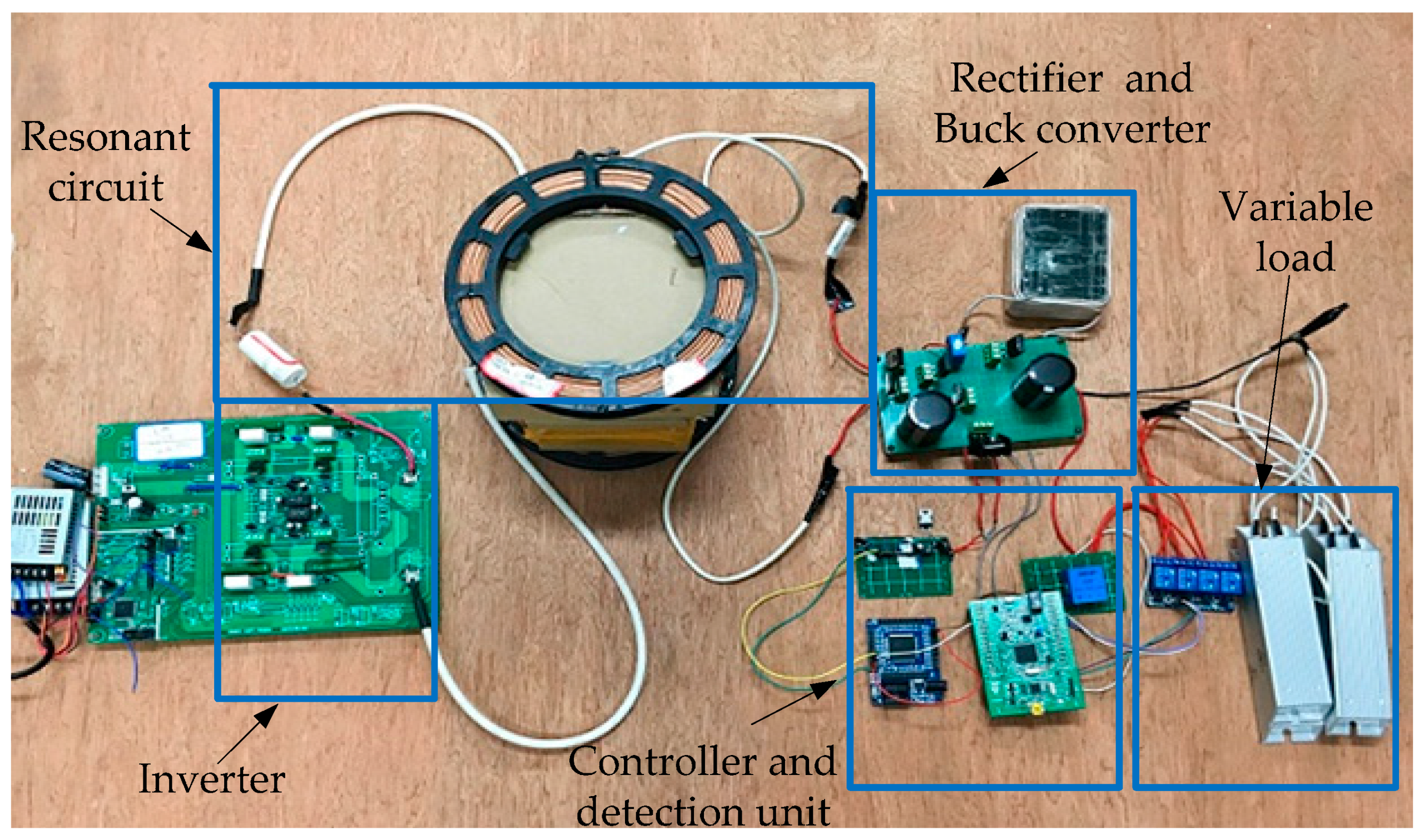
Figure 11.
Experimental MPTT results when load Rb changes with different k: (a) k = 0.0811; (b) k = 0.0448.
Figure 11.
Experimental MPTT results when load Rb changes with different k: (a) k = 0.0811; (b) k = 0.0448.
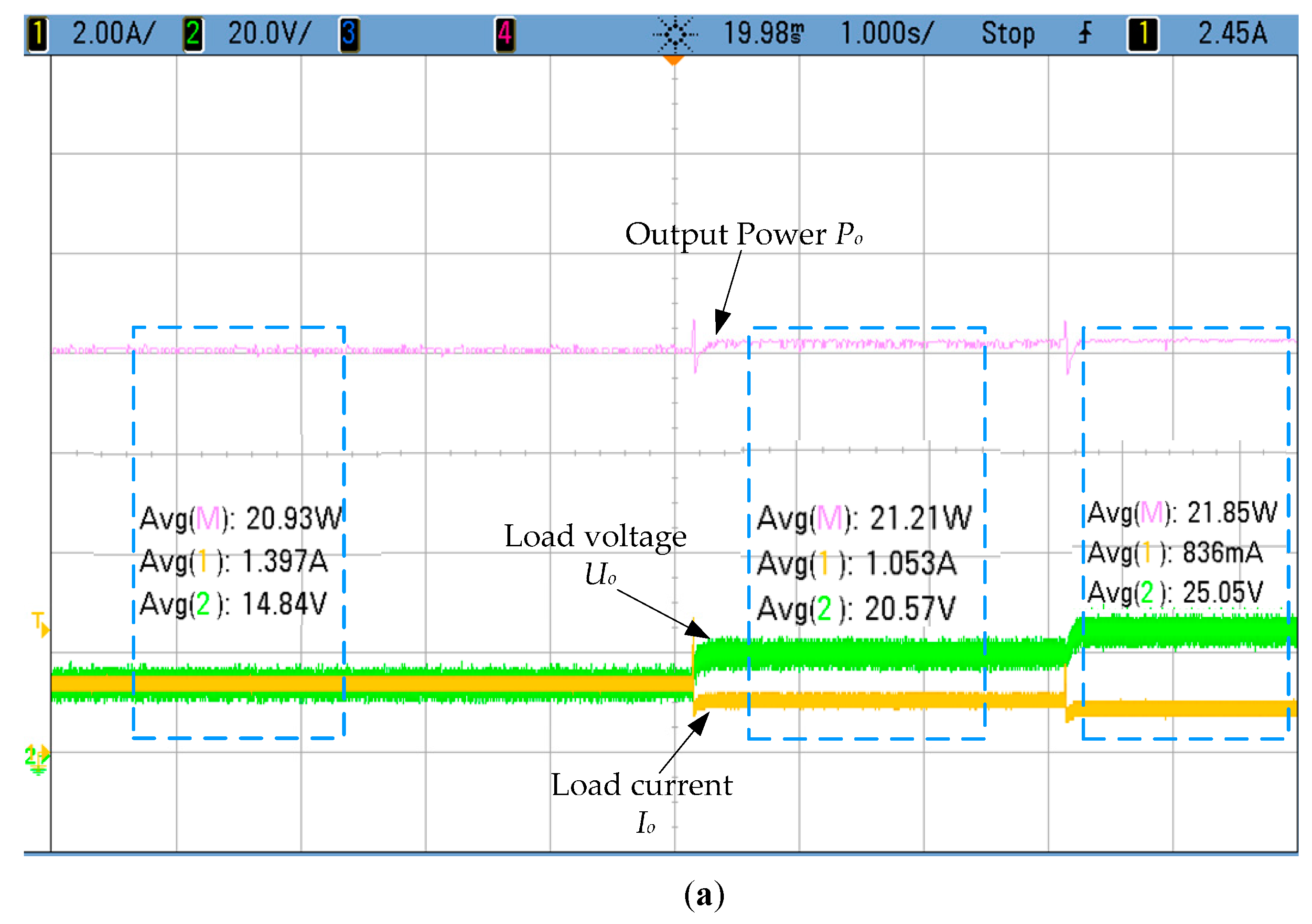

Figure 12.
Experimental analysis of system efficiencies under MPTT condition.


Table 1.
Parameters of the system.
| Items | Parameter | Value | Parameter | Value |
|---|---|---|---|---|
| Resonant circuits | Lp | 365.96 µH | Ls | 363.68 µH |
| Rp | 0.83 Ω | Rs | 0.51 Ω | |
| Cp | 34.25 nF | Cs | 34.30 nF | |
| Litz-wire coils | Diameter | 14 cm | Number of turns | 25 |
| Frequencies | f | 45 kHz | fb | 100 kHz |
| Buck converter | Lb | 120 µH | Cb | 470 µF |
| Input source | E | 10 V |
Table 2.
Coupling coefficient identification with d is 0.5, 0.6 and Rb is 10 Ω.
| Reference k | Identified k | Accuracy |
|---|---|---|
| 0.0448 | 0.0474 | 94.16% |
| 0.0811 | 0.0839 | 96.59% |
| 0.0930 | 0.0962 | 96.67% |
| 0.1500 | 0.1531 | 97.93% |
| 0.2000 | 0.2037 | 98.15% |
| 0.2500 | 0.2546 | 98.16% |
Table 3.
Identification process and results of k.
| Separation Distance | Reference k | Motivating d1 | Motivating d2 | Identified k | Accuracy |
|---|---|---|---|---|---|
| 6 cm | 0.0811 | d1 = 0.5 k1 = 0.0877; k2 = 0.0183 | d2 = 0.6 k3 = 0.0854; k4 = 0.0098 | 0.0866 | 93.2% |
| 9 cm | 0.0448 | d1 = 0.5 k1 = 0.0484; k2 = 0.0332 | d2 = 0.6 k3 = 0.0464; k4 = 0.0207 | 0.0474 | 94.2% |
© 2017 by the authors. Licensee MDPI, Basel, Switzerland. This article is an open access article distributed under the terms and conditions of the Creative Commons Attribution (CC BY) license (http://creativecommons.org/licenses/by/4.0/).
Share and Cite
MDPI and ACS Style
Dai, X.; Li, X.; Li, Y.; Deng, P.; Tang, C. A Maximum Power Transfer Tracking Method for WPT Systems with Coupling Coefficient Identification Considering Two-Value Problem. Energies 2017, 10, 1665. https://doi.org/10.3390/en10101665
AMA Style
Dai X, Li X, Li Y, Deng P, Tang C. A Maximum Power Transfer Tracking Method for WPT Systems with Coupling Coefficient Identification Considering Two-Value Problem. Energies. 2017; 10(10):1665. https://doi.org/10.3390/en10101665
Chicago/Turabian StyleDai, Xin, Xiaofei Li, Yanling Li, Pengqi Deng, and Chunsen Tang. 2017. "A Maximum Power Transfer Tracking Method for WPT Systems with Coupling Coefficient Identification Considering Two-Value Problem" Energies 10, no. 10: 1665. https://doi.org/10.3390/en10101665
Note that from the first issue of 2016, this journal uses article numbers instead of page numbers. See further details here.