Energy Production by Means of Pumps As Turbines in Water Distribution Networks


Dipartimento di Ingegneria, Università degli Studi di Ferrara, 44122 Ferrara, Italy
*
Author to whom correspondence should be addressed.
Energies 2017, 10(10), 1666; https://doi.org/10.3390/en10101666
Submission received: 28 September 2017
/
Revised: 13 October 2017
/
Accepted: 18 October 2017
/
Published: 20 October 2017
Abstract
:This paper deals with the estimation of the energy production by means of pumps used as turbines to exploit residual hydraulic energy, as in the case of available head and flow rate in water distribution networks. To this aim, four pumps with different characteristics are investigated to estimate the producible yearly electric energy. The performance curves of Pumps As Turbines (PATs), which relate head, power, and efficiency to the volume flow rate over the entire PAT operation range, were derived by using published experimental data. The four considered water distribution networks, for which experimental data taken during one year were available, are characterized by significantly different hydraulic features (average flow rate in the range 10–116 L/s; average pressure reduction in the range 12–53 m). Therefore, energy production accounts for actual flow rate and head variability over the year. The conversion efficiency is also estimated, for both the whole water distribution network and the PAT alone.
1. Introduction
To a greater or lesser extent, all of water distribution networks (WDNs) are affected by leakages [1]; these leakages cause economic losses and environmental concerns due to the amount and cost of lost water and energy consumed by pumping stations, which must handle larger volumes of water than those effectively delivered to the users [2]. The rate of water losses in a leaking pipe of a water distribution system is strictly related to the pressure value [1,3]: the higher the pressure, the larger the water volume lost. Therefore, pressure control strategies should be adopted to minimize excessive pressures as far as possible, while ensuring sufficient pressures to satisfy customer demands at all times. As the complexity of a water distribution system grows, the task of achieving the optimal target pressure level becomes more difficult [4].
Operatively, pressure control in WDNs can be achieved by creating district metered areas [5] and/or placing Pressure Reducing Valves (PRVs) [6] to prevent the downstream hydraulic pressure from exceeding the desired value. PRVs are variable closure devices that reduce the conveyance capacity of the pipe by increasing the pressure losses [4]. Therefore, at present, the number of PRVs is increasing in real WDNs and, in the framework of a virtuous energy policy, any attempt should also be made by water network managers to convert energy dissipation into energy production [7].
The theoretical convertible power is considerable and could lead to large energy savings; for instance, according to some recent studies, it may be in the order of 4.7 MW in Germany [7] or about 17 MW in UK water industry [8]. Nevertheless, energy production in water supply systems has only been realized in few cases and mainly in the transmission pipelines, where the available hydraulic power is considerable and fairly constant. Conversely, the dissipation nodes in urban WDNs usually present a large variability in flow rate and head drop, and thus sustainable energy production within WDNs still represents an open challenge.
As highlighted in [9], among the different turbines that can be coupled with low and variable power, Pump As Turbines (PATs) can be considered as a good alternative, since they combine low installation costs with an acceptable energy production. Indeed, pumps can be used in turbine mode by reversing flow direction with the engine acting as a generator [10]. The use of PATs may also increase WDN flexibility, e.g., by changing PAT working conditions in case of pipe failure.
One of the main challenges is that pump manufactures do not usually provide the performance curves of pumps in reverse operation and the designer should face a lack of data that constitutes an obstacle to the choice of the most suitable machine. Therefore, establishing a correlation that enables the transfer from “pump” characteristics into “turbine” characteristics is crucial.
Many researchers have presented some theoretical and empirical relationships for predicting the Best Efficiency Point (BEP) of a PAT [11,12,13,14], while so far a procedure to estimate their performance in turbine mode over the entire operation range is not completely established in literature. In fact, experimental characterization is usually required ad hoc and case by case. Despite the models available in existing literature, predicting PAT curves is still an open issue, because of the lack of information provided by manufacturers and the few laboratory tests that focus on the topic [15]. In [16], a one-dimensional numerical code was presented with the aim of identifying the geometry and performance of a generic PAT on the basis of passage sections and losses in each section of the machine. The paper [17] presented a comprehensive correlation aimed at bringing out the prediction of the turbine mode operation of centrifugal pumps. The authors also developed a physics-based simulation model, aimed at predicting the performance curves of pumps as turbines (PATs) on the basis of the performance curves of the respective pump [18]. The prediction reliability of the simulation model was also compared to that of alternative approaches [19].
In this framework, this paper evaluates the energy potential of four different PATs (characterized by means of experimental performance curves) installed in four different WDNs (also characterized by means of experimental data). The result of the analysis is the estimation of the producible electric energy and the corresponding conversion efficiency from the available hydraulic energy. To overcome the challenge of estimating PAT performance curves, and therefore to improve the reliability of the estimation of the producible electric energy, PAT performance curves over the entire range of operation are taken from published data reported in technical literature. For this reason, the results presented in this paper can be used as a guideline for a preliminary evaluation of energy and economic feasibility of PATs aimed at exploiting the hydraulic energy potential of water distribution networks. This represents the main novel contribution of this paper, as few papers in literature (e.g., [7]) deal with PAT energy potential by considering field data of water distributions networks.
This paper is organized as follows. Pump and PAT performance curves are presented in Section 2; the main characteristics of the real case WDNs are provided in Section 3; the results of the analysis of PATs’ energy potential for the considered case studies are presented and discussed in Section 4; finally, conclusions are provided.
2. Pump and PAT Performance
2.1. Available Field Data from Literature
The starting point for deriving pump and PAT performance curves over the entire range of operation is the paper [11], authored by Derakhshan and Nourbakhsh. The authors reported the performance data taken experimentally on four different turbomachines, running in both pump and PAT mode. The four pumps are characterized by values of the specific speed Ω in the range 1.53–5.82.
The pump characteristic values at the respective BEP are reported in Table 1. These values are calculated in this paper by considering that the experimental non-dimensional data reported in [11] were taken at rotational speed n equal to 25 rps (i.e., 1500 rpm) and pump nominal diameter D was equal to 0.25 m. Moreover, it has to be highlighted that values of specific speed, flow rate, and efficiency were explicitly reported in [11], while head drop is estimated by means of the interpolation curves discussed in Section 2.2, and, accordingly, power is calculated as ρQgH/η.
It can be seen that the four pumps are characterized by considerably different values of power, from about 3 kW to about 22 kW. Accordingly, the volume flow rate at BEP passes from 8.0 L/s to 107.7 L/s and the maximum efficiency increases from 64.5 to 86.8%. Otherwise, the head at BEP decreases from 24.9 m to 18.3 m, passing from pump #1 to pump #4.
Table 2 reports the operating ranges of the four pumps/PATs. It can be seen that the four considered pumps can swallow up to 148 L/s (pump #4), with a maximum head of 29 m (pump #1), maximum power consumption of about 25 kW, and maximum efficiency of 87% (both maximum power and maximum efficiency values refer to pump #4).
Instead, the maximum volume flow rate allowed for PAT operation is slightly lower than that of the pump (i.e., up to 129 L/s for PAT #4). The required head is rather different for the four PATs, e.g., it is in the range 27–68 m for PAT #1 and 12–27 m for PAT #4. The maximum producible electric power passes from less than 5 kW (PAT #1) to more than 25 kW (PAT #4). Moreover, the maximum value of efficiency in PAT mode is lower than the maximum efficiency in pump mode.
2.2. Pump and PAT Performance Curves
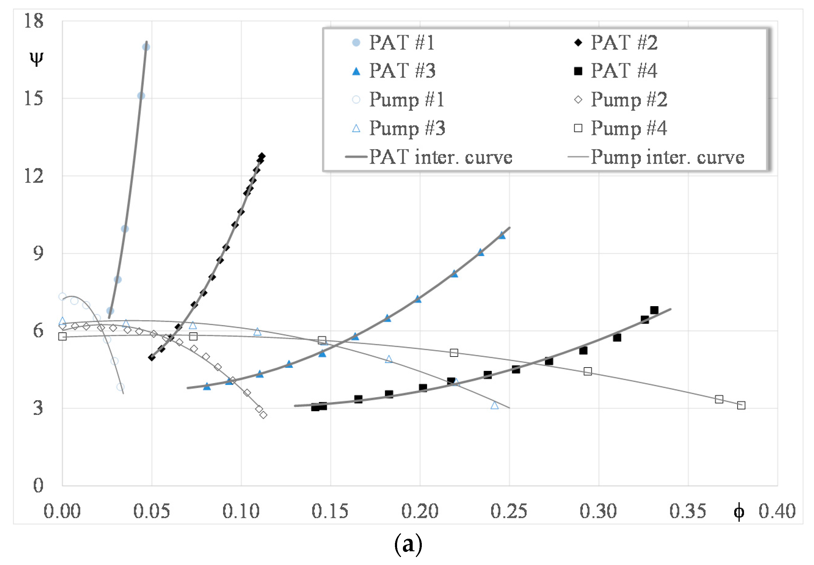
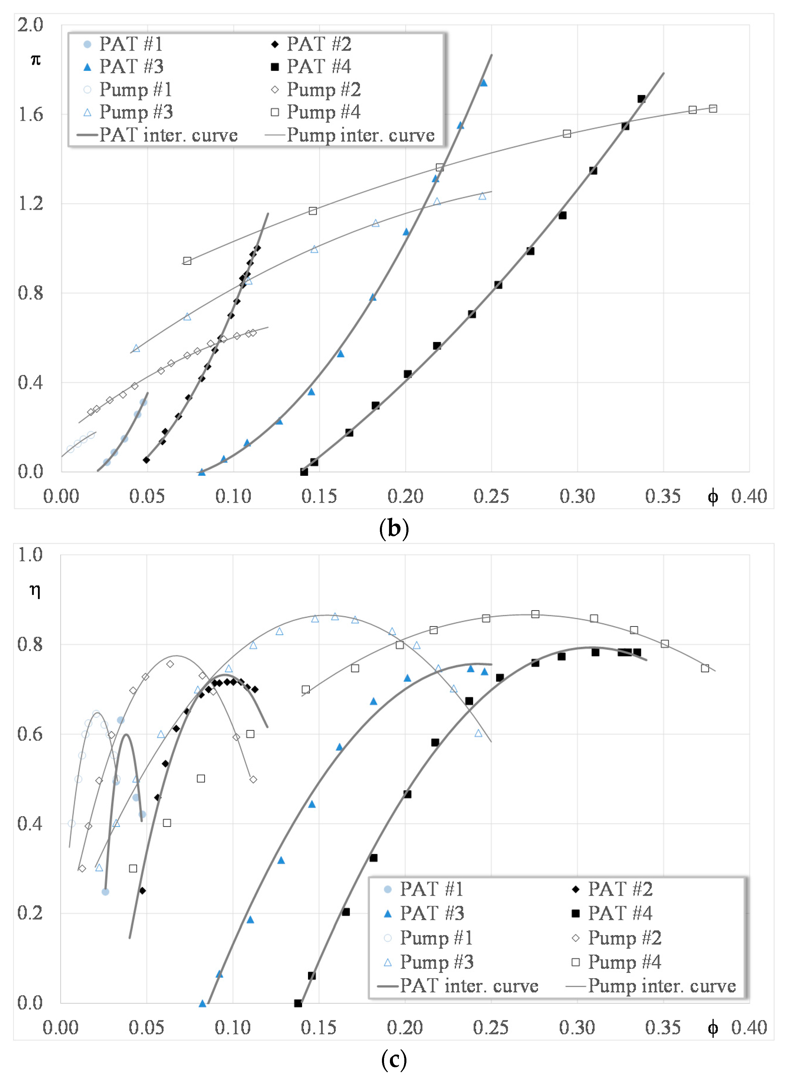
In this paper, pump and PAT behavior was modelled independently, by interpolating the available experimental data reported in [11]. A functional dependence by means of a second-order, third-order, and fourth-order polynomial was investigated for the three non-dimensional performance parameters ψ (non-dimensional head), π (non-dimensional power), and η (efficiency), as a function of the non-dimensional volume flow rate (ϕ). The second-order polynomial functions proved the best fit for all the non-dimensional parameters Y (which plays the role of the three non-dimensional performance parameters ψ, π and η), both for the pump and the PAT, according to Equations (1) and (2), respectively.
Yp(Ω,ϕ) = a2p(Ω)ϕ2 + a1p(Ω)ϕ + a0p(Ω)
YPAT(Ω,ϕ) = a2PAT(Ω)ϕ2 + a1PAT(Ω)ϕ + a0PAT(Ω)
The interpolation curves expressed in Equations (1) and (2) are reported in Figure 1a–c. In these figures, the non-dimensional flow rate is assumed positive, for both the pump and the PAT. As can be seen, this representation also allows for a physically consistent modeling over the entire range of operation. However, it has to be pointed out that these interpolations are valid only in the limited examined range, while they may give rise to incongruences outside the respective range of validity, as can be seen e.g., in Figure 1a for pump #1.
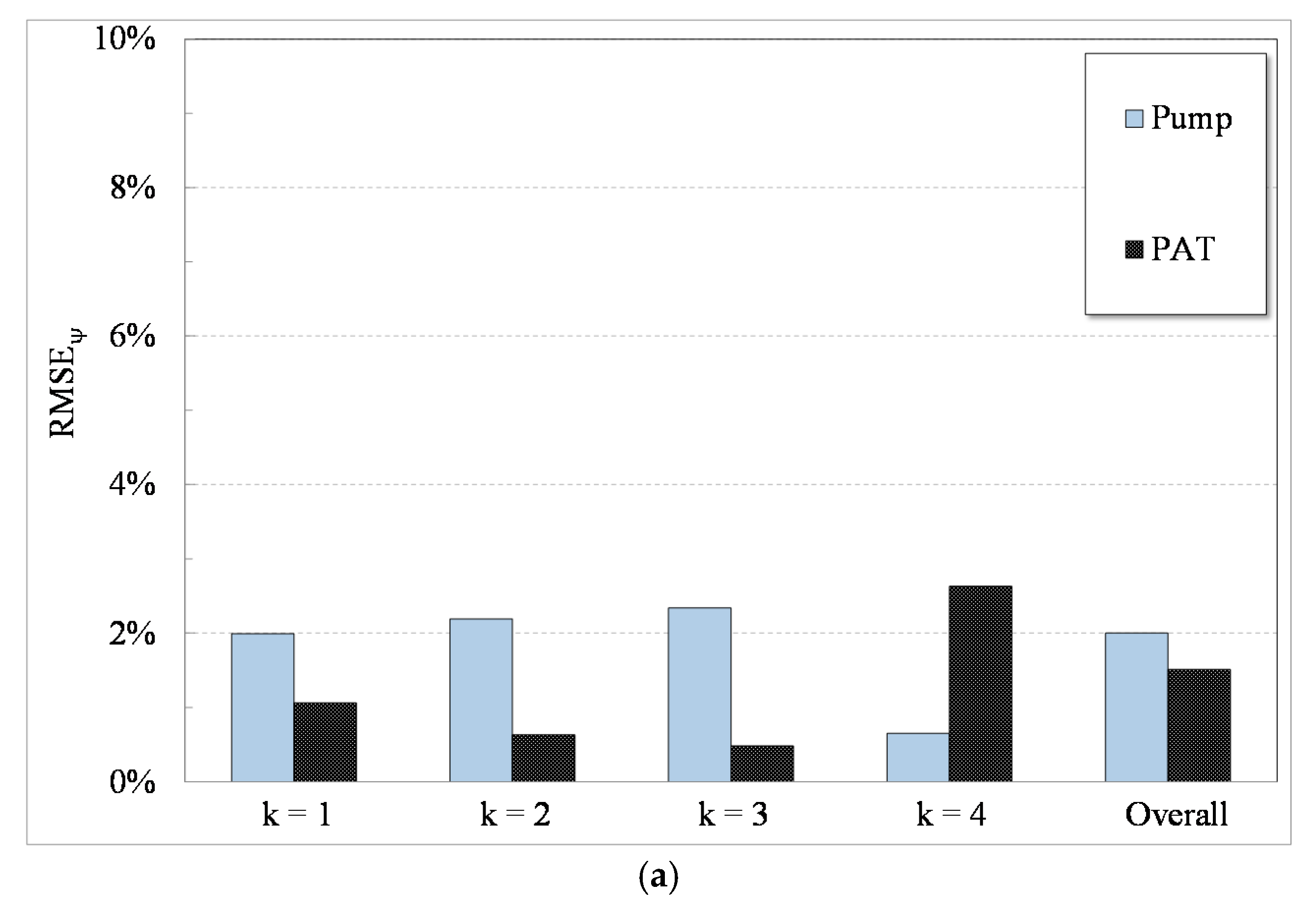
To assess the prediction reliability of the selected modeling approach, the Root Mean Square Error RMSEYk, expressed in Equation (3), is adopted:
The index defined in Equation (3) compares each experimental value of the performance parameter (Yki)e for a given turbomachine k (both in pump and PAT mode) to the corresponding simulated value (Yki)s, predicted by means of Equations (1) and (2).
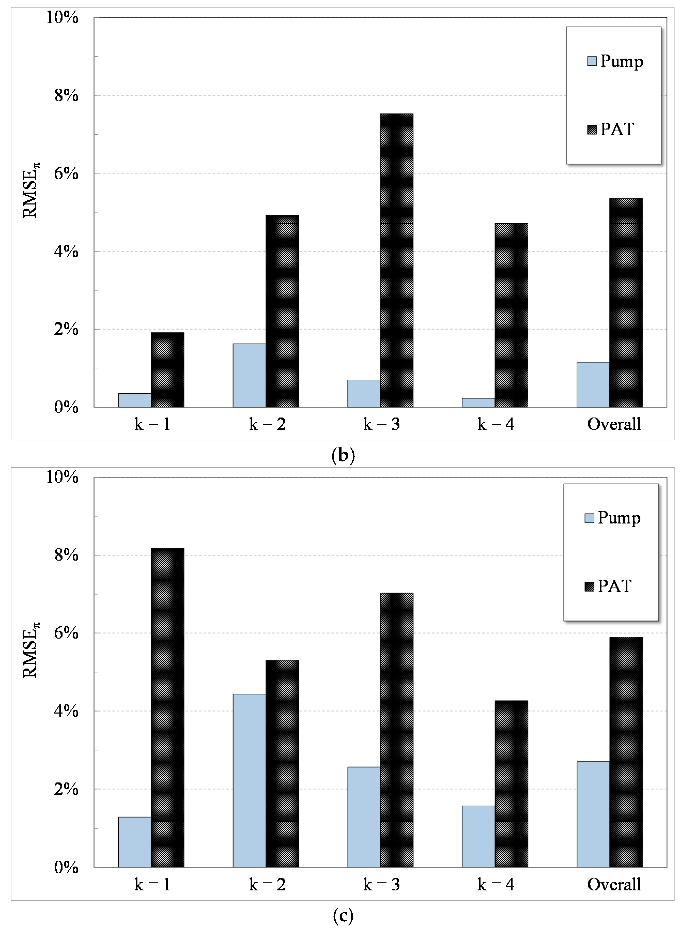
The values of RMSEYk are summarized in Figure 2. It can be noticed that, in general, RMSEψ values are very good in both pump and PAT mode (they are in the range 0.5–2.6%). Moreover, RMSEπ values in pump mode are even better (values in the range 0.2–1.6%). Otherwise, RMSEπ values in PAT mode are considerably higher (values in the range 1.9–7.5%), and this also reflects on the values of RMSEη. However, the selected interpolating functions expressed in Equations (1) and (2) are considered satisfactory for the purpose of this paper, since they provide a physics-responding approach for simulating the behavior of pumps and PATs over the entire range of operation.
3. Field Data of Water Distribution Networks
3.1. Water Distribution Networks
The four water distribution networks (WDN A, B, C, and D) considered in this paper are located in Italy. WDN A and WDN B serve two small towns, featuring around 950 and 2100 users, respectively. WDN C serves a part of a large city, featuring around 8500 users, while WDN D serves a district featuring around 5000 users. The total length of each system is about 45 km, 102 km, 150 km, and 120 km for WDN A, B, C and D, respectively.
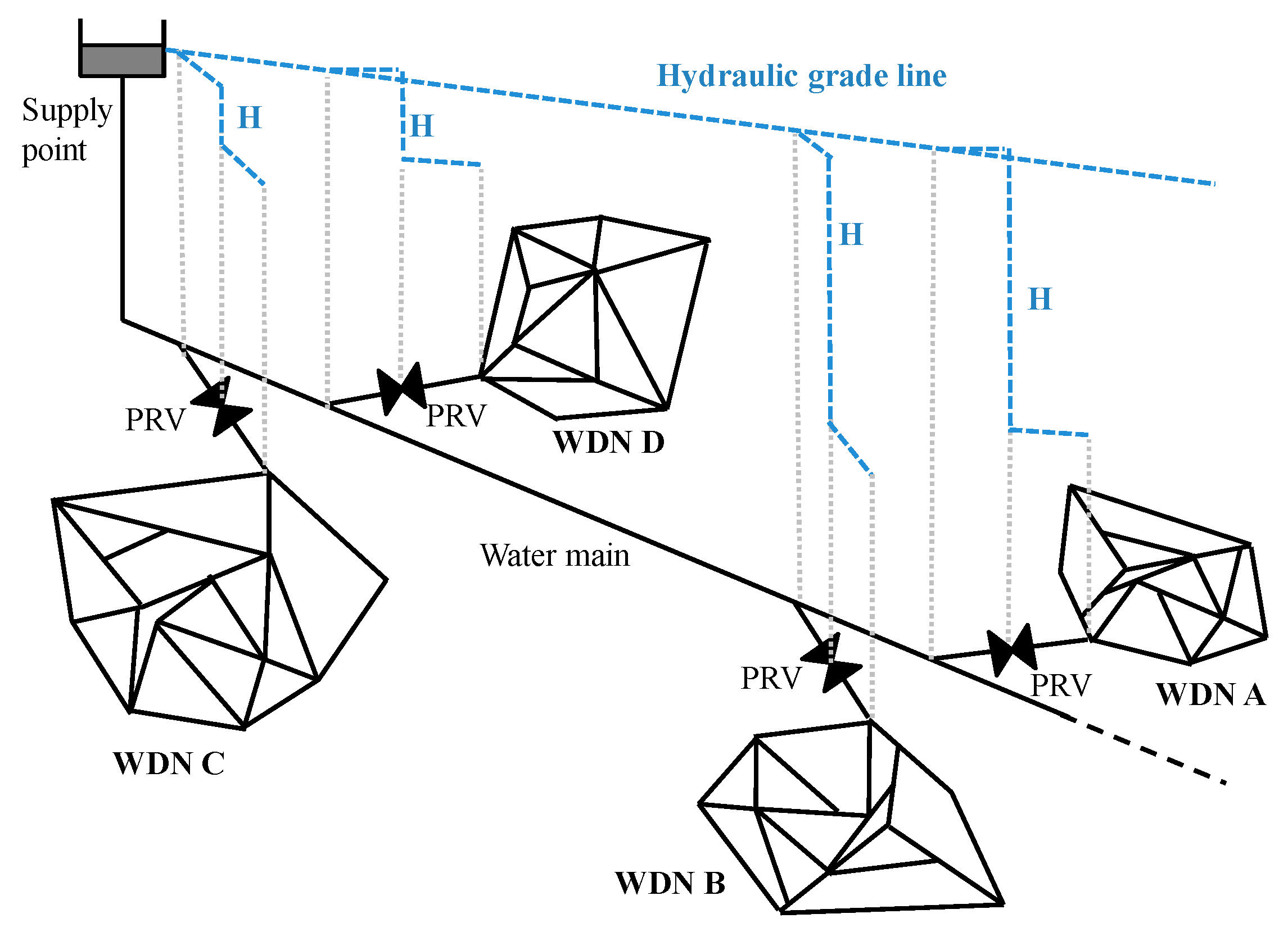
The four WDNs lay at the foot of a hill zone and are fed by the same water supply system, as shown in Figure 3. In particular, each WDN is connected to the water main in just one point; a PRV is currently located at each connection point in order to reduce the downstream pressure since the pressure within the water main is considerably higher than that required within the distribution system. Indeed, within each WDN, the pressure is fixed at around 35 m, while the pressure within the main varies from around 80 m to 90 m (next to WDN A and B, which are located in the lowest part of the served area) to around 45 m (next to WDN C and WDN D, which are located in the highest part of the served area). Consequently, the head drop is considerably larger at the PRVs located at the inlet point of WDN A and B, whereas it is lower at the PRV located at the inlet point of WDN C and D.
As discussed in the Introduction, such a layout allows an effective pressure control within the network, leading to significant benefits in terms of leakage reduction. On the other hand, a significant amount of energy is currently wasted in correspondence of each PRV.
3.2. WDN Field Data
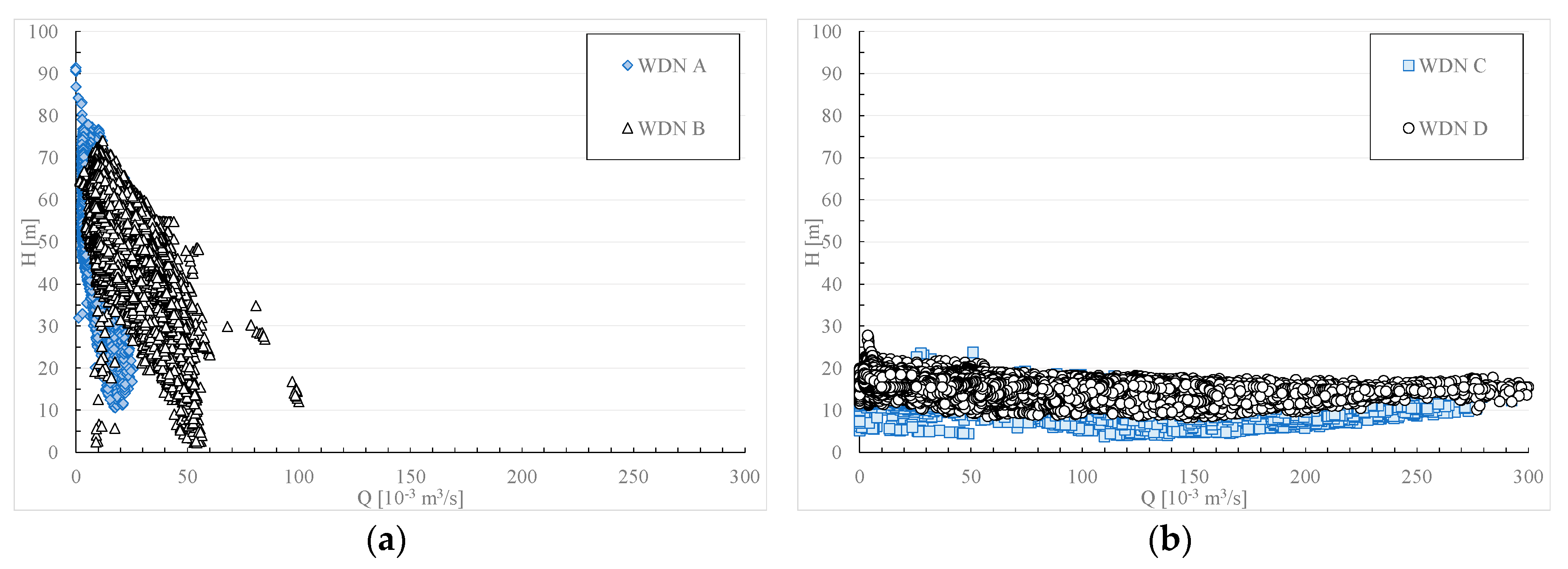
The available field data were taken over one year (year 2013), every 15 min. Therefore, 35,040 measured data sets are available per each WDN. Each data set consists of two measured parameters: the volume flow rate Q and the head drop H. All of the available field data are shown in Figure 4, while Figure 5 reports the main characteristics of the four WDNs.
According to Figure 4, WDN A and B are characterized by similar values of head drop at the inlet point (roughly in the range 20–80 m), while WDN C and WDN D have a significantly lower average head drop at the inlet point (roughly in the range 5–25 m). Instead, according to Figure 5, the average volume flow rate changes dramatically from WDN A (10 L/s) to WDN C (116 L/s), while it is 28 L/s for WDN B. Moreover, several peak values of head drop were measured in WDN A (up to about 90 m) in correspondence of the smallest values of the volume flow rate. Otherwise, WDN C and WDN D are characterized by almost regular values of head drop (average value equal to 12 m), but the volume flow rate is usually considerably higher than that of WDN A and B (mean value: 116 L/s; maximum value: 292 L/s). Finally, it has to be observed that WDN D has an average head drop similar to that of WDN C (16 m), but the average flow rate is significantly lower (49 L/s). Therefore, the four WDNs are representative of different scenarios, which challenge the installation of a PAT to a different extent.
4. Results
The aim of the analysis reported in this section is twofold:
- (1)
- Assessment of the energy potential of otherwise-wasted hydraulic energy. The yearly producible electric energy is obtained by considering the actual PAT working point for each data set. The working point is set by acting on two valves, as outlined in Section 4.1;
- (2)
- Estimation of the conversion efficiency of energy recovery, for both the entire WDN (overall efficiency) and for the PAT alone (PAT efficiency).
4.1. Producible Energy
The procedure adopted to evaluate the energy production by means of a PAT consists of the steps reported below:
- (1)
- availability of pump performance curves over the entire range of operation. In this paper, four pumps (#1 through #4) are evaluated;
- (2)
- estimation of PAT’s performance curves over the entire range of operation, as described in Section 2.2;
- (3)
- estimation of the producible electric power for each data set (i.e., for each time point), by considering that:
- If HPAT ≤ Hmeas, the producible electric power is calculated at Qmeas and HPAT. This means that there is a reduction of H, so that ΔHun = Hmeas − HPAT is unexploited. In other words, available head has to be dissipated;
- If HPAT > Hmeas, the producible electric power is calculated at Qthr (lower than Qmeas) and Hmeas. In fact, the volume flow rate flowing through the PAT has to be decreased, so that, in this case, ΔQun = Qmeas − Qthr is unexploited;
- (4)
- calculation of the producible electric energy by multiplying the producible electric power by the sampling time of WDN data (in this paper, 15 min); and,
- (5)
- calculation of the producible electric energy over one year.
As it can be observed, the regulation system is assumed in this paper as simple as possible to lower both installation and operation costs. In fact, it is composed of only two valves: one valve in series with the PAT, to dissipate the excess pressure/head, and one valve in parallel (bypass valve), which can be opened to reduce the volume flow rate through the PAT to the value that makes HPAT equal to Hmeas. This regulation strategy was also discussed and investigated in [20] (where it was identified as “hydraulic regulation”) and represents a feasible operation mode for WDNs. It is clear that the possibility of varying PAT’s rotational speed and consequently moving PAT’s characteristic curve in order to match, at each time point, the available head and flow rate, may increase the producible electric energy, but would require the use of an inverter and a more sophisticated regulation system.
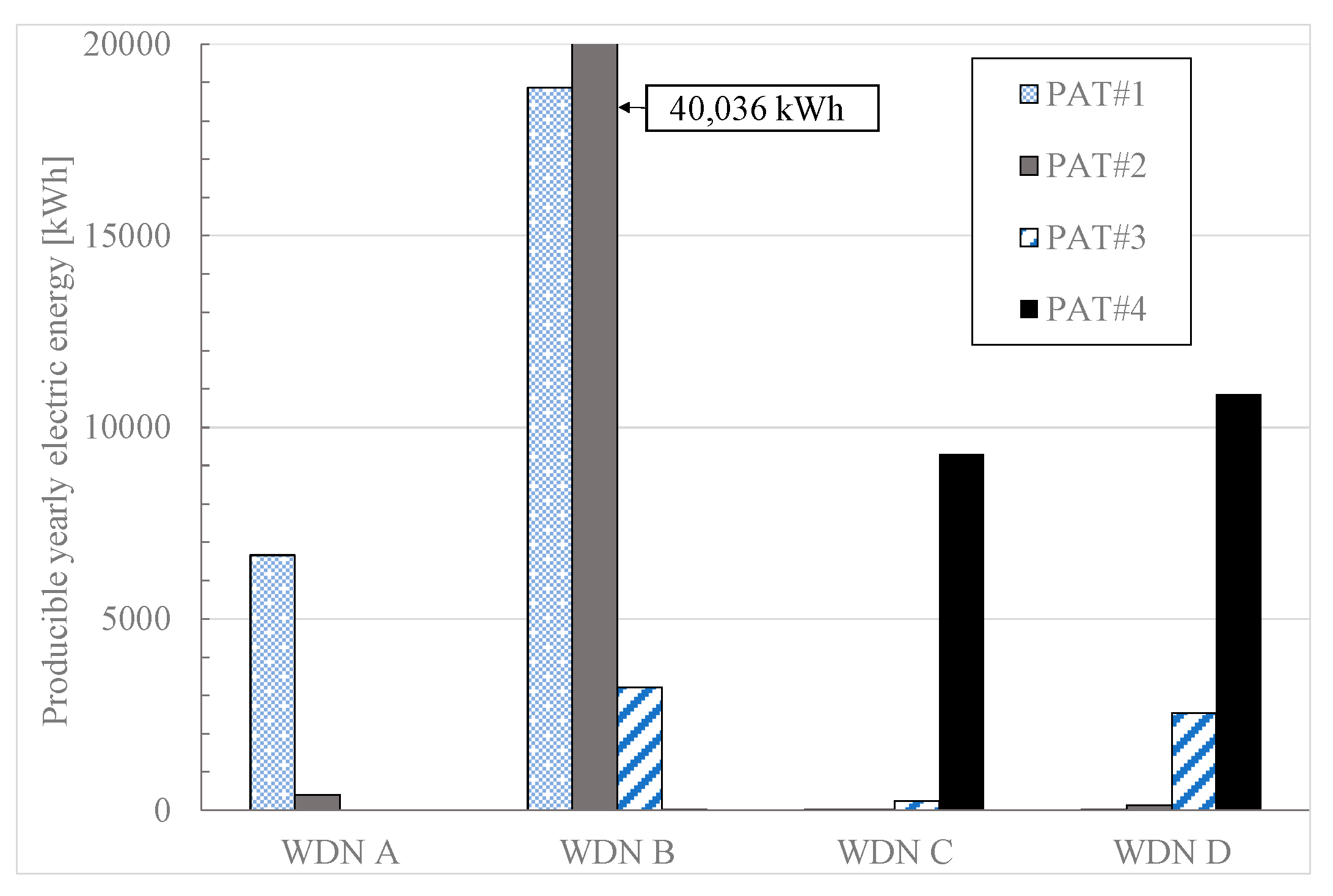
The producible yearly electric energy, estimated according to the procedure outlined above, is reported in Figure 6. It can be seen that, for all the four WDNs, an optimal solution which is by far preferable with respect to other possible combinations can be identified, i.e., PAT #1 for WDN A, PAT #2 for WDN B and PAT #4 for both WDN C and WDN D. This is clearly due to the matching of PAT’s performance curves (see Figure 1) and WDN characteristics (see Figure 4 and Figure 5). The value of the maximum producible yearly electric energy is almost comparable for WDN A, WDN C, and WDN D (6650 kWh, 9293 kWh and 10,867 kWh, respectively), while it is considerably higher for WDN B (40,036 kWh). In fact, on average, the WDN B is characterized by a combination of higher flow rate and head (see Figure 4). However, it can be noted that, in all of the combinations, the producible yearly electric energy is rather low. For instance, the producible yearly electric energy can be compared to the residential electricity consumption per capita in 2010 in the EU-27, which was equal to 1682 kWh [21]. Thus, in the best case, the electric energy demand of only twenty-four household users can be met.
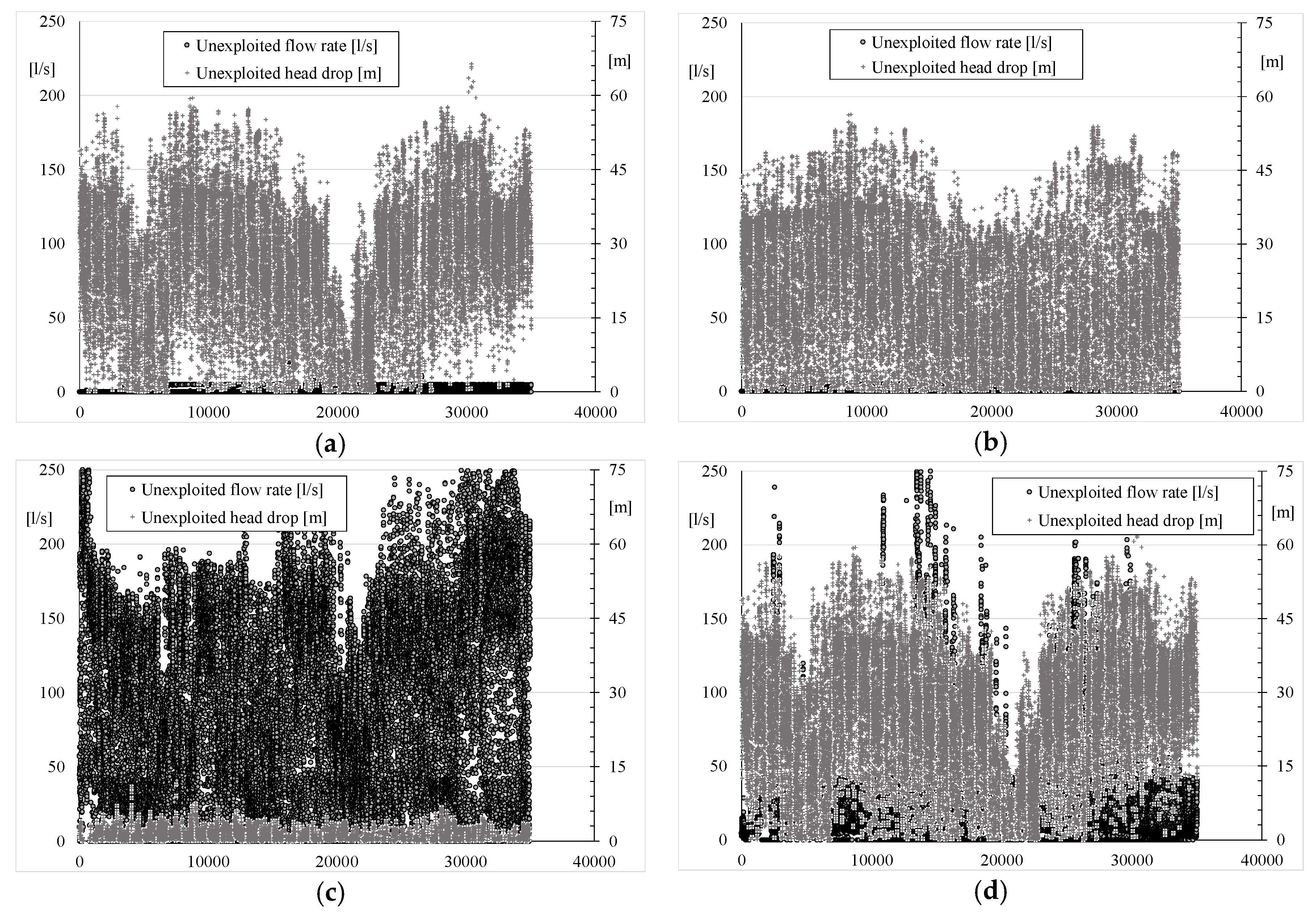
The energy potential which cannot be exploited is reported in Figure 8, only for the four best combinations of WDN/PAT. It can be seen that the two solutions WDN A/PAT #1 and WDN B/PAT #2 are similar, i.e., available head is usually wasted. Otherwise, for the solution WDN C/PAT #4, a considerable amount of volume flow rate is always unexploited (at least 100 L/s). Instead, the solution WDN D/PAT #4 represents an intermediate case, since both flow rate and head drop are partially wasted. These results are coherent with the analyzed PATs (which may be not the best fit for the considered WDNs) the considered installation scheme and regulation system, which makes use of two valves dissipating excessive pressure and flow rate at fixed rotational speed. Indeed, larger amount of available head and volume flow rate could be exploited by considering an electrical regulation of the rotational speed, even though recent studies pointed out that the latter approach is, on the whole, less efficient and convenient than the former [22].
4.2. Conversion Efficiency
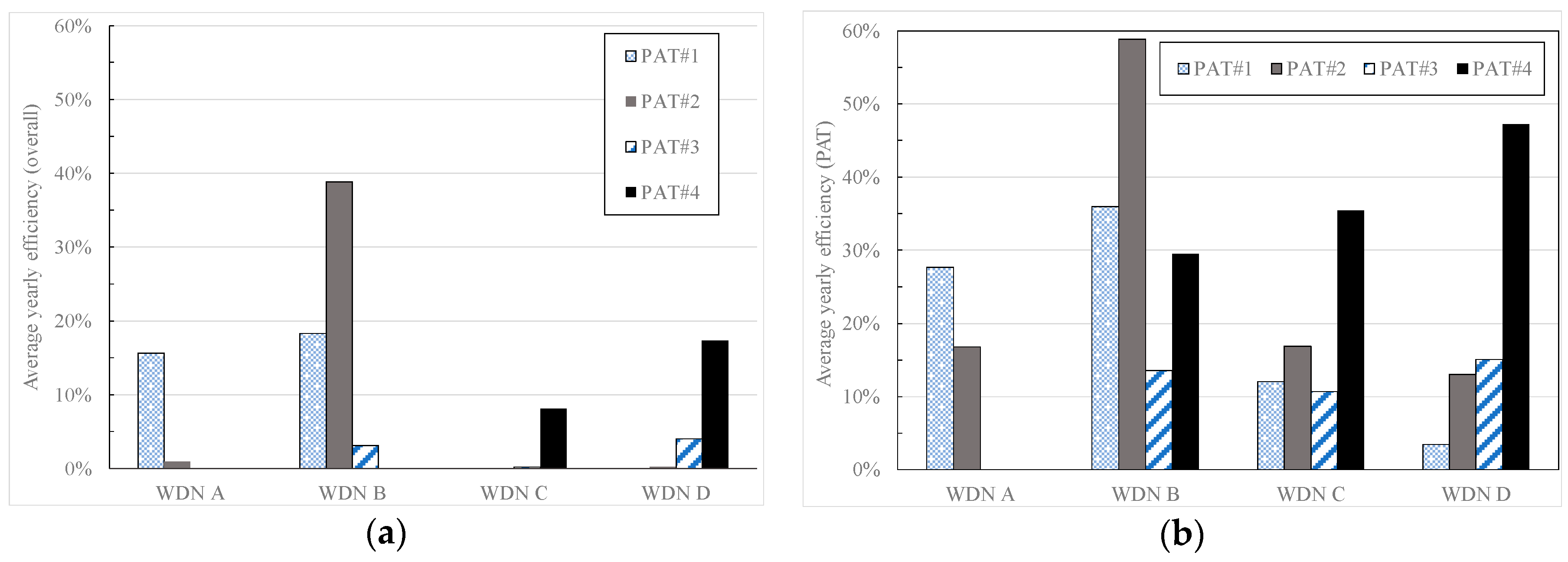
The estimation of the conversion efficiency is carried out by considering both the energy potential from the whole WDN (i.e., available flow rate and head) and PAT internal efficiency. In fact, the former conversion efficiency (overall efficiency) accounts for the incomplete exploitation of flow rate and head observed in Figure 7, while the latter (PAT efficiency) accounts for the fact that the producible electric energy was calculated by considering the actual operating point per each data set (i.e., per each available time point), which, in general, can be considerably far from the BEP.
The results of this analysis are summarized in Figure 8. From an overall perspective (see Figure 8 on the left), the WDN potential is usually rather unexploited, with the exception of one case (WDN B and PAT #2) that has an overall conversion efficiency of 39%. This result is in agreement with a similar analysis carried out in [20] by considering several WDNs: in fact, it was found out, in [20] that only in few cases, the overall efficiency was higher than 40%, while in other few cases it was only about 10%. This obviously demonstrates that the pump to be used as a PAT has to be carefully selected according to the considered WDN. On the other hand, the PAT itself usually runs with an “acceptable” efficiency (see Figure 8 on the right), if it is considered that this type of machine is not designed to work as an expander. The best case is given once again by the PAT #2 installed in the WDN B, which has a yearly average efficiency of 59%.
Another relevant achievement of this analysis is that the estimation of the producible yearly electric energy cannot be made by using all-inclusive values of overall/PAT efficiency. In fact, the PAT actual working point is usually considerably far from BEP (see values in Table 2), and therefore, the estimate carried out by considering BEP values would result considerably overestimated. Instead, the values provided in Figure 8, though valid only for the considered WDNs, can be used as an indication for evaluating PAT energy and economic actual potential.
5. Conclusions
This paper presented an energy analysis aimed at estimating the energy potential of pumps used as turbines (PATs) in order to exploit the available hydraulic energy of water distribution networks. Four pumps, of which the performance both as a pump and as a turbine was known from published experimental data, were tested in four water distribution networks (WDNs), of which the experimental data over one year were also available. The pumps and the WDNs were considerably different, so that the resulting matching could be considered representative of very different scenarios.
By considering the actual variability of flow rate and available head over one year, four optimal matching pump/WDN were identified and the consequent producible electric energy was estimated. The average conversion efficiency was also estimated, for both the overall system and the PAT. It was found out, that from an overall perspective, the WDN potential is usually rather unexploited, with the exception of one case that had a conversion efficiency of 39%.
On the one hand, the analyses carried out in this paper demonstrate that the pump to be used as a PAT has to be carefully selected according to the considered WDN; on the other hand, a considerable amount of head drop and/or flow rate has to be wasted because of the highly variable flow rate and head drop typically be observed in real water distribution systems. In fact, the PAT itself usually runs at “acceptable” efficiency values (up to 59%).
For these reasons, future works will analyze the performance of different PATs coupled with different installation and regulation schemes, in order to maximize the producible electric energy.
Author Contributions
Mauro Venturini, Stefano Alvisi and Silvio Simani conceived and designed the experiments; Mauro Venturini, Stefano Alvisi, Silvio Simani and Lucrezia Manservigi performed the experiments; Mauro Venturini, Stefano Alvisi, Silvio Simani and Lucrezia Manservigi analyzed the data; Mauro Venturini, Stefano Alvisi and Silvio Simani wrote the paper.
Conflicts of Interest
The authors declare no conflict of interest.
Abbreviations
| a | performance curve coefficient |
| D | pump nominal diameter, m |
| g | gravitational acceleration, m/s2 |
| H | head drop, m |
| k | label of pump/PAT |
| n | rotational speed, rps |
| N | number of pump/PAT experimental data |
| P | power, W |
| PAT | Pump As Turbine |
| PRV | Pressure Reducing Valve |
| Q | volume flow rate, m3/s |
| RMSE | root mean square error |
| WDN | water distribution network |
| Y | non-dimensional performance parameter (ψ, π, η) |
| η | efficiency |
| ϕ | non-dimensional volume flow rate defined as Q/(nD3) |
| π | non-dimensional power defined as P/(ρn3D5) |
| ρ | density, kg/m3 |
| ψ | non-dimensional head defined as gH/(n2D2) |
| ω | angular velocity, rad/s |
| Ω | specific speed defined as ωQ0.5/(gH)0.75 |
| Subscripts and superscripts | |
| 1,2,3,4 | label of pump/PAT |
| av | average |
| BEP | best efficiency point |
| e | experimental |
| meas | measured |
| p | pump |
| PAT | pump as turbine |
| s | simulated |
| thr | throttle |
| un | unexploited |
| Y | non-dimensional parameter |
References
- Alvisi, S.; Franchini, M. Multiobjective optimization of rehabilitation and leakage detection scheduling in water distribution systems. Water Resour. Plan. Manag. 2009, 135, 426–439. [Google Scholar] [CrossRef]
- Colombo, A.F.; Karney, B.W. Energy and Costs of Leaky Pipes: Toward Comprehensive Picture. Water Resour. Plan. Manag. 2002, 128, 441–450. [Google Scholar] [CrossRef]
- Araujo, L.; Ramos, H.; Coelho, S. Pressure control for leakage minimisation in water distribution systems management. Water Resour. Manag. 2006, 20, 133–149. [Google Scholar] [CrossRef]
- Giugni, M.; Fontana, N.; Portolano, D. Energy saving policy in water distribution networks. In Proceedings of the International Conference on Renewable Energies and Power Quality (ICREPQ’09), Valencia, Spain, 15–17 April 2009. [Google Scholar]
- Alvisi, S. A New Procedure for Optimal Design of District Metered Areas Based on the Multilevel Balancing and Refinement Algorithm. Water Resour. Manag. 2015, 29, 4397–4409. [Google Scholar] [CrossRef]
- Walsky, T.; Bezts, W.; Posluzny, E.; Weir, M.; Withman, B. Modeling leakage reduction through pressure control. Am. Water Works Assoc. 2006, 98, 148–155. [Google Scholar]
- Carravetta, A.; Del Giudice, G.; Fecarotta, O.; Ramos, H. Energy Production in Water Distribution Networks: A PAT Design Strategy. Water Resour. Manag. 2012, 26, 3947–3959. [Google Scholar] [CrossRef]
- Zakkour, P.; Gochin, R.; Lester, J. Developing a sustainable energy strategy for a water utility. Part II: A review of potential technologies and approaches. Environ. Manag. 2002, 66, 115–125. [Google Scholar] [CrossRef]
- Sammartano, V.; Arico, C.; Carravetta, A.; Fecarotta, O.; Tucciarelli, T. Banki-michell optimal design by computational fluid dynamics testing and hydrodynamic analysis. Energies 2013, 6, 2362–2385. [Google Scholar] [CrossRef] [Green Version]
- Ramos, H.; Borga, A. Pump as turbine: An unconventional solution to energy production. Urban Water 1999, 1, 261–263. [Google Scholar] [CrossRef]
- Derakhshan, S.; Nourbakhsh, A. Experimental Study of Characteristic Curves of Centrifugal Pumps Working as Turbines in Different Specific Speeds. Exp. Therm. Fluid Sci. 2008, 32, 800–807. [Google Scholar] [CrossRef]
- Derakhshan, S.; Nourbakhsh, A. Theoretical, Numerical and Experimental Investigation of Centrifugal Pumps in Reverse Operation. Exp. Therm. Fluid Sci. 2008, 32, 1620–1627. [Google Scholar] [CrossRef]
- Yang, S.; Derakhshan, S.; Kong, F. Theoretical, Numerical and Experimental Prediction of Pump as Turbine Performance. Renew. Energy 2012, 48, 507–513. [Google Scholar] [CrossRef]
- Derakhshan, S.; Kasaeian, N. Optimization, Numerical, and Experimental Study of a Propeller Pump as Turbine. Energy Resour. Technol. 2014, 136, 012005. [Google Scholar] [CrossRef]
- Pugliese, F.; De Paola, F.; Fontana, N.; Giugni, M.; Marini, G. Experimental characterization of two Pumps as Turbines for hydropower generation. Renew. Energy 2016, 99, 180–187. [Google Scholar] [CrossRef]
- Barbarelli, S.; Amelio, M.; Florio, G. Predictive model estimating the performances of centrifugal pumps used as turbines. Energy 2016, 107, 103–121. [Google Scholar] [CrossRef]
- Tan, X.; Engeda, A. Performance of centrifugal pumps running in reverse as turbine: Part II—Systematic specific speed and specific diameter based performance prediction. Renew. Energy 2016, 99, 188–197. [Google Scholar] [CrossRef]
- Venturini, M.; Alvisi, S.; Simani, S.; Manservigi, L. Development of a Physics-Based Model to Predict the Performance of Pumps as Turbines (PATs). In Proceedings of the ECOS 2017, San Diego, CA, USA, 2–6 July 2017. Paper #17. [Google Scholar]
- Venturini, M.; Alvisi, S.; Simani, S.; Manservigi, L. Comparison of Different Approaches to Predict the Performance of Pumps as Turbines (PATs). In Proceedings of the ECOS 2017, San Diego, CA, USA, 2–6 July 2017. Paper #18. [Google Scholar]
- Fecarotta, O.; Aricò, C.; Carravetta, A.; Martino, R.; Ramos, H.M. Hydropower Potential in Water Distribution Networks: Pressure Control by PATs. Water Resour. Manag. 2015, 29, 699–714. [Google Scholar] [CrossRef] [Green Version]
- Bertoldi, P.; Hirl, B.; Labanca, N. Energy Efficiency Status Report 2012; Joint Research Centre JRC 69638; The Publications Office of the European Union: Luxembourg, 2012. [Google Scholar] [CrossRef]
- Carravetta, A.; Del Giudice, G.; Fecarotta, O.; Ramos, H. PAT design strategy for energy recovery in water distribution networks by electrical regulation. Energies 2013, 6, 411–424. [Google Scholar] [CrossRef]
Figure 1.
(a) Non-dimensional head vs. non-dimensional volume flow rate; (b) Non-dimensional power vs. non-dimensional volume flow rate; and, (c) Efficiency vs. non-dimensional volume flow rate (symbols: experimental data reported in [11]; lines: interpolation curves).
Figure 1.
(a) Non-dimensional head vs. non-dimensional volume flow rate; (b) Non-dimensional power vs. non-dimensional volume flow rate; and, (c) Efficiency vs. non-dimensional volume flow rate (symbols: experimental data reported in [11]; lines: interpolation curves).


Figure 2.
RMSEYk values for (a) non-dimensional head; (b) non-dimensional power and (c) efficiency.


Figure 3.
Layout of the four water distribution networks (WDNs).

Figure 4.
Available head drop vs. volume flow rate (measured values). (a) WDN A and B; (b) WDN C and D.
Figure 4.
Available head drop vs. volume flow rate (measured values). (a) WDN A and B; (b) WDN C and D.

Figure 5.
Summary of (a) volume flow rate and (b) head drop for WDN A, B, C and D.

Figure 6.
Producible yearly electric energy.

Figure 7.
Unexploited flow rate and head drop for (a) WDN A and PAT #1; (b) WDN B and PAT #2; (c) WDN C and PAT #4 and (d) WDN D and PAT #4.
Figure 7.
Unexploited flow rate and head drop for (a) WDN A and PAT #1; (b) WDN B and PAT #2; (c) WDN C and PAT #4 and (d) WDN D and PAT #4.

Figure 8.
Average yearly conversion efficiency: (a) overall and (b) PAT.


Table 1.
Pump characteristics at Best Efficiency Point (BEP) [11].
Table 1.
Pump characteristics at Best Efficiency Point (BEP) [11].
| Pump | Ω | Q, (10−3 m3/s) | η, (%) | H, (m) | P, (W) |
|---|---|---|---|---|---|
| #1 | 1.53 | 8.0 | 64.5 | 24.9 | 3044 |
| #2 | 2.41 | 24.8 | 75.7 | 22.1 | 7114 |
| #3 | 3.94 | 62.2 | 86.3 | 21.1 | 14,926 |
| #4 | 5.82 | 107.7 | 86.8 | 18.3 | 22,288 |
Table 2.
Pump and pumps used as turbines (PAT) operating range reported in [11].
Table 2.
Pump and pumps used as turbines (PAT) operating range reported in [11].
| Pump | Q, (10−3 m3/s) | H, (m) | P, (W) | η, (%) |
| #1 | 0.0–12.7 | 15.3–29.2 | 1559–2525 | 40.1–64.5 |
| #2 | 0.0–43.9 | 10.9–24.7 | 4084–9504 | 30.0–75.7 |
| #3 | 0.0–94.4 | 12.5–25.5 | 8465–18,860 | 30.3–86.3 |
| #4 | 0.0–148.3 | 12.4–23.1 | 14,405–24,800 | 30.0–86.8 |
| PAT | Q, (10−3 m3/s) | H, (m) | P, (W) | η, (%) |
| #1 | 10.4–18.3 | 27.0–67.7 | 668–4752 | 24.8–63.1 |
| #2 | 19.5–43.5 | 19.8–50.8 | 817–15,296 | 25.1–71.6 |
| #3 | 31.5–95.9 | 15.4–38.7 | 0–26,582 | 0.0–74.7 |
| #4 | 55.2–129.3 | 12.1–27.1 | 0–25,468 | 0.0–78.3 |
© 2017 by the authors. Licensee MDPI, Basel, Switzerland. This article is an open access article distributed under the terms and conditions of the Creative Commons Attribution (CC BY) license (http://creativecommons.org/licenses/by/4.0/).
Share and Cite
MDPI and ACS Style
Venturini, M.; Alvisi, S.; Simani, S.; Manservigi, L. Energy Production by Means of Pumps As Turbines in Water Distribution Networks. Energies 2017, 10, 1666. https://doi.org/10.3390/en10101666
AMA Style
Venturini M, Alvisi S, Simani S, Manservigi L. Energy Production by Means of Pumps As Turbines in Water Distribution Networks. Energies. 2017; 10(10):1666. https://doi.org/10.3390/en10101666
Chicago/Turabian StyleVenturini, Mauro, Stefano Alvisi, Silvio Simani, and Lucrezia Manservigi. 2017. "Energy Production by Means of Pumps As Turbines in Water Distribution Networks" Energies 10, no. 10: 1666. https://doi.org/10.3390/en10101666
Note that from the first issue of 2016, this journal uses article numbers instead of page numbers. See further details here.