An Optimized Prediction Intervals Approach for Short Term PV Power Forecasting

Abstract

High quality photovoltaic (PV) power prediction intervals (PIs) are essential to power system operation and planning. To improve the reliability and sharpness of PIs, in this paper, a new method is proposed, which involves the model uncertainties and noise uncertainties, and PIs are constructed with a two-step formulation. In the first step, the variance of model uncertainties is obtained by using extreme learning machine to make deterministic forecasts of PV power. In the second stage, innovative PI-based cost function is developed to optimize the parameters of ELM and noise uncertainties are quantization in terms of variance. The performance of the proposed approach is examined by using the PV power and meteorological data measured from 1kW rooftop DC micro-grid system. The validity of the proposed method is verified by comparing the experimental analysis with other benchmarking methods, and the results exhibit a superior performance.

1. Introduction

Photovoltaic (PV) is known as one of the fast-growing sustainable energy systems throughout the world [1,2]. In particular, solar power is going to supply up to 14% of U.S electricity demand by 2030 and 27% by 2050 [3]. However, solar power is susceptible to chaotic weather conditions, and has the characteristic of intermittent and inconsistency. With the increasing of the proportion of PV power generation in power system, it has become a big challenge to power system safety and reliable operation [4,5]. To deal with this issue, the accurate and reliable short term PV power forecasting becomes very important to reduce the operation costs and potential risks in power system [6].

According to the existing research achievements, PV power generation forecasts can be divided to two groups: deterministic estimation and probabilistic forecasting [7]. The deterministic method has been extensively used in solar power generation forecasting. Literature like [8] proposed a hourly solar irradiance prediction method with support vector machine (SVM). In [9], an online short-term solar power forecasting model is proposed by using an autoregressive (AR) method. Literature like [10] proposes a day ahead PV power forecasting model based on back propagation (BP) artificial neural network (ANN) approach. In [11], a hybrid short-term solar power prediction algorithm is proposed by using leaping algorithm and artificial neural network (ANN). These approaches exhibit good performance for PV power forecasting. However, errors of deterministic approaches cannot be completely eliminated [12,13]. The reliability of the deterministic forecasts relies on historical performance of regression models and it is predetermined, therefore, the deterministic forecasts are difficult to estimate the uncertainties of real-time data. Moreover, the PV power generation depends highly on the chaotic weather conditions [14]. To solve this problem, several probability forecasting approaches are developed, which use the prediction intervals (PIs) to represent the uncertainties [15]. PIs is a range (difference between upper and lower bounds) with corresponding coverage probability for a random variable in future [16]. When compared with deterministic forecasting, PIs cannot only provide point forecasting value, but also can provide reliabilities information of the estimation value [17]. Therefore, the PIs are more valuable and informative for decision makers to make well preparation for the worst and the best possible condition ahead [18]. Indeed, the PIs have recently become a popular tool to cover different uncertainties in power systems [19,20,21], such as electricity price [18], wind power forecasting [19], and short-term load forecasting [19]. For solar power forecasting, several PIs construction approaches have been developed. The global horizontal solar irradiance is estimated in [22]. A recursive ARMA-GARCH model is applied to estimated the short term solar irradiance in [23]. An exponential smoothing state space model [24] are examples. In these three methods, statistical time series models are developed for PIs. However, these linear models are difficult to accurately model the heteroskedasticity of PV power. In [25], by using support vector regression, a type of interval forecasts model is proposed to directly compute interval forecasts from historical solar power and meteorological data.

Traditional Neural works (NNs) are widely used to construct PIs owing to outstanding generalization performance and approximation ability [26]. There are many methods that have been proposed to construct PIs based on NNs, delta technique, Baysian method, the mean-variance approach, and bootstrap method are among them [27]. When compared to other methods, the bootstrap method has the advantages of simplicity and it is easy to implement, and has a lot of successful practice in applications [28,29]. In [29], based on traditional NNs, the moving block bootstrap approach is proposed to construct PIs for wind power forecasting. However, this method makes an assumption that residual is in standard distribution, and that it can be obtained by maximum likelihood estimation (MLE). In [30], a modified bootstrap method is proposed to construct optimal PIs based on the LUBE and original bootstrap method. The hybrid NNs based bootstrap method can obtain higher quality PIs than the original method. However, since the traditional NNs use the gradient descent method to search the network parameter, bootstrap methods have problems of heavy computational burden and local minimum.

As a kind of emerging feed forward neural networks, Extreme Learning Machine (ELM) has a fast learning speed for its iterative-free learning mechanism [30]. In ELM, the input weights and hidden biases are randomly given, and the output weights of hidden layer are directly calculated by a Moore-Penrose generalized inverse operation [31]. When compared with traditional NNs, ELM has faster speed and better generalization ability [32]. In [33], an ELM based bootstrap method is proposed to forecast the electricity price. However, the uncertainties of data noise are ignored in this approach. In addition, the constructed PIs only considers PIs reliability and does not take the PIs width into account. An ELM based bootstrap method is proposed in [34] for wind power forecasting, two ELM bootstrap models are used to calculate the variance of ELM model and data noise, respectively. However, the performance of this method depends highly on the quality of measured PV power and meteorological data. In [19], a hybrid ELM based bootstrap approach is proposed for electricity price forecasting. It has been demonstrated that this method could achieve superior performance than bootstrap by traditional NNs, it still has room to be improved, since the variance of data noise is obtained by a traditional NNs model, which leads to low computation efficiency, and the parameters of traditional NNs are trained based on maximum likelihood estimation (MLE), which does not take quality of overall PIs into account.

In this paper, a novel hybrid approach combining the ELM, bootstrap technique, and improved DE algorithm is proposed to construct the optimal PIs for short-term PV power forecasting. The PIs has covered uncertainties of both regression models and data noise with fast speed, light computational burden, and high quality for five minutes ahead PV power forecasting. Firstly, based on ELM deterministic forecasting of PV power, the bootstrap technique is applied for quantifying uncertainties of ELM models with the term of variance. Moreover, the uncertainties of data noise are investigated by rebuilding the residual training data samples, and the noise variance is estimated by an ELM regression model, whose parameters are optimized by an improved DE algorithm with PI based cost function. The optimal PIs with coverage probability and sharpness are then constructed by combining variances of both ELM models and data noise. Finally, the proposed approach is tested by the measured PV and meteorological data, which is taken from 1 kW rooftop PV system. The forecasting results demonstrate that, when compared with other ELM based bootstrap approaches, the proposed method is more reliable and effective.

The rest of this paper is organized as follows. The mathematical background of the ELM, improved differential evolution algorithm, PIs construction and assessment, and the traditional bootstrap method for PIs construction are introduced in Section 2. Section 3 describes the proposed method. Experimental results are presented and discussed in Section 4. Finally, the contributions and conclusions of the paper are summarized in Section 5.

2. Methodology

2.1. ELM

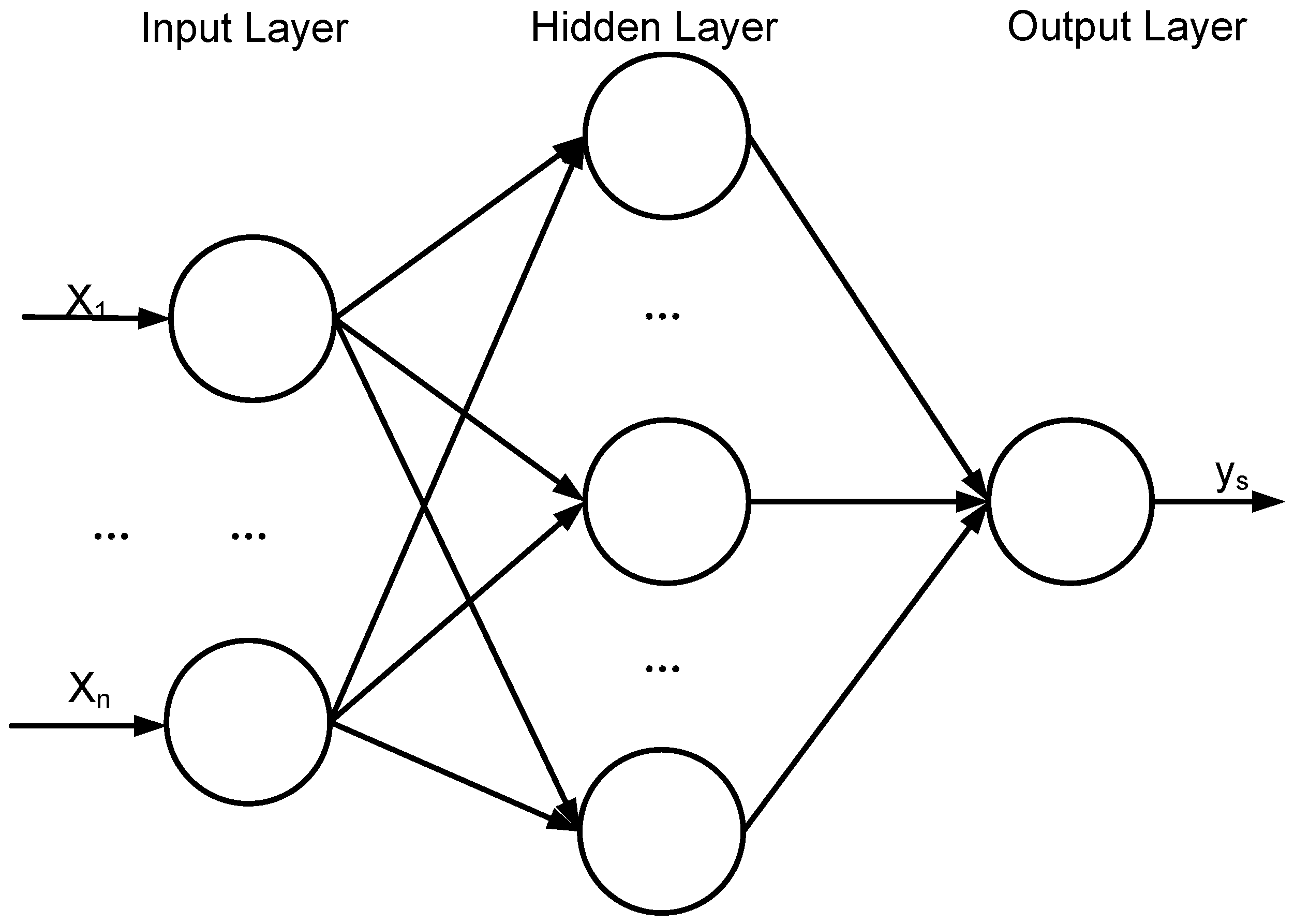
ELM is a kind of SLFNs. The diagram of ELM is shown in Figure 1. Consider N distinct samples $(x_i,t_i)$, if ELM with L hidden nodes and activation function $g(\cdot )$ can approximate the target with zero errors, it can be modeled by

$$t_i={\displaystyle \sum _{j=1}^L{\beta }_{j}g(w_j\cdot x_i+b_j)}i=1,\dots ,N$$

(1)

where ${\beta }_j$ is the output weight vector, $b_j$ is the hidden bias vector, $w_j$ is the input weight vector, $t_i$ is the target output vector, and $x_i$ are inputs vector.

The compact form of Equation (1) can be rewritten by

$$T=H\beta$$

(2)

where $T=[t_1,t_2,\cdots ,t_N]$, $\beta =[{\beta }_1,{\beta }_2,\cdots ,{\beta }_L]$, $H$ is called the hidden layer output matrix, and can be defined as

$$H={\left[\begin{array}{ccc}g(w_1\cdot x_1+b_1)& \cdots & g(w_L\cdot x_1+b_L)\\ \cdots & \cdots & \cdots \\ g(w_1\cdot x_N+b_1)& \cdots & g(w_L\cdot x_N+b_L)\end{array}\right]}_{N\times L}$$

(3)

Normally, the number of hidden nodes is less than the number of the training sample, the target is hard to approximated by ELM with zero errors. In ELM, the input weights and the hidden bias are randomly determined. After given $w_j$ and $b_j$, the output weight vector can be analytically calculated by a least squares method, and the special solution can be expressed as

$$\beta *=H^{+}Y$$

(4)

where $H^{+}$ is the generalized Moore Penrose inverse of $H$.

ELM exhibits many significant properties, which make it became a type of appealing SLFN approach. First, ELM presents very fast learning speed since its network parameters is determined by the way of iterative free. Second, ELM uses a least squares method to approach the training sample, and the smaller training error can be obtained. In addition, ELM overcomes the many problems faced by traditional NNs, such as local minima, the overtraining, learning rate, and so on.

2.2. Improved DE

Differential evolution algorithm (DE) is proposed by Storn and Price as a kind of population optimization algorithm and it is widely used in nonlinear and complex optimization problems [35]. The basic steps of DE can be described as follows:

(1) Initialization: given a set of vector $x_{iG}^D$, (i = 1, 2, …, NP). NP is the number of population. D is the dimension of each population. For each individual population, the Gth generation vectors can be expressed by

$$x_{i,G}^D=[x_{i,G}^D,\dots ,x_{NP,G}^D]$$

(5)

(2) Mutation: a mutation vector can be defined as

$$v_{i,G+1}^D=x_{r1,G}^D+F\times (x_{r2,G}^D-x_{r3,G}^D)$$

(6)

where $v_{i,G+1}^D$ is called a the G+1th generation mutation vector, $r_1$, $r_2$, $r_3\in$ [1, 2, …, NP] and $r_1\ne r_2\ne r_3\ne i$. F is Scaling factor, which is a constant factor and is used for scaling the difference vectors, its value usually is chosen during [0.4, 1].

(3) Crossover: in this step, a Gth generation trial vector can be expressed as

$$u_{i,G}^D=(u_{i,G}^1,u_{i,G}^2,\dots ,u_{i,G}^D)$$

(7)

Then, a G+1th generation trial vector can be formed as

$$u_{i,G+1}^j=\{\begin{array}{ll}{\nu }_{i,G}^j& \mathrm{if}rand\le C\mathrm{or}j=j_r\\ x_{i,G}^j& \mathrm{otherwise}\end{array}$$

(8)

where C is a random number in [0, 1] and called crossover rate. $j_r$ is denoted a dimensional index and randomly chosen in [1, D].

(4) Selection: the selection process is defined as

$$x_{i,G+1}^D=\{\begin{array}{ll}{u}_{i,G}^D& \mathrm{if}f(u_{i,G}^D)>f(x_{i,G}^D)\\ x_{i,G}^D& \mathrm{otherwise}\end{array}$$

(9)

where the f(.) is the fitness function.

The original DE has a good performance for global search, but its convergence speed is slow. To overcome this limitation, the mutation vector is replaced by [35]

$$v_{i,G+1}^D=x_b+F\times (x_{r2,G}^D-x_{r3,G}^D)$$

(10)

where $x_b$ is denoted the best individual in the population.

In order to improve the balance between global and local search ability, the Gth generation constant fact $F_G$ can be replaced as

$$F_G=2.0\times F_{rG}-1.0$$

(11)

where $F_{rG}$ is randomly chosen in [0,1]. The trial vector can be expressed by

$$v_{i,G+1}=x_b+F_G\times (x_{r2,G}-x_{r3,G})$$

(12)

2.3. PIs Construction and Assessment

2.3.1. PI Formulation

Given a training data sample $D=\left\{{(x_i,t_i)}_{i=1}^N\right\}$, $x_i$ is an input dataset that include historical information (solar power, wind speed, wind direction, ambient temperature, cell temperature, solar irradiance). $t_i$ is five minutes ahead PV power, which is used as the target. PIs are constructed to cover the target $t_i$ with the prescribed confidence level $(1-\alpha )$, named as PI nominal confidence (PINC) $100(1-\alpha )\%$, for the i-th target, the PIs $G_t^{\alpha }(x_i)$ can be defined as

$$G(x_i)=[L(x_i),U(x_i)]$$

(13)

where $L(x_i)$ and $U(x_i)$ denote the lower and upper bounds of PIs, respectively. The coverage rate of PIs can be described as

$$P(t_i\in [L(x_i),U(x_i)])=100(1-\alpha )\%$$

(14)

The $t_i$ is the i-th measured target, it can be defined as

$$t_i=y(x_i)+\mu (x_i)=f(x_i,\vartheta )+\epsilon (x_i)$$

(15)

where $y(x_i)$ is mean of true regression and $\epsilon (x_i)$ mean of noise with zero mean. $f(x_i,\vartheta )$ describes a mapping between input $x_i$ and true regress value $y(x_i)$. In this paper, ELM algorithm is chosen as a regression model to approach the true regress value. Therefore, the mean of the true regress $y(x_i)$ can be approximate with output of ELM model $f(x_i,\widehat{\vartheta })$

$$\widehat{y}(x_i)=f(x_i,\widehat{\vartheta })=E(t_i/x_i)$$

(16)

where $\widehat{y}(x_i)$ represents prediction value of target, the prediction error can be defined as

$$t_i-\widehat{y}(x_i)=[y(x_i)-\widehat{y}(x_i)]+\epsilon (x_i)$$

(17)

where $t_i-\widehat{y}(x_i)$ means the total prediction error and denotes the error between measure value $t_i$ and real estimate value $\widehat{y}(x_i)$. The $[y(x_i)-\widehat{y}(x_i)]$ denotes the error between the expectation true regress output and actual ELM output. $\epsilon (x_i)$ denotes the noise with zero mean. PIs are constructed to quantify the uncertainties by the total prediction, which consist of two independence statistical parts: $[y(x_i)-\widehat{y}(x_i)]$ and $\epsilon (x_i)$. Therefore, the total variance can be defined as

$${\sigma }_t^2(x_i)={\sigma }_{\widehat{y}}^2(x_i)+{\sigma }_{\epsilon }^2(x_i)$$

(18)

where ${\sigma }_{\widehat{y}}^2(x_i)$ is the variance of model uncertainties and ${\sigma }_{\epsilon }^2(x_i)$ is the variance of data uncertainties. The low bound $L_t^{\alpha }(x_i)$ and upper bound $U_t^{\alpha }(x_i)$ can be rewritten as

$$L_t^{\alpha }(x_i)=\widehat{y}(x_i)-z_{1-\alpha /2}\sqrt{{\sigma }_{\widehat{t}}^2(x_i)}$$

(19)

$$U_t^{\alpha }(x_i)=\widehat{y}(x_i)+z_{1-\alpha /2}\sqrt{{\sigma }_{\widehat{t}}^2(x_i)}$$

(20)

where $z_{1-\alpha /2}$ is the $1-\alpha /2$ quantile of standard normal distribution.

2.3.2. Metrics for PIs Quality

The PIs coverage probability (PICP) and PIs’ width is two key indicators. To assess the quality of PIs, several metrics and indicators are introduced.

PICP is the most important indicator to assess reliability of PIs, whose value indicates probability level that PIs cover the future target. Larger PICP value indicates that the PIs have a greater probability of coverage target. For the N training samples, the PICP can be defined as

$$\mathrm{PICP}=\frac{1}{N}{\displaystyle \sum _t^N{\delta }_t}$$

(21)

where ${\delta }_t$ is a Boolean value which can be expressed as

$${\delta }_t=\{\begin{array}{ll}1,& t_i\in G_i^{\alpha }\\ 0,& t_i\notin G_i^{\alpha }\end{array}$$

(22)

The interval width is other very important indicator evaluate the quality of PIs. If interval width is ignored, we only take the PICP into account, and even the high PICP value has been obtained, then decision-maker is also difficult to obtain useful forecasting information. Therefore, a higher quality PIs should fully consider PICP and sharpness of PIs. Mean prediction interval width (MPIW) can be used to quantify the sharpness of PIs.

$$\mathrm{MPIW}=\frac{1}{NR}{\displaystyle \sum _{i=1}^N(U_t^{\alpha }(x_i)-L_t^{\alpha }(x_i))}$$

(23)

where the R is the target range, N is the number of test dataset.

2.4. Traditional Bootstrap Method for PIs Construction

2.4.1. Variance of Model Uncertainty

The bootstrap method, a resampling technique, is introduced and named in 1979 [36]. Due to its advantages of simplicity and robustness, it is widely used to estimate almost unknown distribution by an empirical distribution. In regression application, bootstrap methods are applied to estimate uncertainties of regression models [19]. In this paper, it is used to estimate the uncertainties of the ELM model, which is caused by structure misspecification and randomly given input parameters. The variance is used to represent model uncertainties.

For the paired bootstrap method, an original training data sample is defined as $D_{orin}={\{(x_i,t_i)\}}_{i=1}^N$, the B training sub-datasets $D_{sub}={\{(x_i,t_i)\}}_{i=1}^{N*}$ are uniformly re-sampled from $D_{orin}$ with replacement. The output of each ELM model is ${\widehat{y}}_s(x_i)$. The true regression value can be approximated by the mean of the bootstrap ELMs outputs. For B ELM models, it can be can be expressed as

$$\widehat{y}(x_i)=\frac{1}{B}{\displaystyle \sum _{s=1}^B{\widehat{y}}_s(x_i)}$$

(24)

The variance can be used to quantify the uncertainties of ELM models, based on the B times ELM estimated results, the variance of model uncertainties can be written as

$${\sigma }_{\widehat{y}}^2(x_i)=\frac{1}{B-1}{\displaystyle \sum _{s=1}^B({\widehat{y}}_s(x_i)-\widehat{y}(x_i))}$$

(25)

2.4.2. Variance of Data Noise

The uncertainties of regression model and residual noise are combined to construct the PIs. After determining the variance of the model uncertainties, the variance of data noise ${\sigma }_{\epsilon }^2(x_i)$ also should be estimated to construct PIs. Based on Equation (17), the total variance ${\sigma }_t^2(x_i)$ can be rewritten as

$${\sigma }_t^2(x_i)=E[{(t_i-\widehat{y}(x_i))}^2|x_i]$$

(26)

According to Equations (18) and (26), the variance of data noise can be expressed as

$${\sigma }_{\epsilon }^2(x_i)={\sigma }_t^2(x_i)-{\sigma }_{\widehat{y}}^2(x_i)=E[{(t_i-\widehat{y}(x_i))}^2|x_i]-{\sigma }_{\widehat{y}}^2(x_i)$$

(27)

Equation (27) shows relationship between ${\sigma }_{\epsilon }^2(x_i)$ and $x_i$. Therefore, a regression model can be used to fit ${\sigma }_{\epsilon }^2(x_i)$ with input $x_i$. The squared residual error can be expressed as

$$r^2(x_i)=\max ({[t_i-\widehat{y}(x_i)]}^2)-{\widehat{\sigma }}_{\widehat{y}}^2(x_i),0)$$

(28)

where the $\widehat{y}(x_i)$ and ${\widehat{\sigma }}_{\widehat{y}}^2(x_i)$ can be obtained from Equations (24) and (26), respectively. The residual errors and the corresponding the inputs can be built a new dataset as

$$D_{r^2}={\{x_i,r^2(x_i)\}}_{i=1}^N$$

(29)

Data noise can be supposed to a normally distributed with zero mean [19]. Based on the normal assumption in Equation (28), it can be defined as

$$P(r^2(x_i);{\widehat{\sigma }}_{\epsilon }^2(x_i))=\frac{1}{\sqrt{2\pi {\widehat{\sigma }}_{\epsilon }^2(x_i)}}\exp (-\frac{r^2(x_i)}{2{\widehat{\sigma }}_{\epsilon }^2(x_i)})$$

(30)

Noise variance is a kind of effective formulation to approximate the noise uncertainty of PV data. A separate ELM model is used to estimate the unknown noise ${\sigma }_{\epsilon }^2(x_i)$, the parameters of ELM is trained to maximize the probability for the new samples in $D_{r^2}$. Minimizing the negative value of a variable is equivalent to maximizing the positive value of a variable, therefore, after ignoring the constant part in Equation (30), the cost function for training the ELM model can be obtained and defined as

$$C_{ML}=\frac{1}{2}{\displaystyle \sum _{i=1}^n(\ln ({\sigma }_{\epsilon }^2(x_i))+\frac{r^2(x_i)}{{\sigma }_{\epsilon }^2(x_i)})}$$

(31)

Since the variance is always positive, the sigmoid function selected as activation function of the ELM. The evolutional algorithm can be applied to optimize the parameters of ELM (ELM_MLE) by minimizing the cost function Equation (31).

After obtaining both ${\sigma }_{\epsilon }^2(x_i)$ and ${\sigma }_{\widehat{y}}^2(x_i)$, the PIs can be construct according to Equations (19) and (20) with the confidence level.

3. Proposed Method

For the traditional bootstrap method, the variance of noise is estimated based on the assumption that the data noise is normally distributed with zero mean [19]. The cost function of maximum likelihood estimation is used to train the ELM parameters, rather than the one is defined by using evaluation indicators of the overall PIs performance. Therefore, the traditional PIs cannot always obtain optimal PIs. To solve this issue, in this paper, a novel PI based cost function, which takes the PICP and interval width into account, is proposed to obtain variance of data noise.

3.1. PIs Based Cost Function

Performance evaluation of PIs should include two aspects: both MPIW and PICP. It is meaningless if the performance of PIs is revealed only by one aspect. A PI based cost function, named coverage width based criterion (CWC) is defined as

$$\mathrm{CWC}=\mathrm{MPIW}+{\gamma }_{\mathrm{PICP}}\lambda \times \left|\mu -\mathrm{PICP}\right|$$

(32)

where $\mu$ denotes the prescribed probability, equal to the PIs nominal confidence (PINC) level $100(1-\alpha )\%$. $\lambda$ is a hyper-parameter and its value is set between 10 and 100 to penalize the invalid PIs, and ${\gamma }_{\mathrm{PICP}}$ is a function of PICP. If the value of PICP is more than $\mu$, the ${\gamma }_{\mathrm{PICP}}$ value will be set to 0, and the value of CWC is determined by MPIW. This means that the PIs’ width will be maintained. Whereas, if the value of PICP is less than $\mu$, the ${\gamma }_{\mathrm{PICP}}$ value will be set to 1, and the CWC is the sum of both MPIW and $\lambda \ast \left|\mu -\mathrm{PICP}\right|$, this indicates that the wider PIs should be obtained to get more suitable the PICP value. The CWC value is normalized by nominal PV power and its value is expressed as a percentage in this paper. If a smaller CWC value is obtained at the given confidence level $100(1-\alpha )\%$, a better performing PI has been achieved.

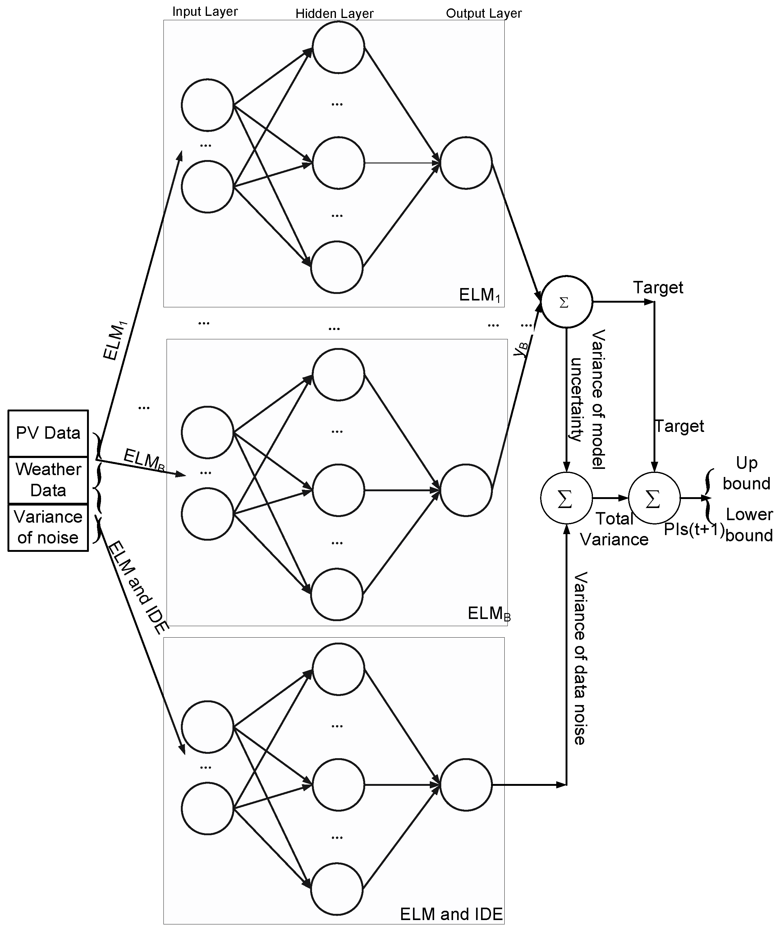
As shown in Figure 2, the proposed PIs are constructed by combining the variance of both the model uncertainties and data noise. To obtain optimal PIs, it is critical to obtain the accurate estimation variance of data noise. In this study, an ELM model is developed to estimate the variance of data noise and the improved DE (IDE) is employed to optimize parameters of ELM model by minimizing the CWC. Therefore, based on the Equation (32), the PI based objective function is proposed for IDE as follow:

$$F=\mathrm{Minimize}\left(\mathrm{CWC}\right)$$

(33)

The constraints can be defined as

$$U(x)>L(x)\ge 0$$

(34)

$$\{\begin{array}{l}\mathrm{if}{\alpha }_i\le {\alpha }_j\\ L^{{\alpha }_i}(x)\ge L^{{\alpha }_j}(x)\mathrm{and}{U}^{{\alpha }_i}(x)\ge U^{{\alpha }_j}(x)\end{array}$$

(35)

For the two constraints, the first one is automatically satisfied as long as the calculation is correct. The other one indicates that when smaller confidence level $(1-\alpha )$ is set for the same datasets, the narrower PIs should be obtained.

3.2. Overall Procedures

Generally, the proposed technique can be divided into two stages. The detail process can be defined as follows.

The first stage, the bootstrap technique is used to estimate variance of model uncertainties.

Step (1) resample B training samples $D_{sub}={\{(x_i,t_i)\}}_{i=1}^{N*}$ with replacement from the original PV training dataset $D_t={\{(x_i,t_i)\}}_{i=1}^N$.

Step (2) ELM regress model is used to estimate each training sample and obtain ${\{{\widehat{y}}_s(x_i)\}}_{s=1}^B$.

Step (3) Based on step 2, the mean output of B ELMs models $\widehat{y}(x_i)$ and variance of model uncertainty ${\sigma }_y^2(x_i)$ are calculated by Equations (23) and (24), respectively.

Step (4) residual sample $D_{r^2}={\{x_i,r^2(x_i)\}}_{i=1}^N$ is built by the Equation (27).

The aim of the second stage is to estimate the variance of data noise and to construct optimal PIs.

An ELM model is used to estimate variance of data noise. Since the input weights and hidden biases of ELM are randomly given, it is unavoidable that some of them are non-optimal parameters. Moreover, it is proved that performance of ELM relies on the quality of input weights and hidden biases [32]. In this paper, to obtain the optimal PIs, the IDE algorithm is used to find the optimal ELM parameters (input weights and biases) by minimizing the PIs based cost function.

Step (1), randomly generate the population, and the candidate solution $v_i$ is composed of a set of input weights and hidden biases, the i-th individual can be express as

$$v_i=[w_{11},\cdots ,w_{1L},w_{21},\cdots ,w_{2L},\cdots ,w_{n1},w_{nL},b_1,\cdots ,b_n]$$

(36)

Step (2), each individual population consist of a set of weights and hidden biases. The corresponding output weights are calculated by using Equation (2), and ${\widehat{\sigma }}_{\epsilon }^2(x_i)$ is estimated.

Step (3), calculate the total variance ${\widehat{\sigma }}_t^2(x_i)$ based on Equation (18), and calculate low bound ${\widehat{L}}_t^{\alpha }(x_i)$ and upper bound ${\widehat{U}}_t^{\alpha }(x_i)$ based on Equation (19) and Equation (20), respectively.

Step (4), the fitness cost function the CWC can be calculated based on Equation (32), Equation (21) and Equation (23).

Step (5), improved ID algorithm is developed to adjust ELM parameters for obtain the optimal ${\widehat{\sigma }}_{\epsilon }^2(x_i)$ based on objective function Equation (33) and constraints Equation (34).

Step (6), the PIs is constructed based on step 5 and step 3.

4. Experimental Analysis

4.1. Experimental Data Description

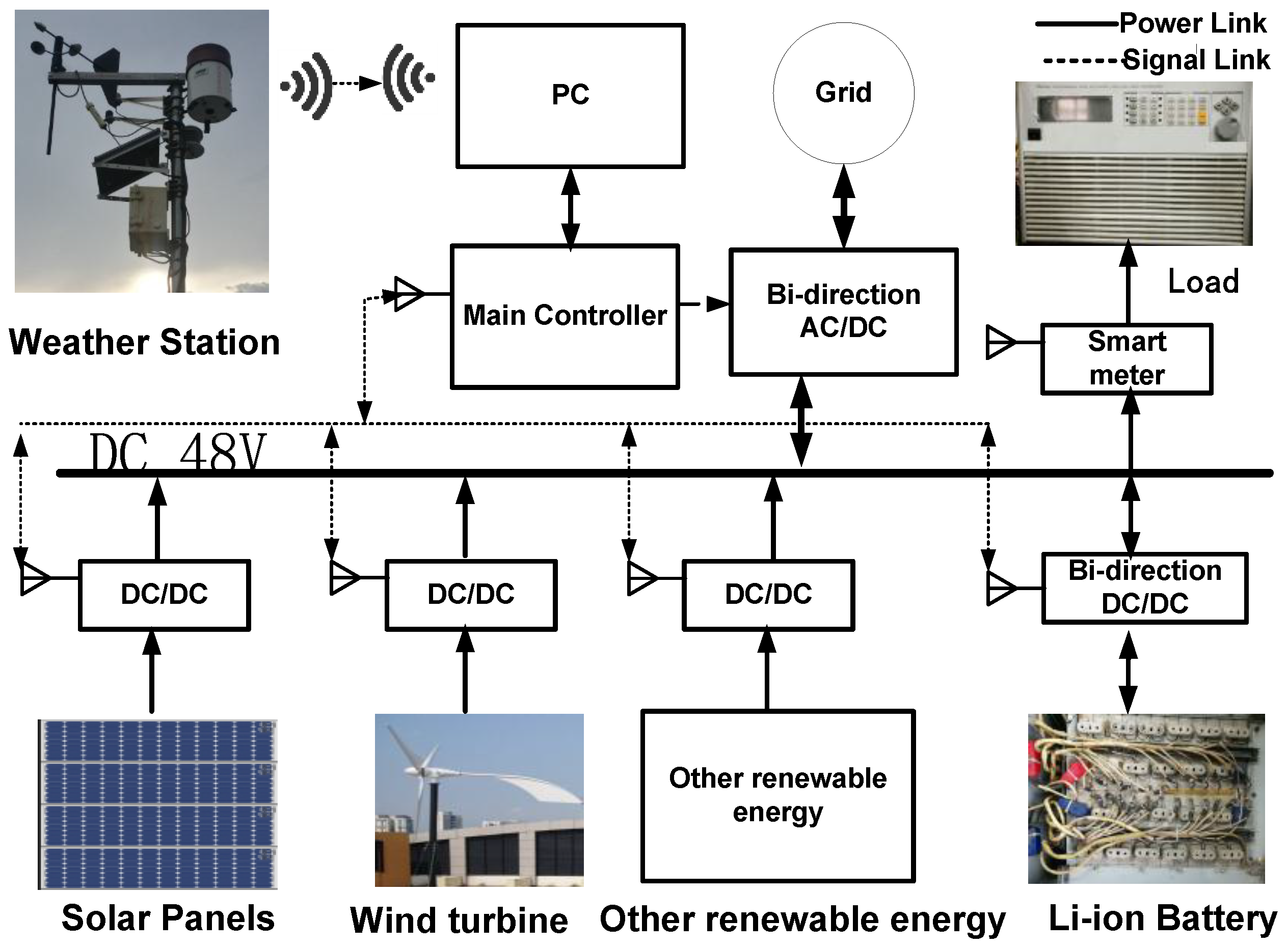
The proposed method in this study has been tested by actual historical PV and meteorological data, which were measured from a laboratory-scale DC micro-grid system (at Singapore Polytechnic (1.35 N, 103.68 E and 41 m elevation above the sea level). As shown in Figure 3, the DC micro-grid system can operate on grid model and off grid model. The maximum operation power of rooftop PV system 1 kW, which is constituted by a series of four solar panels (CSP6P-250). The weather information is collected by the weather station (HOBO weather station). The web box monitors and stores the measured data including solar radiation, ambient temperature, PV module temperature, wind speed, and PV output power. The DC micro-grid system operates with no gap and sampling time resolution of measured data is 5 min. The data time (7:00 to 19:00) are used to construct the dataset from January 2013 until December 2014.

4.2. Experimental Results and Analysis

To evaluate the proposed approach, the persistence method [37], MLE-Bootstrap method [19], double bootstrap method [34], and bootstrap based traditional NNs (BNN) approach [29] are used for benchmarking the forecasting performance of solar power. The persistence ensemble (PeEn) method is used to construct PIs for PV power, of which the forecast errors are assumed to be randomly and normally distributed [37]. Its mean is derived from the 10 last available power measurements, and the variance is computed using the 10 latest observations. The MLE-Bootstrap method and Double bootstrap method, and our proposed the method are all used ELM as regress model. The regress model of BNN approach is traditional NNs. MLE-Bootstrap approach [19] obtains the variance of data noise by using maximum-likelihood cost function, (MLE-Bootstrap). Double bootstrap methods (Double-Bootstrap) proposed in [34], and the variance of data noise is also obtained by using a bootstrap model. BNN approach obtains the variance of data noise using the cost function same as our proposed method. In this study, the number of bootstrap replicates is 100 for MLE-Bootstrap method, double bootstrap method, BNN approach and proposed method. They are all operating on a PC with Intel Core i7-2670QM, CPU @2.2 GHz. For power system operation, if we can obtain forecasted information of high confidence levels, it is more helpful to reduce the risks. Therefore, in this study, the proposed method is tested at different high confidence levels (90%, 95%, and 99%).

The level of uncertainties in PV power generation has a strong correlation to chaotic climate systems. The weather conditions and the patterns of solar radiation vary greatly in different seasons. Singapore has a tropical climate and its climate is characterized by two monsoon seasons separated by inter-monsoonal periods. To verify the performance of the proposed approach, four periods in Singapore: northeast monsoon season (December to March), inter-monsoon period (April to May), southwest monsoon season (June to September), and inter-monsoon period (October–November) are investigated, respectively. In each season, the corresponding model is developed. When considering the seasonal difference and diversity, Northeast monsoon 2013, the Inter monsoon (Northeast monsoon to southeast monsoon NS) 2013, southeast monsoon 2013, and inter monsoon (Southeast monsoon to northeast monsoon, SN) 2013 are selected to constructed test dataset to verify the proposed the approach, and remain data are used as training dataset.

As shown in

Table 1. Performance comparison of various constructed PIs in different seasons.

Seasons	PINC	Value	Persistence	BNN	Double Bootstrap	MLE Bootstrap	Proposed Bootstrap
Northeast monsoon	90%	PICP	76.74	94.65	93.75	94.10	94.79
		MPIW	19.01	13.19	17.83	16.90	12.53
	95%	PICP	79.86	96.21	95.28	95.93	96.38
		MPIW	26.83	17.21	20.57	20.32	15.26
	99%	PICP	83.98	98.35	96.75	98.32	98.79
		MPIW	37.12	18.92	20.82	22.90	18.53
Inter monsoon (NS)	90%	PICP	75.35	93.13	91.35	92.71	93.06
		MPIW	14.88	12.57	15.70	13.88	12.38
	95%	PICP	77.39	96.23	94.35	95.65	96.12
		MPIW	24.71	14.92	18.12	16.15	14.84
	99%	PICP	78.81	98.50	96.78	97.69	98.52
		MPIW	35.36	17.67	21.26	19.73	17.32
Southwest monsoon	90%	PICP	78.82	92.95	90.63	91.67	93.06
		MPIW	20.06	13.64	17.62	15.77	13.35
	95%	PICP	78.82	95.72	94.63	95.21	95.98
		MPIW	26.06	16.59	20.15	18.59	16.23
	99%	PICP	78.82	97.36	90.63	91.67	97.25
		MPIW	34.06	20.12	23.27	21.14	19.80
Inter monsoon (SN)	90%	PICP	75.27	92.68	89.93	90.28	92.71
		MPIW	26.54	13.25	17.66	14.09	12.57
	95%	PICP	76.93	95.57	94.93	95.28	95.62
		MPIW	36.57	15.89	20.95	17.38	15.83
	99%	PICP	78.56	98.65	97.93	97.28	98.71
		MPIW	46.51	19.53	22.16	20.17	19.13

and Figure 4, the proposed approach always exceeds the persistence method, the double bootstrap method, and MLK bootstrap method. The larger PICP value is obtained than the corresponding nominal confidence. It indicates that the PIs, which has a higher probability of covering the 5 min ahead, PV power than the expected value. When compared to the other benching models, the proposed method obtained the greatest PICP value. Moreover, the MPIW value of the proposed approach is smaller than other benchmarking models. It indicates that the proposed method achieved narrower intervals.

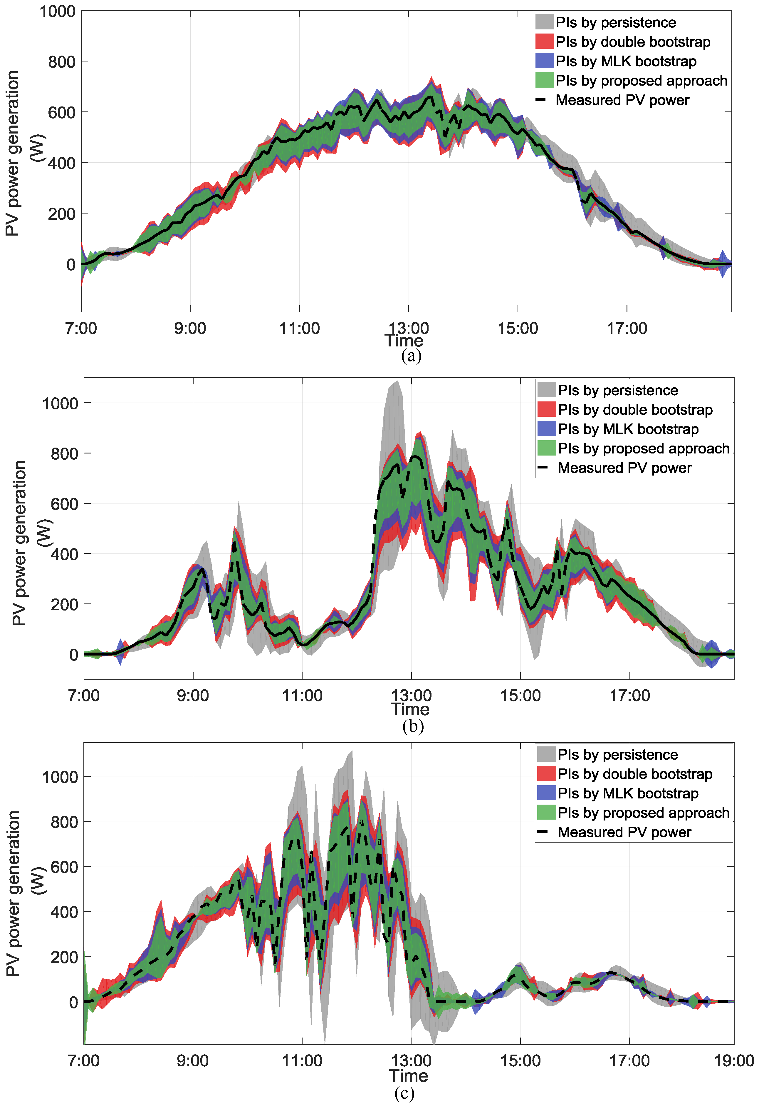
To further evaluate the effectiveness and applicability of the proposed approach under different weather conditions, the three typical daily weather types are selected (sunny conditions, cloudy conditions, and thunderstorm). The experimental results of the proposed method and four benchmarking models are shown in Figure 5 and

Table 2. Performance comparison of various constructed prediction intervals (PIs) under different weather conditions.

Weather conditions	PINC	Value	Persistence	BNN	Double Bootstrap	MLE Bootstrap	Proposed Bootstrap
Sunny	90%	PICP	88.89	95.03	94.44	93.75	95.14
		MPIW	8.00	6.96	9.72	8.53	6.81
	95%	PICP	89.83	97.10	96.15	96.58	97.14
		MPIW	16.12	12.15	15.81	13.87	11.76
	99%	PICP	91.65	98.93	97.64	98.15	98.87
		MPIW	23.25	15.96	19.63	18.52	15.95
Cloudy	90%	PICP	81.94	93.15	92.36	93.06	93.18
		MPIW	17.55	9.79	14.94	11.76	9.83
	95%	PICP	83.94	96.68	95.03	95.37	96.79
		MPIW	31.55	15.89	19.12	16.19	15.83
	99%	PICP	84.94	98.35	96.36	97.01	98.25
		MPIW	39.65	16.57	23.06	19.76	16.23
Thunderstorm	90%	PICP	78.47	90.87	90.07	90.28	90.97
		MPIW	19.74	10.96	15.90	13.17	10.88
	95%	PICP	81.63	95.50	94.86	95.28	95.96
		MPIW	39.74	16.70	20.14	18.20	16.65
	99%	PICP	84.57	98.15	96.39	96.28	98.03
		MPIW	48.74	21.94	25.51	23.17	21.72

. The proposed method achieves a greater PICP value in three weather conditions than the benchmark models. When the confidence level is 90%, the proposed method generates the PICP 95.14% in sunny conditions, 93.18% in cloudy conditions, and 90.07% in thunderstorm. Furthermore, the proposed method obtains the narrower PIs width than other methods, especially for the persistence method.

As shown in Figure 4 and Figure 5, Table 2 and

Table 3. The average training time and test time comparison.

Method	Training Time (s)	Test Time (s)
BNN Bootstrap	8579.32	5.730
MLE Bootstrap	138.67	0.425
Double Bootstrap	147.19	0.836
Proposed Bootstrap	135.53	0.421

, the BNN approach and the proposed approach have relatively comparable performance. The BNN approach also can achieve much better quality PIs than the persistence method, MLK bootstrap method and Double bootstrap under different weather conditions and seasons. This is not hard to understand that BNN approach has relatively close performance to the proposed method, because the NNs have good nonlinear mapping capability. However, the traditional NNs have the significant disadvantage of high computational burden. As shown in Table 3, the training time is the average time of training 30 days dataset and the test time is the average time of testing one day dataset. The proposed hybrid approach, Double Bootstrap approach, and MLE Bootstrap approach all perform more than 60 times faster than the BNNs approach, and it demonstrates that the ELM based bootstrap method has a significantly higher efficiency. The training time of proposed approach is slightly faster than Double approach, it indicates the number of iterations of DE is less than the number of bootstrap replicates number.

5. Conclusions

Solar power short term forecasting is crucial to power system operation and economic cost. In this paper, a novel short term PIs forecasting approach is proposed for uncertainties quantification of PV power generation by using extreme learning machine and bootstrap technique. The uncertainties of both data noise and the regression model are used to construct PIs. The bootstrap technique is used to estimate uncertainties of ELM models, and a hybrid model of ELM and IDE with PIs best cost function is proposed for quantifying the uncertainties of data noise. The proposed method is tested under different seasons conditions and three different weather conditions by using actual lab-scale PV micro-grid data. When compared to both MLE-bootstrap and Double-bootstrap approach, experimental results show the proposed method significantly improves the quality of the PIs for five-minute-ahead short term PV power forecasting. Due to the fast learning speed of ELM, the proposed approach can be more than 60 times faster in the training process and be 10 times faster in the test process than BNNs approach, which indicates that the proposed method has a high online application potential for short-term PV power generation forecasting in future.

References

- Simoes, S.; Zeyringer, M.; Mayr, D.; Huld, T.; Nijs, W.; Schmidt, J. Impact of different levels of geographical disaggregation of wind and PV electricity generation in large energy system models: A case study for Austria. Renew. Energy 2017, 105, 183–198. [Google Scholar] [CrossRef]
- Bracale, A.; Caramia, P.; Carpinelli, G.; Fazio, A.R.D.; Ferruzzi, G. A bayesian method for short-term probabilistic forecasting of photovoltaic generation in smart grid operation and control. Energies 2013, 6, 733–747. [Google Scholar] [CrossRef]
- Zhang, J.; Florita, A.; Hodge, B.M.; Lu, S.; Hamann, H.F.; Banunarayanan, V.; Brockway, A.M. A suite of metrics for assessing the performance of solar power forecasting. Sol. Energy 2015, 111, 157–175. [Google Scholar] [CrossRef]
- Yao, E.; Samadi, P.; Wong, V.W.S.; Schober, R. Residential demand side management under high penetration of rooftop photovoltaic units. IEEE Trans. Smart Grid 2016, 7, 1597–1608. [Google Scholar] [CrossRef]
- Wan, C.; Zhao, J.; Song, Y.; Xu, Z.; Lin, J.; Hu, Z. Photovoltaic and solar power forecasting for smart grid energy management. CSEE J. Power Energy Syst. 2015, 1, 38–46. [Google Scholar] [CrossRef]
- Bae, K.Y.; Han, S.J.; Dan, K.S. Hourly solar irradiance prediction based on support vector machine and its error analysis. IEEE Trans. Power Syst. 2017, 32, 935–945. [Google Scholar] [CrossRef]
- Bracale, A.; Carpinelli, G.; Falco, P.D. A probabilistic competitive ensemble method for short-term photovoltaic power forecasting. IEEE Trans. Sustain. Energy 2016, 8, 551–560. [Google Scholar] [CrossRef]
- Han, S.J.; Bae, K.Y.; Park, H.S.; Dan, K.S. Solar power prediction based on satellite images and support vector machine. IEEE Trans. Sustain. Energy 2016, 7, 1255–1263. [Google Scholar]
- Bacher, P.; Madsen, H.; Nielsen, H.A. Online short-term solar power forecasting. Sol. Energy 2009, 83, 1772–1783. [Google Scholar] [CrossRef] [Green Version]
- Huang, C.M.; Chen, S.J.; Yang, S.P.; Kuo, C.J. One-day-ahead hourly forecasting for photovoltaic power generation using an intelligent method with weather-based forecasting models. IET Gener. Transm. Distrib. 2015, 9, 1874–1882. [Google Scholar] [CrossRef]
- Asrari, A.; Wu, T.X.; Ramos, B. A hybrid algorithm for short-term solar power prediction—Sunshine state case study. IEEE Trans. Sustain. Energy 2017, 8, 582–591. [Google Scholar] [CrossRef]
- Golestaneh, F.; Pinson, P.; Gooi, H.B. Very short-term nonparametric probabilistic forecasting of renewable energy generation—With application to solar energy. IEEE Trans. Power Syst. 2016, 31, 3850–3863. [Google Scholar] [CrossRef]
- Bludszuweit, H.; Dominguez-Navarro, J.A.; Llombart, A. Statistical analysis of wind power forecast error. IEEE Trans. Power Syst. 2008, 23, 983–991. [Google Scholar] [CrossRef]
- Wan, C.; Lin, J.; Song, Y.; Xu, Z.; Yang, G. Probabilistic forecasting of photovoltaic generation: An efficient statistical approach. IEEE Trans. Power Syst. 2016, 32, 2471–2472. [Google Scholar] [CrossRef]
- Sperati, S.; Alessandrini, S.; Monache, L.D. An application of the ECMWF ensemble prediction system for short-term solar power forecasting. Sol. Energy 2016, 133, 437–450. [Google Scholar] [CrossRef]
- Khosravi, A.; Nahavandi, S.; Creighton, D.; Atiya, A.F. Lower upper bound estimation method for construction of neural network-based prediction intervals. IEEE Trans. Neural Netw. 2011, 22, 337–346. [Google Scholar] [CrossRef] [PubMed]
- Wan, C.; Lin, J.; Wang, J.; Song, Y.; Dong, Z.Y. Direct quantile regression for nonparametric probabilistic forecasting of wind power generation. IEEE Trans. Power Syst. 2016, 32, 2767–2778. [Google Scholar] [CrossRef]
- Shrivastava, N.A.; Khosravi, A.; Panigrahi, B.K. Prediction interval estimation of electricity prices using pso-tuned support vector machines. IEEE Trans. Ind. Inform. 2015, 11, 322–331. [Google Scholar] [CrossRef]
- Wan, C.; Xu, Z.; Wang, Y.; Dong, Z.Y.; Wong, K.P. A hybrid approach for probabilistic forecasting of electricity price. IEEE Trans. Smart Grid 2014, 5, 463–470. [Google Scholar] [CrossRef]
- Zhang, G.; Wu, Y.; Wong, K.P.; Xu, Z.; Dong, Z.Y.; Iu, H.C. An advanced approach for construction of optimal wind power prediction intervals. IEEE Trans. Power Syst. 2015, 30, 2706–2715. [Google Scholar] [CrossRef]
- Li, S.; Goel, L.; Wang, P. An ensemble approach for short-term load forecasting by extreme learning machine. Appl. Energy 2016, 170, 22–29. [Google Scholar] [CrossRef]
- Lorenz, E.; Hurka, J.; Heinemann, D.; Beyer, H.G. Irradiance forecasting for the power prediction of grid-connected photovoltaic systems. IEEE J. Sel. Top. Appl. Earth Obs. Remote Sens. 2009, 2, 2–10. [Google Scholar] [CrossRef]
- David, M.; Ramahatana, F.; Trombe, P.J.; Lauret, P. Probabilistic forecasting of the solar irradiance with recursive arma and garch models. Sol. Energy 2016, 133, 55–72. [Google Scholar] [CrossRef] [Green Version]
- Dong, Z.; Yang, D.; Reindl, T.; Walsh, W.M. Short-term solar irradiance forecasting using exponential smoothing state space model. Energy 2013, 55, 1104–1113. [Google Scholar] [CrossRef]
- Rana, M.; Koprinska, I.; Agelidis, V.G. 2d-interval forecasts for solar power production. Sol. Energy 2015, 122, 191–203. [Google Scholar] [CrossRef]
- Kavousi-Fard, A.; Khosravi, A.; Nahavandi, S. A new fuzzy-based combined prediction interval for wind power forecasting. IEEE Trans. Power Syst. 2016, 31, 18–26. [Google Scholar] [CrossRef]
- Ding, A.A. Prediction intervals for artificial neural networks. J. Am. Stat. Assoc. 1997, 92, 748–757. [Google Scholar]
- Ak, R.; Fink, O.; Zio, E. Two machine learning approaches for short-term wind speed time-series prediction. IEEE Trans. Neural Netw. Learn. Syst. 2015, 27, 1734–1747. [Google Scholar] [CrossRef] [PubMed]
- Khosravi, A.; Nahavandi, S.; Srinivasan, D.; Khosravi, R. Constructing optimal prediction intervals by using neural networks and bootstrap method. IEEE Trans. Neural Netw. Learn. Syst. 2015, 26, 1810–1815. [Google Scholar] [CrossRef] [PubMed]
- Huang, G.B.; Zhu, Q.Y.; Siew, C.K. Extreme learning machine: Theory and applications. Neurocomputing 2006, 70, 489–501. [Google Scholar] [CrossRef]
- Huang, G.B.; Zhou, H.; Ding, X.; Zhang, R. Extreme learning machine for regression and multiclass classification. IEEE Trans. Syst. Man Cybern. Part B Cybern. 2012, 42, 513–529. [Google Scholar] [CrossRef] [PubMed]
- Li, S.; Wang, P.; Goel, L. Short-term load forecasting by wavelet transform and evolutionary extreme learning machine. Electr. Power Syst. Res. 2015, 122, 96–103. [Google Scholar] [CrossRef]
- Chen, X.; Dong, Z.Y.; Meng, K.; Xu, Y.; Wong, K.P.; Ngan, H.W. Electricity price forecasting with extreme learning machine and bootstrapping. IEEE Trans. Power Syst. 2012, 27, 2055–2062. [Google Scholar] [CrossRef]
- Wan, C.; Xu, Z.; Pinson, P.; Dong, Z.Y.; Wong, K.P. Probabilistic forecasting of wind power generation using extreme learning machine. IEEE Trans. Power Syst. 2014, 29, 1033–1044. [Google Scholar] [CrossRef]
- Qin, A.K.; Huang, V.L.; Suganthan, P.N. Differential evolution algorithm with strategy adaptation for global numerical optimization. IEEE Trans. Evol. Comput. 2009, 13, 398–417. [Google Scholar] [CrossRef]
- Davison, A.C.; Hinkley, D.V. Bootstrap methods and their application. Technometrics 1997, 94, 216–217. [Google Scholar]
- Alessandrini, S.; Monache, L.D.; Sperati, S.; Cervone, G. An analog ensemble for short-term probabilistic solar power forecast. Appl. Energy 2015, 157, 95–110. [Google Scholar] [CrossRef]
Figure 1.
Diagram of ELM.
Figure 2.
Diagram of proposed approach.
Figure 3.
Experimental setup.
Figure 4.
The 5-min ahead PV power forecasting results of four seasons in Singapore: (a) northeast monsoon sunny conditions; (b) Inter monsoon (NS); (c) southwest monsoon; and, (d) Inter monsoon (SN) (PIs constructed by proposed model, double bootstrap, MLE-bootstrap and PeEn respectively) with 90% confidence level.
Figure 5.
The 5-min ahead photovoltaic (PV) power forecasting results of typical weather conditions: (a) sunny conditions; (b) cloudy conditions; and (c) thunderstorm (PIs constructed by proposed model, double bootstrap, MLK bootstrap and PeEn, respectively) with 90% confidence level.