Performance Assessment of Black Box Capacity Forecasting for Multi-Market Trade Application


1
Monitoring and Control Services, TNO, 9701 BK Groningen, The Netherlands
2
Faculty of Economics and Business, University of Groningen, 9700 AV Groningen, The Netherlands
3
Department of Electrical Engineering, University of Leuven, 3001 Leuven, Belgium
*
Author to whom correspondence should be addressed.
Energies 2017, 10(10), 1673; https://doi.org/10.3390/en10101673
Submission received: 28 August 2017
/
Revised: 17 October 2017
/
Accepted: 17 October 2017
/
Published: 23 October 2017
(This article belongs to the Special Issue Selected Papers from International Workshop of Energy-Open)
Abstract
:With the growth of renewable generated electricity in the energy mix, large energy storage and flexible demand, particularly aggregated demand response is becoming a front runner as a new participant in the wholesale energy markets. One of the biggest barriers for the integration of aggregator services into market participation is knowledge of the current and future flexible capacity. To calculate the available flexibility, the current aggregator pilot and simulation implementations use lower level measurements and device specifications. This type of implementation is not scalable due to computational constraints, as well as it could conflict with end user privacy rights. Black box machine learning approaches have been proven to accurately estimate the available capacity of a cluster of heating devices using only aggregated data. This study will investigate the accuracy of this approach when applied to a heterogeneous virtual power plant (VPP). Firstly, a sensitivity analysis of the machine learning model is performed when varying the underlying device makeup of the VPP. Further, the forecasted flexible capacity of a heterogeneous residential VPP was applied to a trade strategy, which maintains a day ahead schedule, as well as offers flexibility to the imbalance market. This performance is then compared when using the same strategy with no capacity forecasting, as well as perfect knowledge. It was shown that at most, the highest average error, regardless of the VPP makeup, was still less than 9%. Further, when applying the forecasted capacity to a trading strategy, 89% of the optimal performance can be met. This resulted in a reduction of monthly costs by approximately 20%.
1. Introduction
Residential aggregated demand response is a growing topic in the electricity sector. This can be for market participation by trading on the day ahead, intraday or imbalance markets or for ancillary grid services such as congestion management, frequency balancing or local voltage regulation. Knowledge of the available flexible energy capacity is key to efficiently and securely offer smart grid services. Most existing optimization and trading algorithms depend heavily on lower level, device-specific information to estimate the tradable real-time capacity of a residential virtual power plant (VPP). These algorithms are not only computationally time heavy due to large data sizes, but also have realistic implementation limitations due to end user privacy. Black box capacity forecasting techniques, i.e., modeling techniques with no knowledge of the internal makeup of a VPP, could be the key to enabling aggregated smart grid services without impeding end users’ privacy. Previous works have investigated the accuracy of black box forecasting of homogeneous, single device type, VPPs for estimating the real-time available flexible capacity [1]. However, the performance of these forecasting models when used for electricity market trading has yet to be assessed.
This paper aims to evaluate the economic potential of a black box machine learning model when applied to a multi-market trade objective. To do this, an artificial neural network model, which forecasts the real-time flexibility capacity for heterogeneous clusters, VPP using multiple types of flexible and controllable small devices is presented. A sensitivity analysis of the performance of this model when applied to various types of heterogeneous VPPs will be presented. Further, it applies the black box forecasting model to a multi-market trading algorithm, which utilizes the flexibility of a large residential VPP to both maintain a day ahead profile, as well as actively participate in the imbalance market. To evaluate the performance of the black box model, the same trading strategy is applied with no forecasting of tradable capacity and also to a model that has full knowledge of the real-time available shiftable capacity. This will provide an upper and lower bound for evaluating the economic performance of the trade algorithm when using a black box forecasting model and indicate how much a simple black box forecasting algorithm can aid in electricity market trading.
When applying the black box machine learning model to various heterogeneous VPPs, it was found to forecast the capacity with an error of less than 9%. Using this forecasted capacity, VPP traded flexibly on the imbalance market while maintaining its day ahead schedule commitments. This performance was compared to perfect price and capacity knowledge and found to reach 89% of the optimum, as well as reduce the monthly costs of electricity by 20%. This paper will firstly provide an overview of existing multi-market trade strategies and the capacity forecasting model in Section 2. Next, Section 3 and Section 4 will describe the simulation models and trade strategies used in this experiment. Section 5 and Section 6 describe the simulation setup, residential VPP scenario, as well as a validation of the black box forecasting models. Finally, Section 7, Section 8 and Section 9 present the results, conclusions and next steps for this research.
2. Related Work
A number of works have previously investigated multi-market trading of residential VPPs. In [2], a predictive control algorithm is developed for a single distribution optimization problem. Here, a comparison between centrally-controlled systems and distributed control systems is done when applying a predictive control algorithm. It was shown that distribution systems not only reduce communication requirements, but also allow scalability and reduce computation times. Further, in [3] and [4], distributed control approaches are combined with model predictive control (MPC) techniques to offer flexibility for multiple smart grid services, namely trading on multiple wholesale energy markets. Here, the response of large VPPs comprised of many small devices to price incentives is predicted using historic load behavior and forecasted weather data. In these predictions, a grey box approach is used where some device specifications, such as capacity and ramp speeds, are known to the predictive control algorithm. A grey box technique is used in [5] to estimate the flexible capacity of a VPP consisting of 1000 plug-in electric vehicles and applied to multi-market trading optimization. Here, a distributed approach is still utilized, and system information is stripped from the devices. However, each device must, in an event-based manner, deliver the state of charge (SOC) of the electric vehicles’ batteries to the central operator. This reduces communication, yet gives an accurate quantification of real-time shiftable energy and thus increases the guarantee of traded and controlled services.
The key to having optimal predictive control algorithms is knowledge of the available shiftable energy. A number of approaches has been researched previously with various levels of lower level information. The available flexible capacity of a residential VPP was estimated using lower level device specifications (white box technique) to enable efficient and reliable aggregator services [6]. This technique was applied to a distributed control system with a low error of 5% for homogeneous and heterogeneous clusters. Additionally, in reference [7], adopts a grey box approach by using limited lower level information, such as the state of charge, for estimation of the flexible capacity of a VPP. This requires the end users to calculate in near real time the state of charge of their lower level devices and send it to the central control operators or control algorithm, as well as their priority level for each device. The result is an accurate estimate of shiftable energy, which increases the performance of a predictive control algorithm. Finally, the performance of two black box machine learning models was investigated when forecasting a real-time characteristic, the longevity of a power ramp up or down, of aggregated heat pumps [1]. Here, a linear regression and artificial neural network model was implemented using only aggregated information and no lower level device data. The estimation of flexibility was only done with the aggregated real-time priority bids of the VPP and the proposed day ahead schedule by the supplier. It was shown that without lower level information, a low error of nearly 2% could be seen for a homogeneous cluster with historic data.
The work described in this paper applies a top-down, black box approach to model and estimate the real-time flexible capacity of a heterogeneous VPP. This knowledge is applied to a simple multi-market trading strategy and is developed to offer flexibility in the imbalance market, as well as follow a day ahead schedule.
To adequately assess the performance of this approach, the strategy is then compared when having no capacity and pricing knowledge, lower bound, and that with perfect price and real-time capacity knowledge, upper bound, to evaluate how optimal it performs when using forecasted flexibility characteristics.
3. Simulation Models
To simulate a heterogeneous residential VPP and implement a multi-market trade strategy, four types of models have been implemented and descried: a set of residential device models, smart control and aggregation mechanism, wholesale electricity markets and a supervised machine learning model, which can forecast the available flexible electricity.
3.1. Device Models
A collection of residential device models developed by TNOhas been used. All devices have been validated with measurements from laboratory or pilot experiments and are coupled to an intelligent controller. This set consists of household heating devices (a single compressor heat pump and micro-CHP (combined heat and power)), refrigerators, freezers, washing machines, dryers, dishwashers and small renewable generators (wind turbine and solar). The validation and mathematical formulation of these models and controllers can be found in [8] (small generators and white goods) [1], (household heating) [9], (refrigerator and freezer validation) and [10] (refrigerator and freezer models).
Further, TNO’s energy pattern generator (EPG) [11] was used to generate non-flexible base load profiles for each household, as well as individual domestic hot water and space heating demand patterns.
3.2. Virtual Power Plant
An aggregator combines small distributed generation (DR) and demand response (DR) to create a virtual power plant (VPP). Due to entry capacity constraints, often defined by wholesale electricity markets, a large number of residential devices needs to be aggregated to be eligible for participation. Therefore, a technology that is able to both aggregate to a scaled number and enable intelligent control is needed to create a VPP.
The intelligent control mechanism that was used for this study is PowerMatcher [10]. This technology was chosen as it can be applied to intelligently control all types of flexible devices and is highly scalable. Moreover, the PowerMatcher software is readily available and open-source. PowerMatcher is a decentralized, agent-based, coordination mechanism, which uses price-based bids to depict a device’s flexibility priorities. Each device has its own bidding strategy, which, in real time, is sent to the top level of PowerMatcher. Bids are sent at irregular (event-based) intervals, i.e., only if the availability of a device’s flexibility changes, resulting in a new bid. These bids are aggregated and the market clearing price is calculated based on the desire of the aggregator to produce or consume more or less power. The PowerMatcher control strategies used in this work are different for each type of device and dependent on their individual priorities. These strategies are presented in [8,10,12].
3.3. Wholesale Electricity Markets
The wholesale markets that are considered for this study are those of the current Dutch electricity markets. Specifically, the day ahead market (DAM) and the imbalance market.
3.3.1. Day Ahead Market
The Dutch DAM is open for trading electricity for every hourly time block 14-day prior to delivery day (D) and closes at 12 a.m. on D-1. The cleared market price is calculated by the corresponding intersection of the aggregated demand and supply curves for each hourly period. In the Netherlands, the power exchange that enables day-ahead trading is the APXPower NL Day-Ahead Market. For our simulations, a historic APX day ahead price from 2015 was used as our day ahead market [13]. It was assumed that the influence of the flexibility offered by the VPP on the settlement price is negligible, and thus, the aggregator is a price taker.
3.3.2. Imbalance Market
The balancing responsible party (BRP), in the Netherlands, is responsible for maintaining a balance portfolio. In the event the BRP is unable to achieve its defined portfolio, the Dutch TSO, TenneT, activates reserve capacity and charges a fee to the BRP for balancing. The fee assigned is dependent on the imbalance generated by the BRP and that of the control area, as depicted in Table 1. The settlement fees are only known after the procurement of the reserve capacity. The total activated reserve is called net regulating volume (NRV), which is positive when upward reserve is required. The opposite holds for downward reserve. In the case of a lack of power, the upward reserve is activated. The maximum incremental price (MIP) is defined as the maximum price paid by the TSO to activate upward reserve. In the case of an excess of power, the TSO asks either generators to decrease their power output or loads to increase consumption. The minimum price paid to the TSO for downward reserve is called the minimum decremental price (MDP). There is an additional administrative fee depending on the total system imbalance [14].
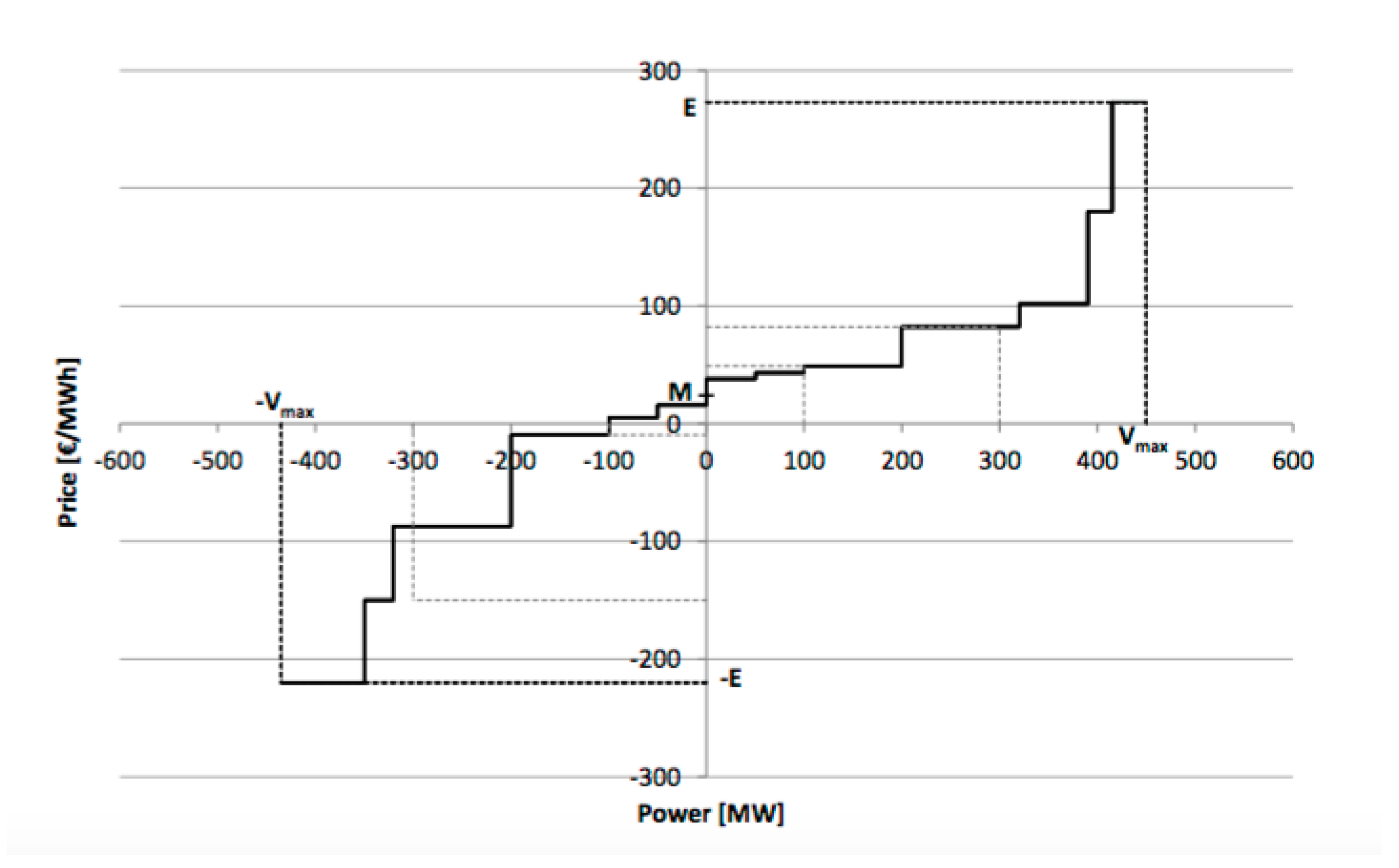
Despite the settled imbalance price being known only after closure of the reserve market, the current bidding ladder, as shown in Figure 1, as well as the procured reserve and regulating power that are provided by TenneT give an indication of the settlement prices. An update of these values is published every minute. The bidding ladder is made up of energy bids incrementally ordered for positive reserve power and decremented for negative reserve power. As is seen in Figure 1, the maximum upward and downward reserve capacity is depicted as E and −E, respectively, and is the maximum offered reserve volume. The mid-price M is the median between the lowest price bid for upward and the highest price bid for downward regulation [14]. If no regulating power is activated at a particular program time unit (PTU), then this mid-price Mis the imbalance price [15]. Using the published real-time price delta, BRPs can passively participate in the imbalance market by counteracting the current imbalance in the control area. In the Netherlands, the BRP received remuneration for this response if it contributes to the reduction of system imbalance.
As is the case in the day ahead market, it is assumed that the impact of the balancing power offered by the VPP has a negligible effect on the settling imbalance price. Therefore, historic prices are used in this simulation as the settling imbalance prices.
3.4. Machine Learning Model
Before an aggregator can offer flexibility for smart grid services, much like industrial size resource, the available flexible capacity (ramp up and down capabilities) must be known. Without this knowledge, the aggregator risks penalties due to not fulfilling offered resources and, even worse, creating grid instabilities due to generated imbalance. For aggregated flexibility, having detailed measurements to calculated this capacity is often not an option or too costly to install. Therefore, forecasting flexible capacity using aggregated data is an important step to enable aggregator participation in wholesale electricity markets.
It has been proven that black box machine learning techniques can accurately forecast the available flexibility of a homogeneous VPP as shown in [1]. Here, two supervised machine learning techniques were applied, linear regression and an artificial neural network (ANN). Both were applied with a black box approach, meaning only top level or aggregated information was known. Specifics of the virtual power plant such as device type, state of charge or nominal power were unknown to the prediction models. It was found that the ANN model significantly outperformed that of the linear regression model. Therefore, for this study, an ANN model will be implemented to investigate the accuracy when applied to a heterogeneous VPP.
An ANN predictive algorithm can be considered a black box because of its ability to approximate a function without knowledge or having insight into the structure itself. Here, we have used a supervised ANN approach, where the model uses a training set of recorded data to train a hidden layer of neurons to model a non-linear relation between the input and output data.
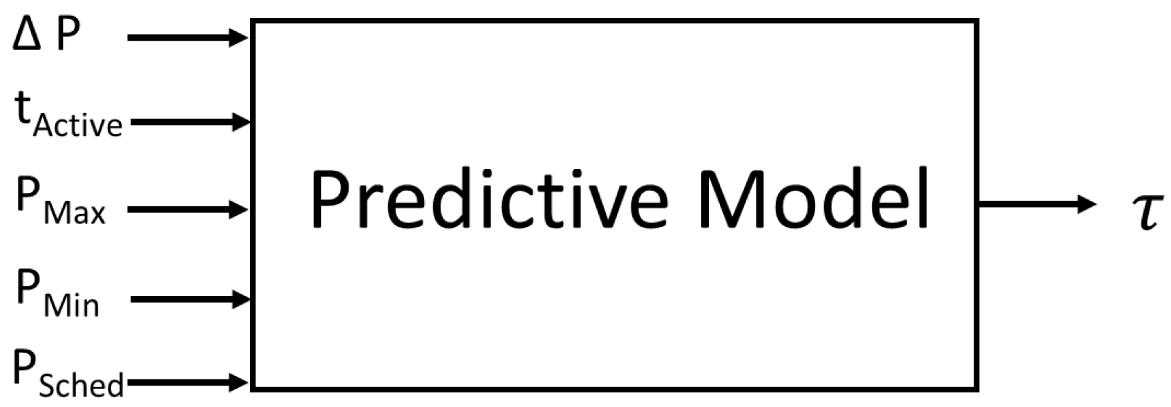
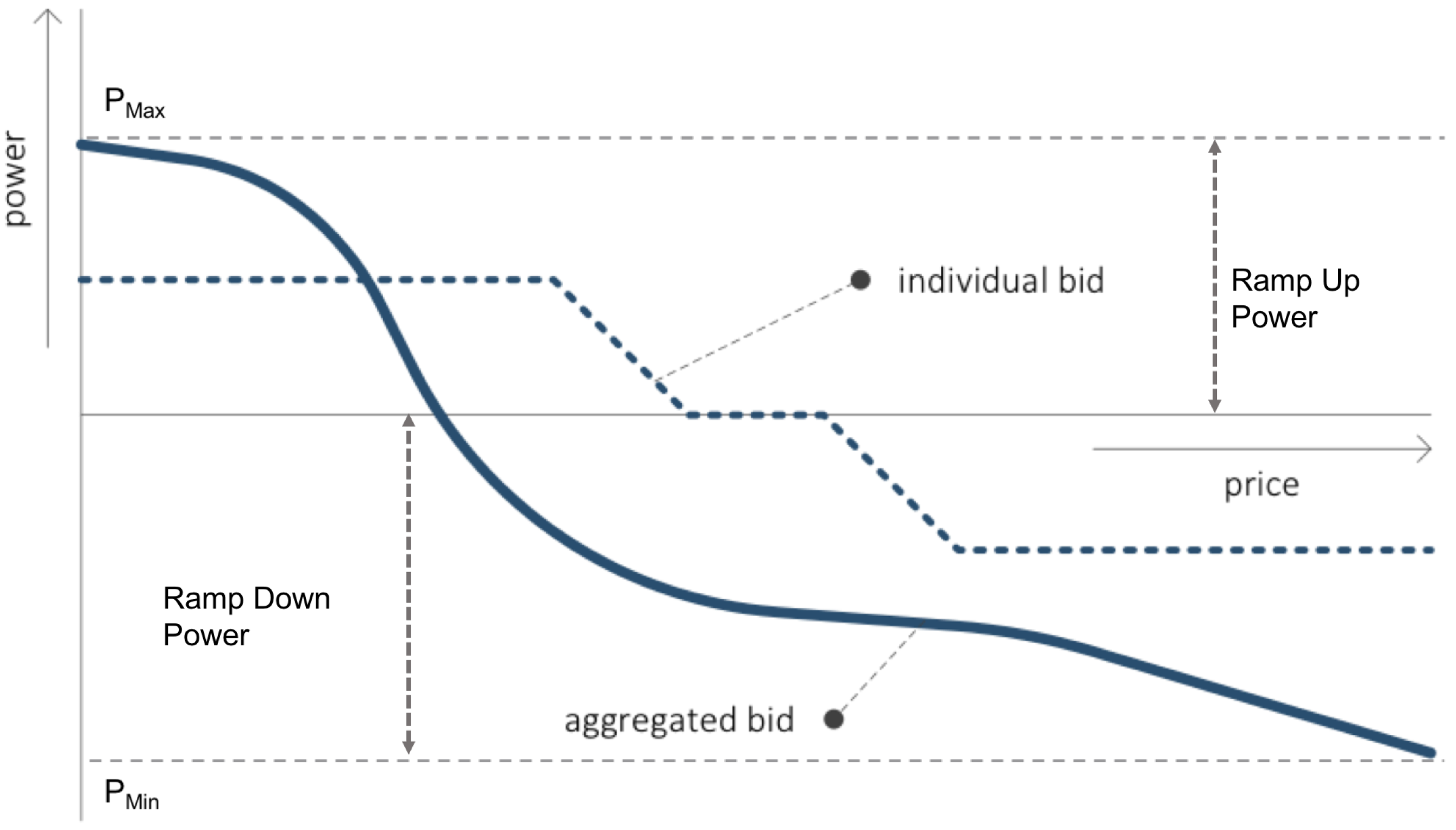
The ANN model implemented is a single hidden layer with a sigmoid transfer function as described in [1], which models the relationship between the input and the output data. For this model, as depicted in Figure 2, the input data are: ramp power (), which is the requested deviation power from the current day ahead scheduled power, scheduled activation time (), day ahead scheduled power at the time of activation () and maximum and minimum bid ( and ); with the output of the model being longevity (), i.e., the length of time the provided ramp power can be sustained. In the context of this study, ramp up power is the amount of power for which the VPP will increase its combined load from the scheduled day ahead profile and ramp down power the amount of power for which it will decrease or shed load. Further, from Figure 3, defines the maximum power that the VPP can increase its load at a given moment, and is the maximum it can shed load.
In Figure 3, an example individual bid for a device and the aggregated bid for PowerMatcher can be seen. These individual bids are near real time and event based to depict the priority of a device to produce or consume electricity. An aggregated bid is the summation of all valid bids sent by the individual devices in a VPP. To ensure all device-specific data are removed, only the top level, aggregated bid is used to forecast the real-time flexibility. Here, the maximum and minimum power ( and ) are retrieved as input to the forecasting model. This is the similar upper and lower bound power information that can also be retrieved from an offer to an electricity market from a resource owner. This defines boundaries for the amount of ramp up and down power the VPP can provide. Further, using this bid and the current price, the current total aggregated power of the VPP can be calculated.
The ramp capacity in both directions is then calculated by requesting a ramp power, which is one of the power steps in the aggregated bid and multiplying it by the forecasted longevity (). For a ramp down capacity, the requested ramp power sent into the model is negative as negative power represents a power supply.
4. Multi-Market Trade Implementation
To evaluate the economic impact of a forecasting model for wholesale market services, a trade strategy has been developed that can be implemented for all three cases: without forecasting of shiftable capacity (worst case), black box machine learned ramp up and down capacity and that with the perfect knowledge of VPP flexibility, as well as the wholesale market prices (best case). Using the same control strategy for all three cases allows for a fair comparison of the effectiveness of the black box machine learning model to the best case, full knowledge scenario and the worst case, no capacity knowledge.
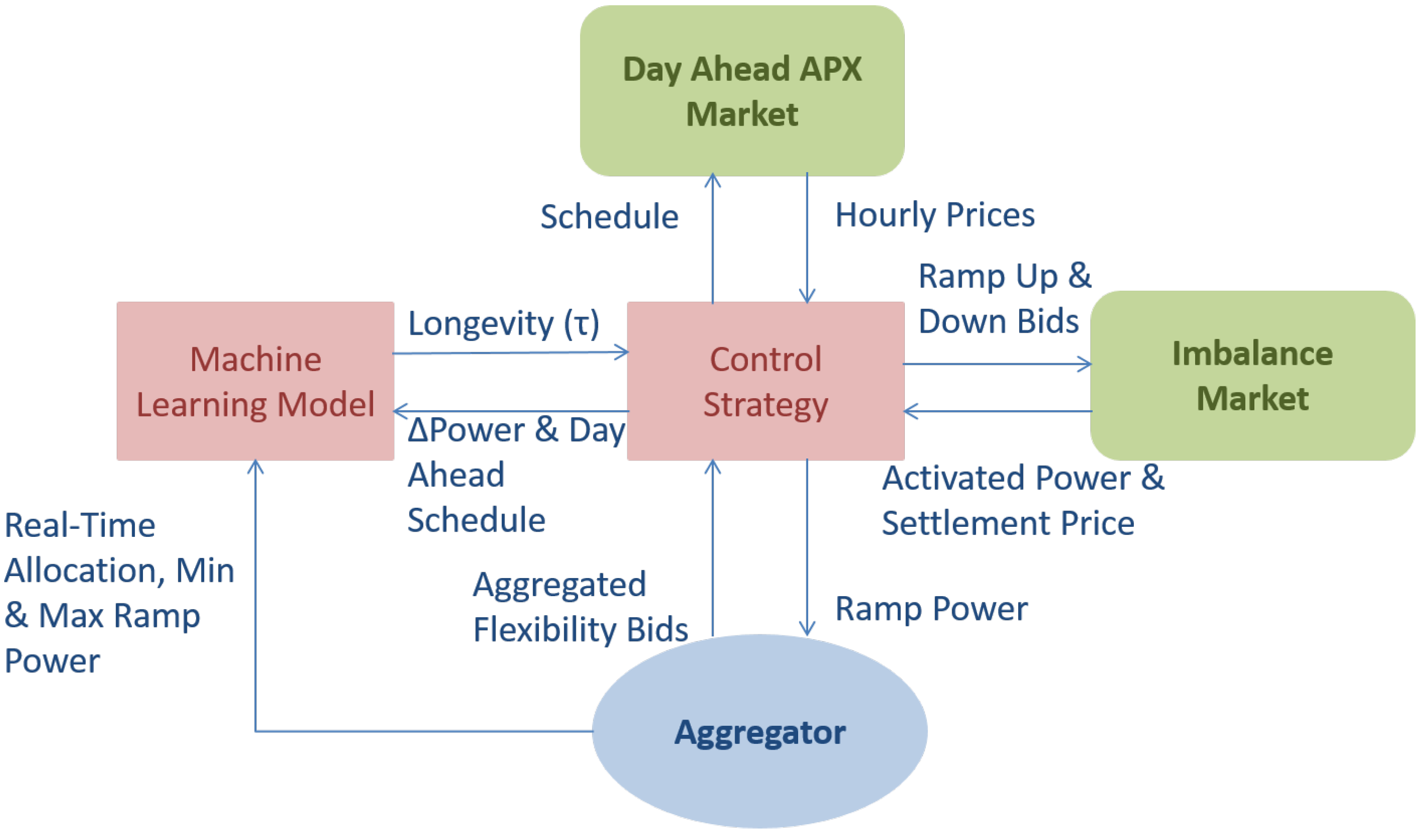
Figure 4 presents an overview of the information exchange between the wholesale markets and the aggregator. Here, it can be seen that two wholesale markets are participated in, the DAM, which results in a daily schedule, and the imbalance market. Each of the three cases use a pre-determined day ahead profile, which was created to minimize the cost of electricity purchased on the current day ahead market. The generations of this profile are defined in Section 5. Using this, the trade strategy module is fed, in real time, the aggregated bid to determine the ramp power sent to the machine leaning module described in Section 3.4.
The flexible ramp up and down capacity estimated by the machine learning module and the day ahead profile, generated daily from the APX DAM market, are used to calculate the remaining flexibility, which is traded on the imbalance markets. For the first two approaches, as is currently the case in the Netherlands, no forecast and forecasted flexibility, the imbalance prices are only known after settlement. Therefore, their lower bound, willingness to sell, and upper bound, willingness to buy power, is based on historic prices, in this case the previous day’s imbalance price spread. For the perfect knowledge approach, to provide a best case scenario, the future imbalance price spread for the current day is known before trading.
4.1. Assumptions and Constraints
The trading strategy assumptions defined for this study are defined below:
- The imbalance market is a dual pricing system for short and long offers like that of the Dutch balancing market.
- The imbalance market will operate on a 15-min time slot.
- The administration fee, , will be neglected for imbalances.
- The aggregator is able to freely participate in the market.
The following constraints defined below are implemented to ensure that the aggregator is profitable, as well as to guarantee limited negative impact on the stability of the network:
- The VPP will ramp up, increase consumption or reduce production, only for negative prices.
- The ramp down marginal cost must be higher than the current day ahead APX price.
- The VPP must consider future, day ahead schedule requirements in trading.
- The VPP cannot offer ramp power outside the bounds of the aggregated bid.
4.2. Trading Strategy
The trading strategy implemented tried to find a balance between maintaining future and current day ahead scheduled obligations and offering flexibility on the imbalance market. The following logic is used for every 15-min time period. Firstly, the total available ramp up, , and down energy capacity, , are calculated. The calculations are different for each of the three approaches:
(1) For the no forecasting approach, the ramp up capacity is estimated using Equation (1):
with being the current maximum ramp power of the VPP aggregated bid as seen in Figure 3, the current day ahead scheduled power and the time interval of the imbalance market, 0.25 h (15 min).
Similarly, the ramp down capacity in watt hours (Wh) is estimated using Equation (2):
with being the current minimum ramp power of the VPP aggregated bid as seen in Figure 3.
(2) The forecasting capacity approach applied the ANN model described in Section 6.2 to forecast the for a set of ramp powers, , , , ⋯ , and ramp down powers, , , , for values that are greater than zero. By multiplying with its affiliated ramp power and averaging the calculated ramp up capacities and down capacities, available ramp up and down is estimated. In the case that the ramp up or down power is less than or equal to zero, the associated is set to zero, and the VPP is unavailable for imbalance trade.
(3) The perfect knowledge implementation calculated the and by having each device submit its current ramp up and down capacity in combination with its PowerMatcher bid and, at the top, aggregating the capacities for both directions. Each device calculated its available capacity with perfect user behavior foresight (for example, heat demand).
The future day ahead obligations are secured by removing the ramp up and down energy needed to fulfill the next hour’s scheduled day ahead profile. This required energy is calculated in Equations (3) and (4) with being the current total allocation of the VPP:
and:
Using , the remaining flexible energy available to offer on the imbalance market is determined:
and:
As the first two approaches do not have perfect foresight of the imbalance prices, the maximum and minimum settlement imbalance prices from the previous day, and , are used to determine their willingness to buy and sell flexibility. The perfect knowledge implementation based its price bounds on the imbalances prices of the same day being traded. Therefore, in Equations (7)–(10), the parameters and can be replaced with and for the perfect knowledge scenario. This is done to provide an upper bound to compare the performance of the forecasting approach.
The expected minimum and maximum price range defined and , the maximum of the previous day’s , were used to calculate the minimum cost at which the VPP will buy or sell energy:
and:
Note: in the instances where from Equation (8) was greater than zero, the last negative price was applied.
For each time period, or quarter, two unique bids were offered on the imbalanced market. The bids were comprised of an array of power between the range of zero and and each associated willingness to buy or sell in €/MWh. is / , for ramp up and / , for the ramp down balancing bid. Finally, and are calculated with Equations (9) and (10) where →, the power steps in the offered bids:
and:
It was assumed that if the imbalance price falls within the price range of the aggregator’s offered bid, it will automatically be selected. Therefore, the VPP increased or decreased its consumption according to the offer placed for that quarter.
5. Simulation Scenario
The residential VPP modeled for this study consists of 1000 unique households. This is a scaled version of an intelligently controlled pilot called PowerMatching City located in Hoogkerk, The Netherlands [17]. Further, the VPP consists of controllable space and domestic hot water heating devices, white goods (washing machines, dish washers and dryers) as well as cold storage (refrigerators and freezer). Additionally, every home is coupled with a unique space heating, domestic hot water and base non-flexible electricity demand profile. Each profile is created with a resolution of one minute using a validated software tool, TNO’s energy pattern generator [12], which can generate profiles for five residential home building types. All households have an intelligently-controlled heating device, 800 heat pumps and 200 micro-CHPs, which is coupled to a 110-L space heating buffer and 90-L domestic hot water buffer. The division of white goods in each household is presented in Table 2 and mirrors the results found in a study done in the Netherlands [18]. The nominal power of the washing machine, dishwasher and dryer is the maximum power over all the cycle profiles defined in the model.
Similar to the implementation in PowerMatching City, each home has a small photovoltaic (PV) panel. For this, real PV measurements are utilized and scaled to match that of 1000 households (1240 kW nominal electric power). Finally, the amount of offshore and onshore wind in the simulations is based on the WLO-SE(Welfare and Living Environment) scenarios on energy supply and demand with a time horizon up to 2040 [19], which has been scaled down to reflect that used in a residential VPP of 1000 households. Additionally, the residential demand for all the households is set to be 130 PJ. In [19], the expected total electricity demand for the Netherlands is 582 PJ; of that, the residential demand is 130 PJ. For these simulations, this value has been scaled from 8.6 million to 1000 households.
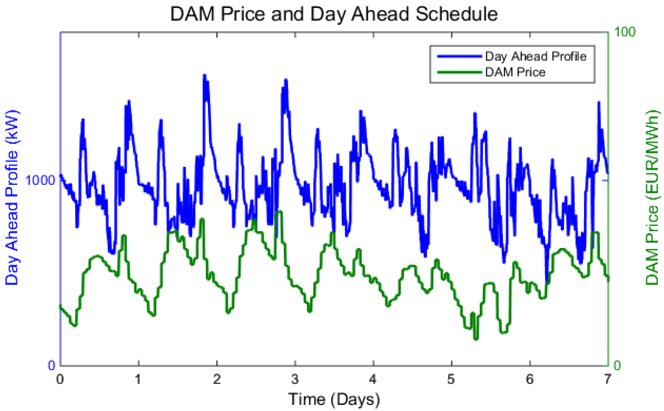
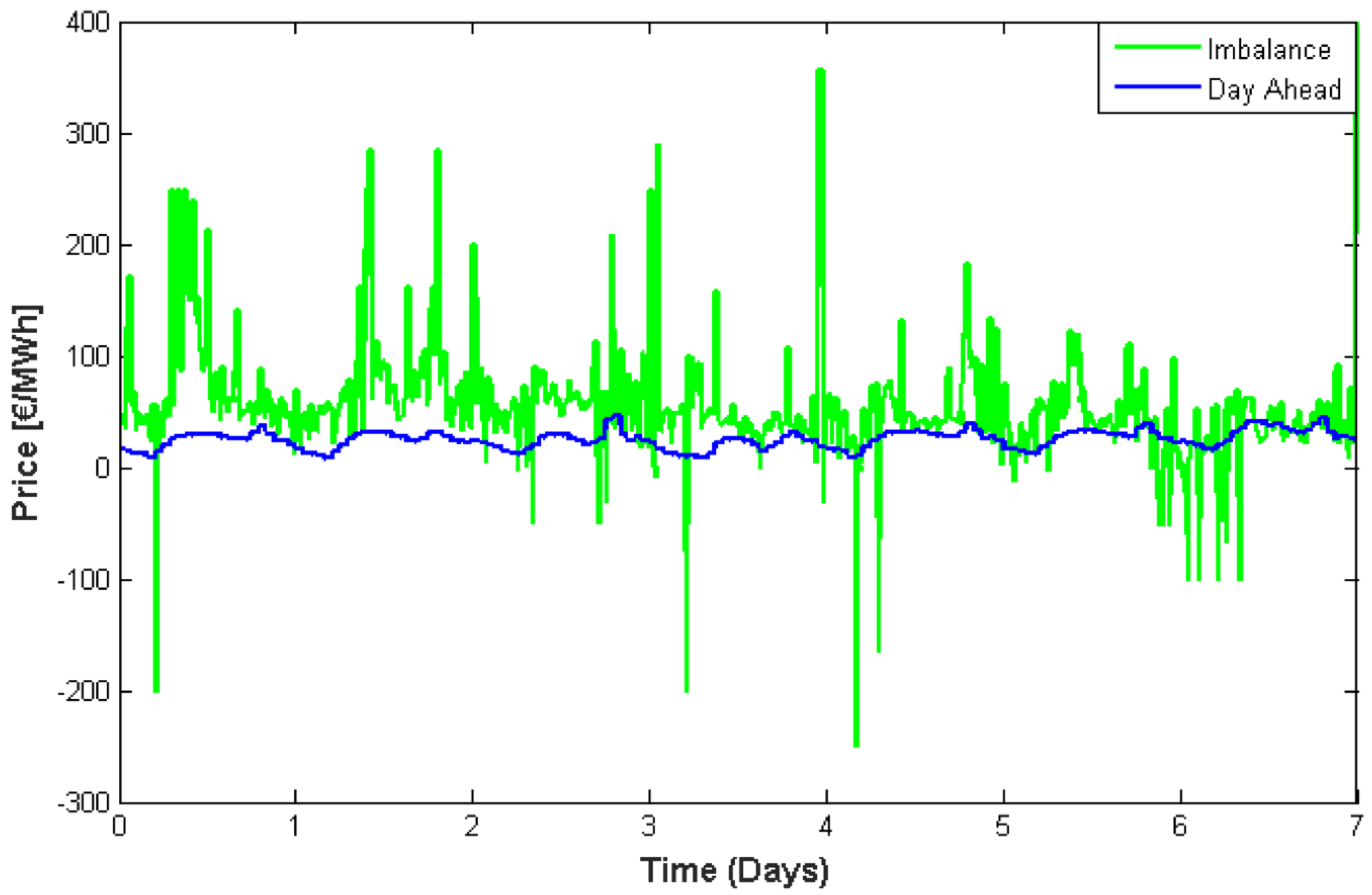
All three of the trading approaches used historic day ahead prices, APX, and TSO imbalance price and volumes, TenneT (Dutch TSO), to simulate the month of March in 2016. The day ahead schedule was generated by steering the PowerMatcher-controlled VPP with the current day ahead prices. The resulting aggregated power profile of the total VPP was then averaged to create a 15-min resolution day ahead schedule. Figure 5 presents a comparison of the DAM prices and the generated optimal day ahead profile. The price settlement for the imbalance market is performed every 15 min. As was stated in Section 4, the imbalance prices are known to the aggregator after settlement for the first two trade strategies, no forecasting and black box capacity forecasting. For the perfect knowledge scenario, the willingness to pay of the aggregated flexibility is based on current day imbalance prices, which are given to the aggregator before trading. If the trade strategy results in a reduction of system imbalance (the system is short and the aggregator long), a profit is seen for the aggregator. Inversely, if an imbalance is generated, the aggregator has a financial cost. Figure 6 shows a comparison of the imbalance and day ahead price profiles used for this simulation.
6. Validation of Models
In Section 4, the trade strategy to participate in the imbalance market is described. The trade strategy was implemented for three cases. The first case, no forecasting, does not have knowledge of the available ramp up and down flexible energy. Instead, the capacity was estimated using the real-time maximum and minimum power taken from the aggregated bid. The second case applies a supervised machine learning technique to predict the available flexible energy. This will be validated by performing a sensitivity analysis of the forecasting model’s performance based for various compositions of heterogeneous VPPs. The forecasting model will then be validated for the specific heterogeneous VPP defined in Section 5. The third case, perfect knowledge, applied a bottom-up approach to calculate the flexible ramp up and down capacity, as well as used perfect imbalance price foresight to assign cost to the offered flexibility.
The following subsections will describe the modifications to the trade strategy for each case, as well as data required and the validation of the machine learning model.
6.1. No Forecasting
Using marginal cost calculations for the offered balancing power and trading strategy described in Section 4, minor modifications were made to accommodate the flexible capacity being unknown. To begin, it is assumed that the VPP is capable of maintaining the current maximum ramp up, , and down power, , for the entire imbalance quarter. The available ramp up and down capacity is calculated by multiplying the maximum ramp up and down power by 0.25 or 15 min. This is assuming that is greater than and is less than . To take into account the future day ahead schedule, the VPP’s current conditions are assessed, maximum and minimum power of the aggregated bid, to determine if it is capable of achieving the future scheduled power. In other words, it evaluates if the future day ahead scheduled power for the next hour lies within the current upper and lower power limitations of the aggregated bid. If it does not, the VPP will not trade on the imbalance market for that quarter. To calculate the upper and lower values for the value assignment of the flexibility, the minimum and maximum values of the imbalance prices from the previous day are used.
6.2. Machine Learned Capacity
The black box machine learning model had only previously been applied to a homogeneous VPP of heat pumps [1]. However, especially in the residential sector, it is more common to couple a diverse set of mixed types of flexible devices. The robustness of the model was first researched by applying it to heterogeneous VPPs where the three device types’ penetrations were varied. This analysis provided confidence in the versatility of the model for all types of residential VPPs and guaranteed accurate offers of residential VPP flexibility for market operation.
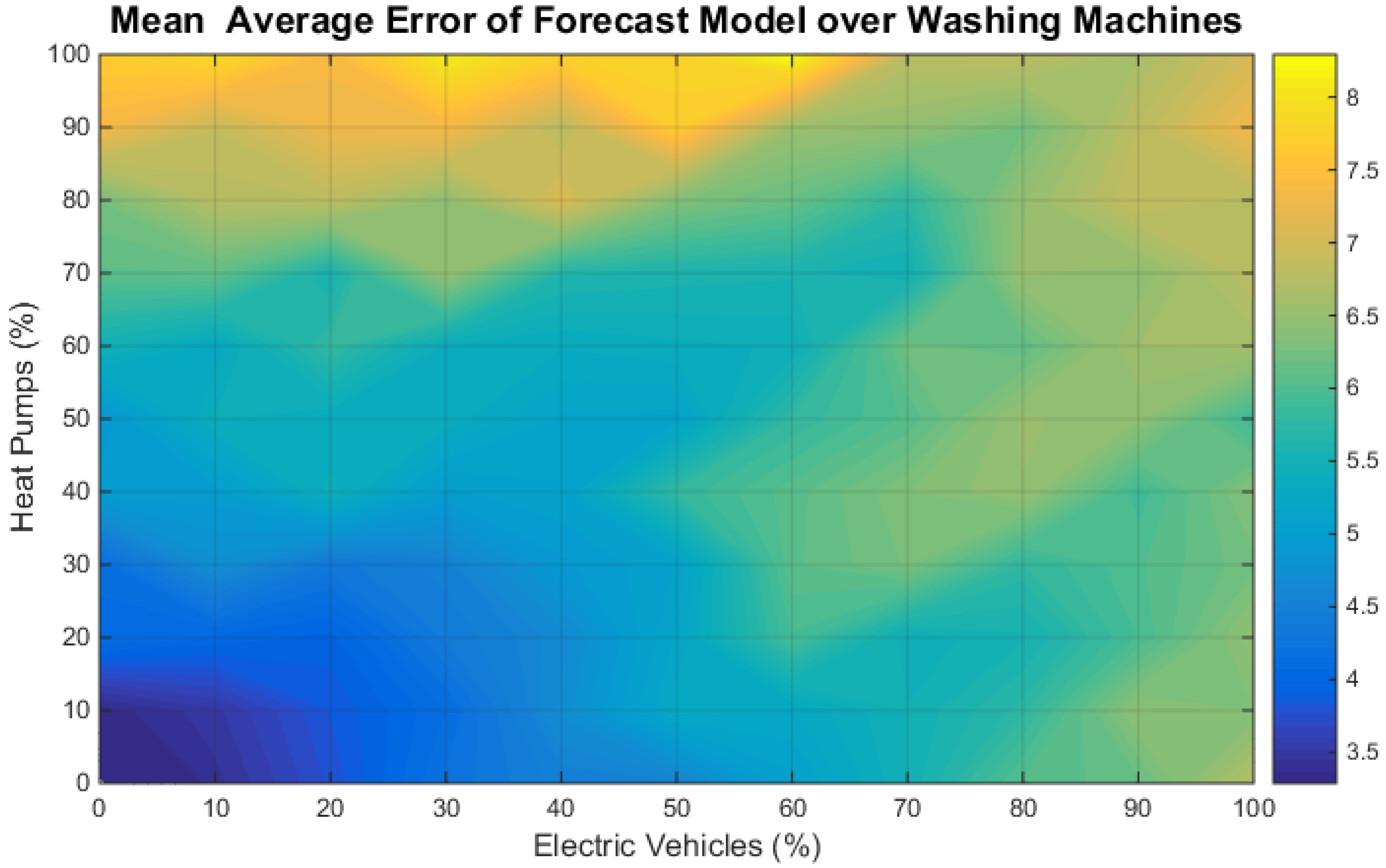
The three most common and largest types of flexible devices found in a household are the time-shifter, thermal storage and electric storage [8]. Therefore, the sensitivity of the ANN model when applied to a varied set of VPP make-ups consisting of electric vehicles (EVs), washing machines and heat pumps is investigated. Each device model has its own individual behavioral properties such as heat demand and drive patterns. The number of households in the heterogeneous cluster was fixed to 1000 households. Based on 1000 households, the penetration of each device type is varied between 0:100:1000 per VPP results in a set of 1331 distinct VPPs. For each VPP, the ANN model was trained with 200 sets of ramp up and down power deviation data and validated with 100. The mean average error (MAE) for each validation set of all VPP variations was calculated.
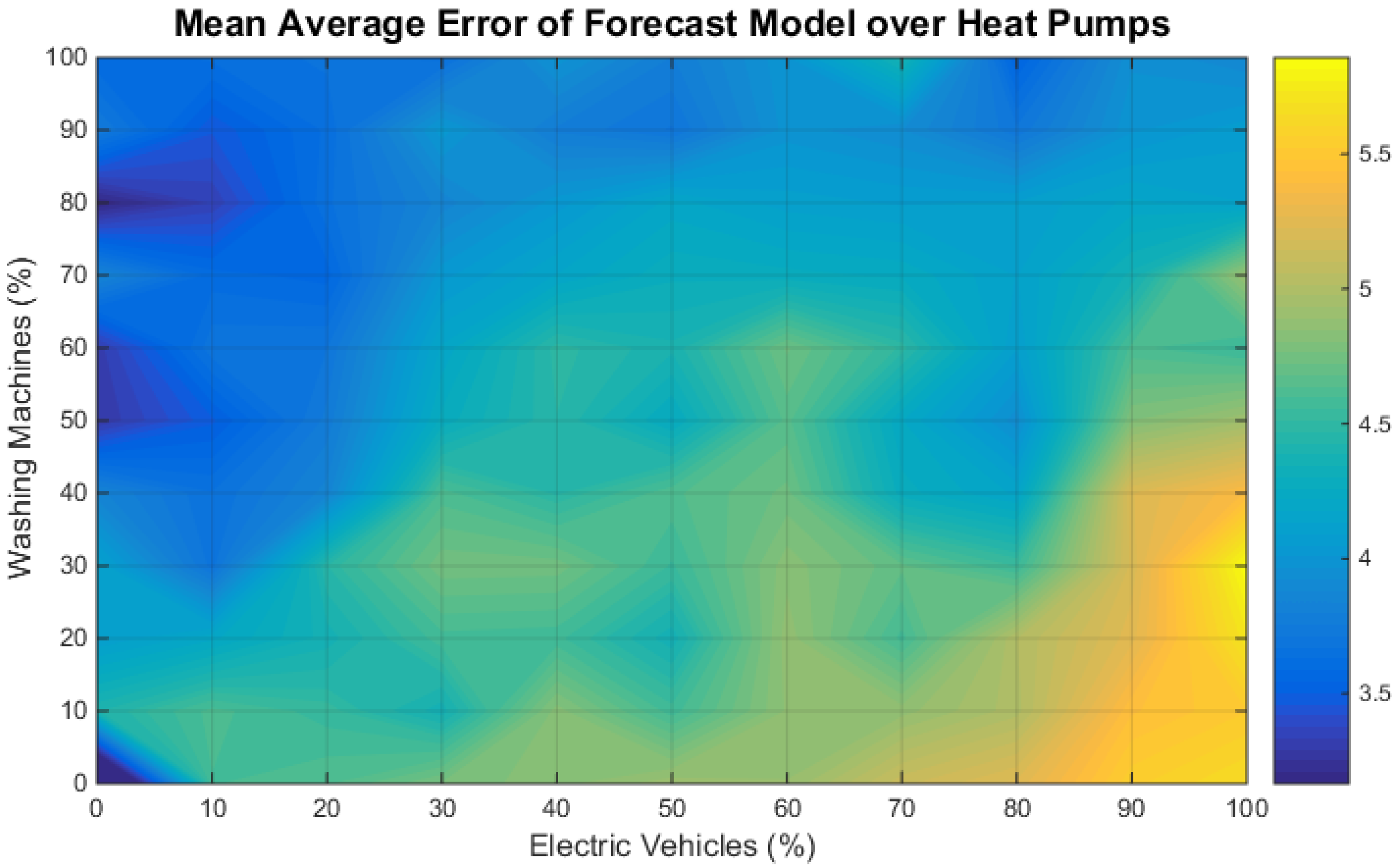
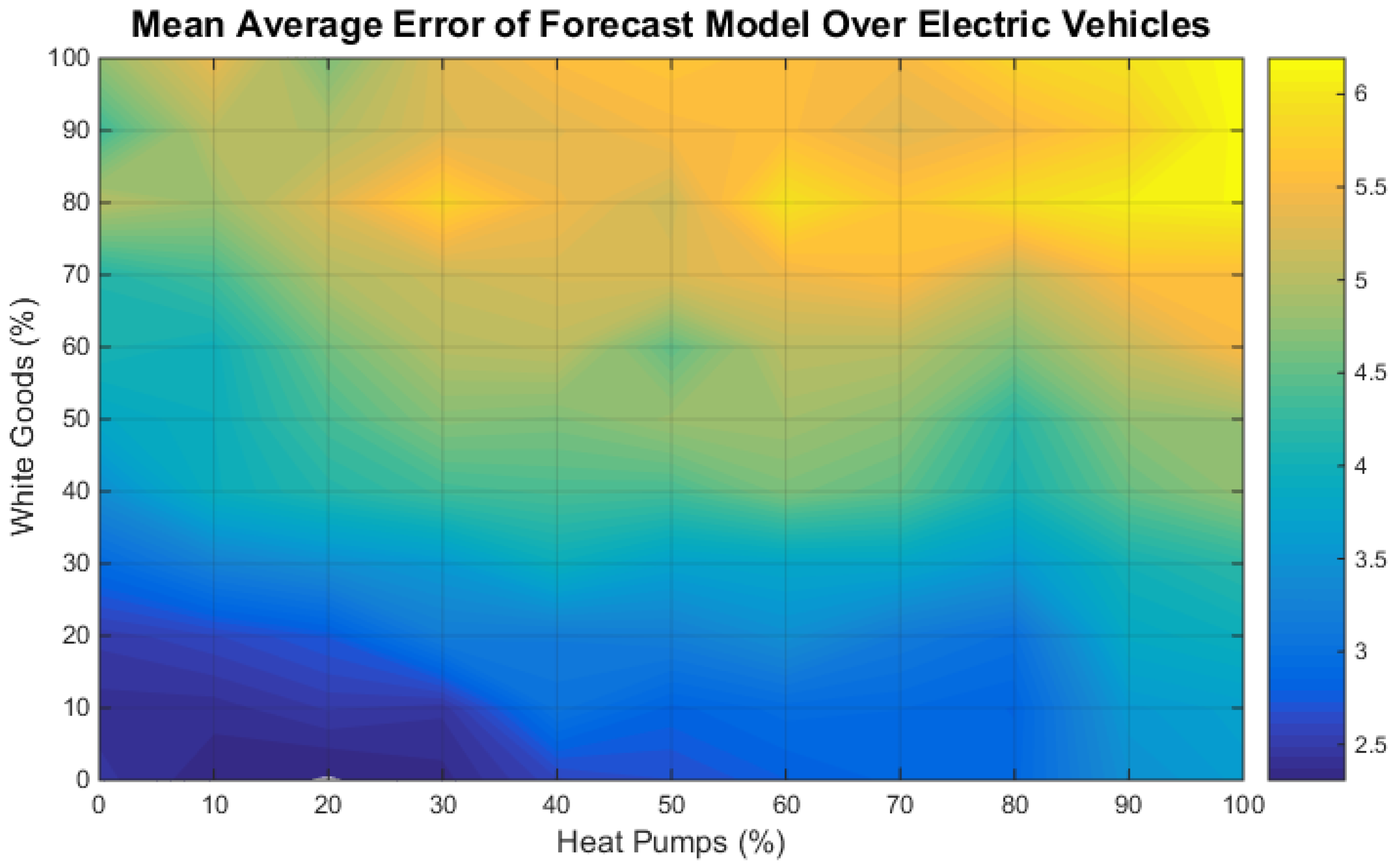
Overall, the maximum MAE for all types of VPP seen was 9.8%. This in itself proves the versatility of the ANN model for all types of residential VPPs and the ability to maintain a high accuracy despite the small training set. From here, it can be seen that white goods have a much lower impact on error than those of electric vehicles and heat pumps. To investigate further, the mean of the MAE is fixed for one device and plotted with the other two varying. To investigate the impact of an individual device type on the error of the ANN model, the MAE was averaged over one device type. Figure 7, Figure 8 and Figure 9 present the MAE when the VPP error is averaged over all penetrations of heat pumps, EVs and washing machines. These figures depict that a heat map is presented for each device type, where the lower to higher error is represented with a respective color range of blue to yellow. Overall, the maximum error seen when averaging over heat pumps, EVs and washing machines was 5.8%, 6.3% and 8.4%, respectively. Overall, for all types of heterogeneous VPPs, the mean percent error is under 10%, which proves the versatility of this forecasting model for any type of residential VPP. The ANN model was then trained and validated using the cluster scenario described in Section 5. As was stated previously, the model applied uses a black box approach and has been validated with a homogeneous cluster of heat pumps in [1]. The heterogeneous VPP represented 1000 households, each containing flexible devices, which consisted of a heating device, white goods and cold storage. The ramp up and down powers used in the ANN model are deviations from the defined day ahead schedule. The output of the model is the longevity , the amount of time the VPP can hold a ramp power. Using a series of ramp powers and their associated longevity, the flexible capacity for ramping up and down can be calculated.
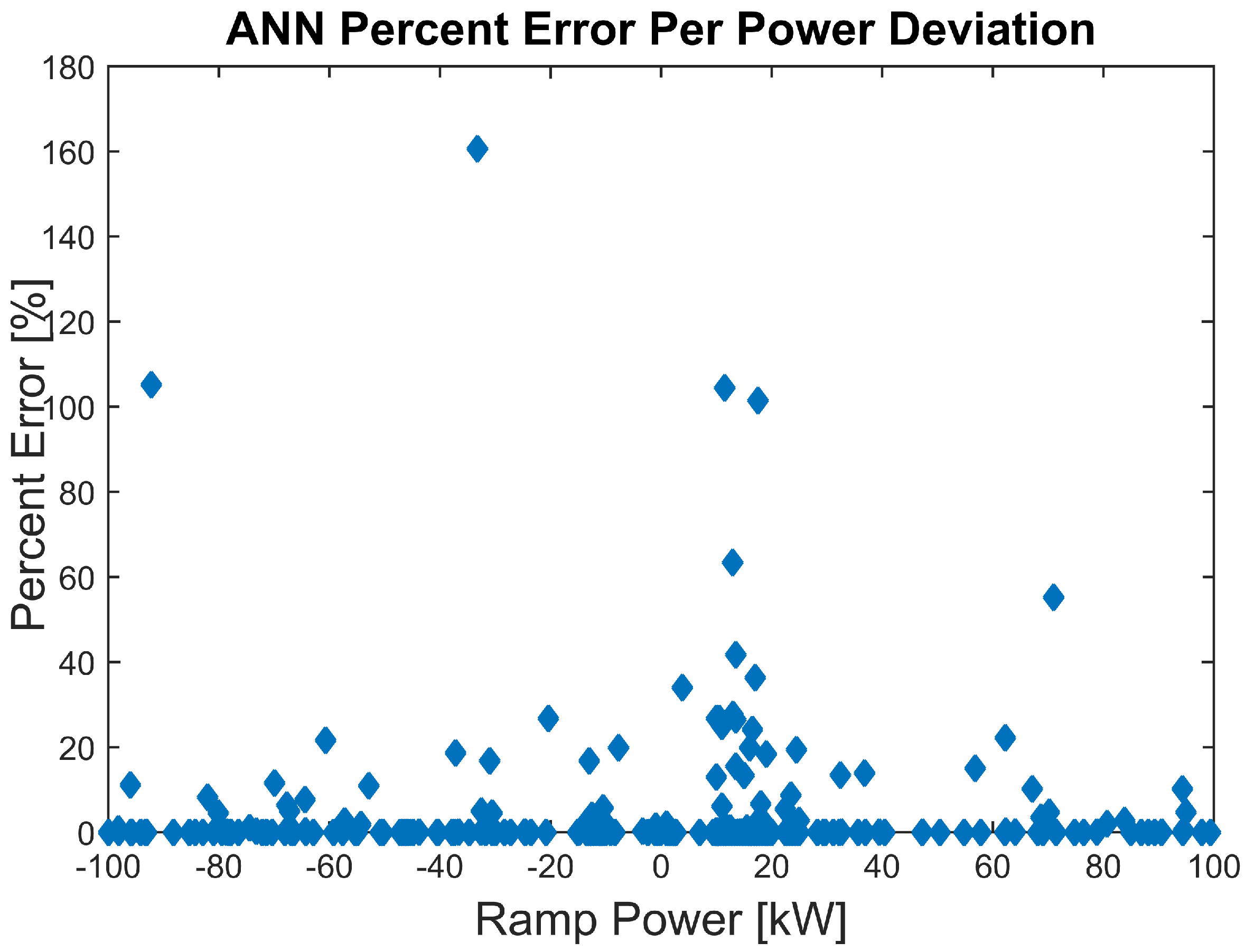
The dataset used to train and validate the ANN model was comprised of various ramp powers ranging from −100 kW–100 kW. The hour at which the ramp power was requested was also varied in time for different hours of the day. The dataset consisted of 2000 unique observations, 1500 rows for supervised training of the model and 500 for validation.
As presented in Figure 2, to validate the model, once training is completed, the supervised ANN model is fed the day ahead profile of the VPP, as well as the desired ramp power and ramp time to forecast its associated longevity . These values were compared with the actual response to evaluate the performance.
In Figure 10, the forecasting errors for the validation set can be seen. Despite a few outliers, the overall average error was 4.28%. The performance is comparable to that seen in [1] where the average error was found to be slightly lower, 2.3%. This is due to [1] forecasting a homogeneous VPP of heat pumps compared to the much more complex heterogeneous VPP used in this experiment. Further, it can be seen that there is no correlation between error and ramp power. Using and ramp power, the capacity can be estimated. When comparing the estimated capacity versus the actual capacity for each validation set, the average error was seen to be 7.41%.
As is described in Section 4, this validated and trained ANN model was then implemented to forecast the run-time available ramp up and down flexibility. Like the no forecast case, the value assignment of flexible capacity uses the highest and lowest imbalance prices from the previous day.
6.3. Perfect Knowledge
The perfect knowledge case uses perfect price and available flexible capacity to participate in the imbalance market. For this approach, each flexible device calculates its available ramp up and down flexible capacity every 15 min based on its current electricity load requirements. The total available ramp up and ramp down capacity is calculated by aggregating the values of each device. Additionally, the ramp up and down capacity needed to meet the future electricity requirements from the inflexible load profiles is included in this calculation.
Unlike the no forecast and forecasting capacity case, the perfect knowledge case has access to the current day’s imbalance prices before trading. While this is not possible in the real world, it provides an upper bound to evaluate the performance of trading when forecasting the available flexible capacity.
7. Results
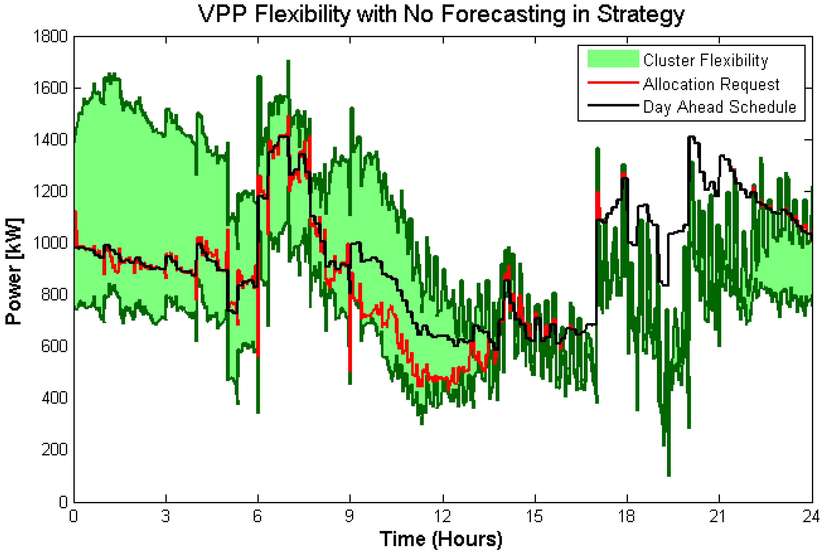
The multi-market trade strategy described in Section 4 was applied to the three approaches and run for the month of March. The VPP’s available ramp up and down flexible capacity for a typical day in the “no forecast” case is shown in Figure 11. Here, as a result of having no knowledge of the shiftable flexibility, fast degradation of the flexible capacity is seen. Therefore, at times, insufficient flexibility is remaining to meet the future day ahead schedule obligations after trading on the imbalance market, resulting in a portfolio imbalance.
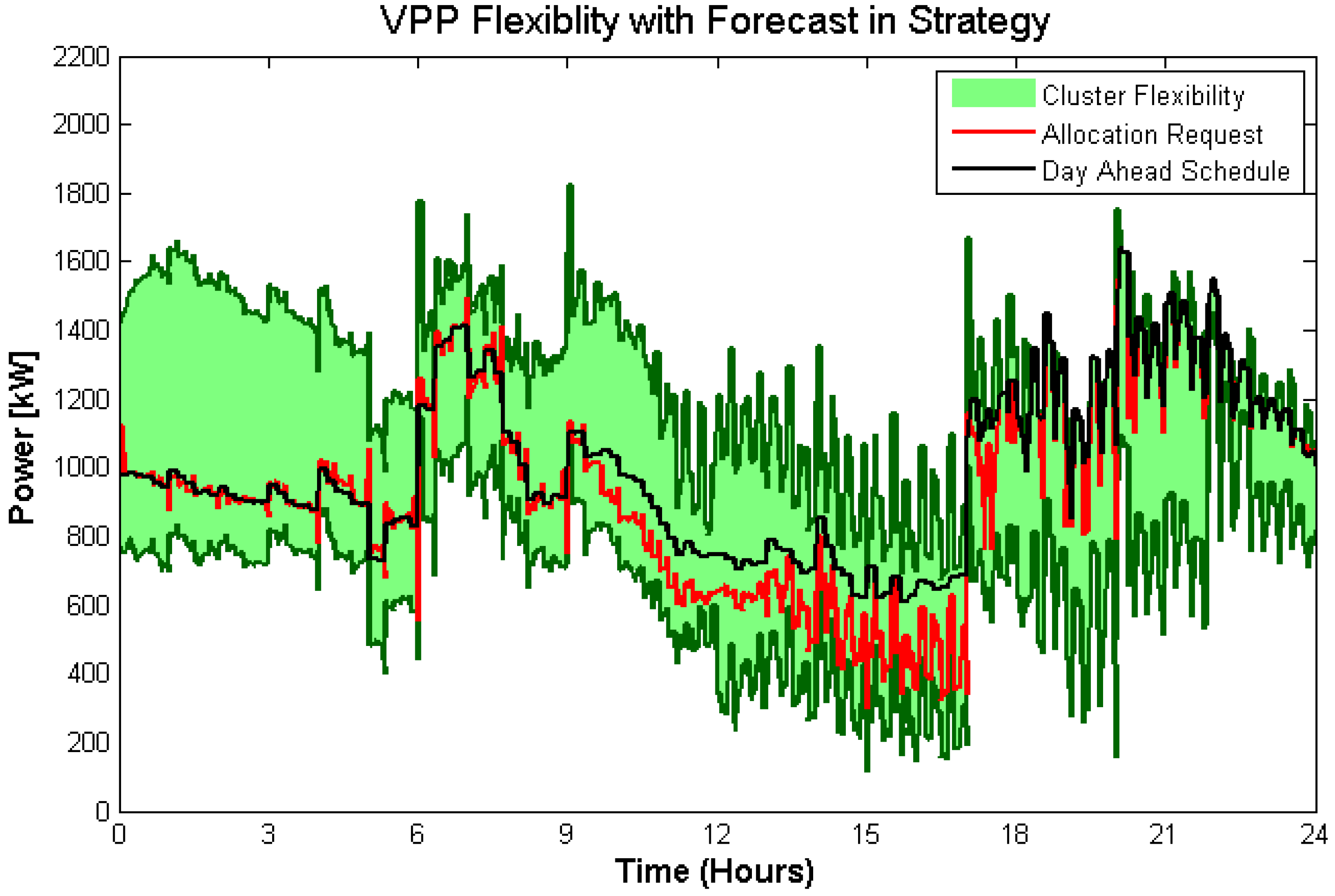
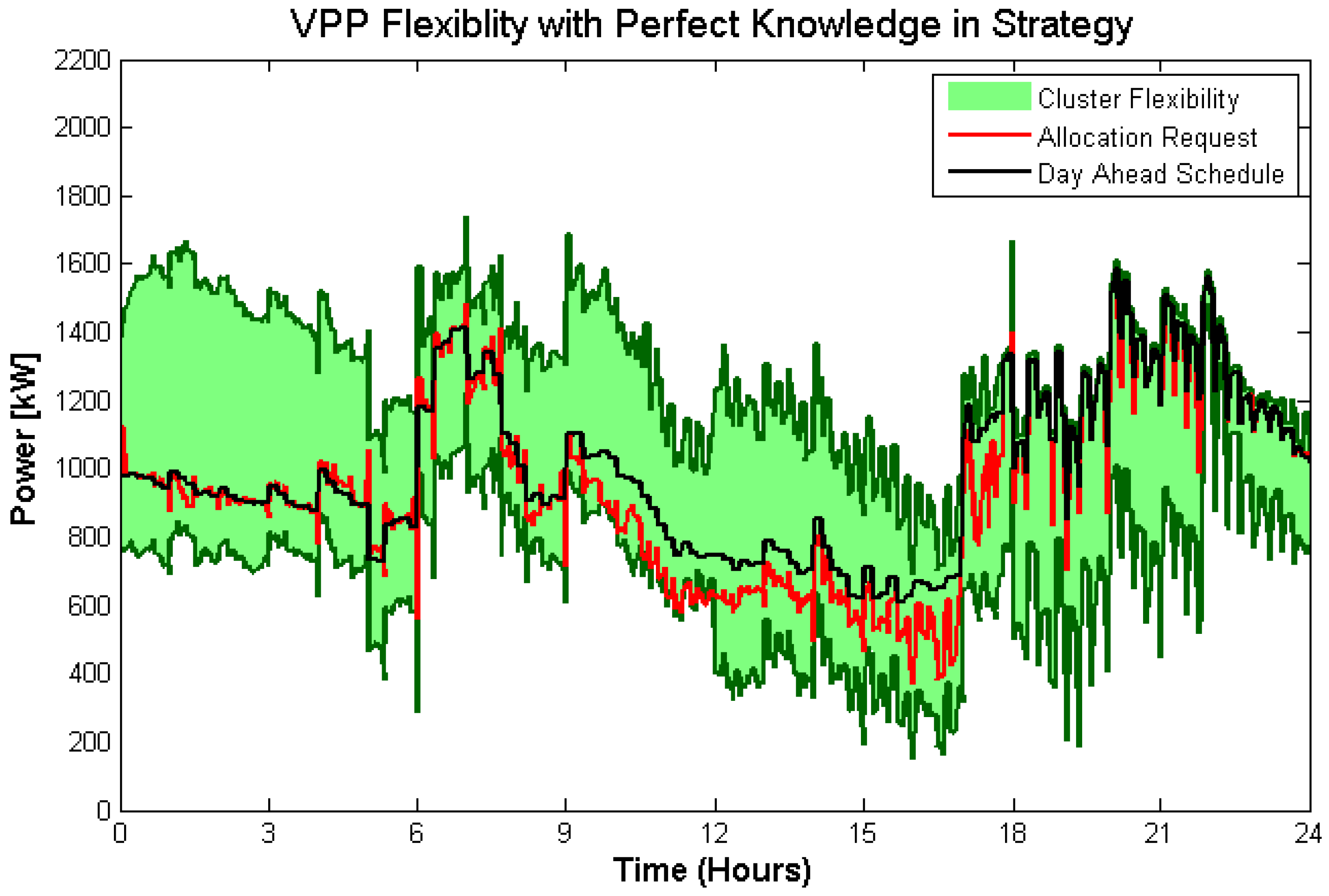
Figure 12 presents the same day when applying the forecasted flexibility to the trade strategy. Figure 13 shows that sufficient flexibility is provisioned to significantly reduce generated imbalance from over-trading. For the perfect knowledge case, the residential VPP did not generate unwanted imbalance.
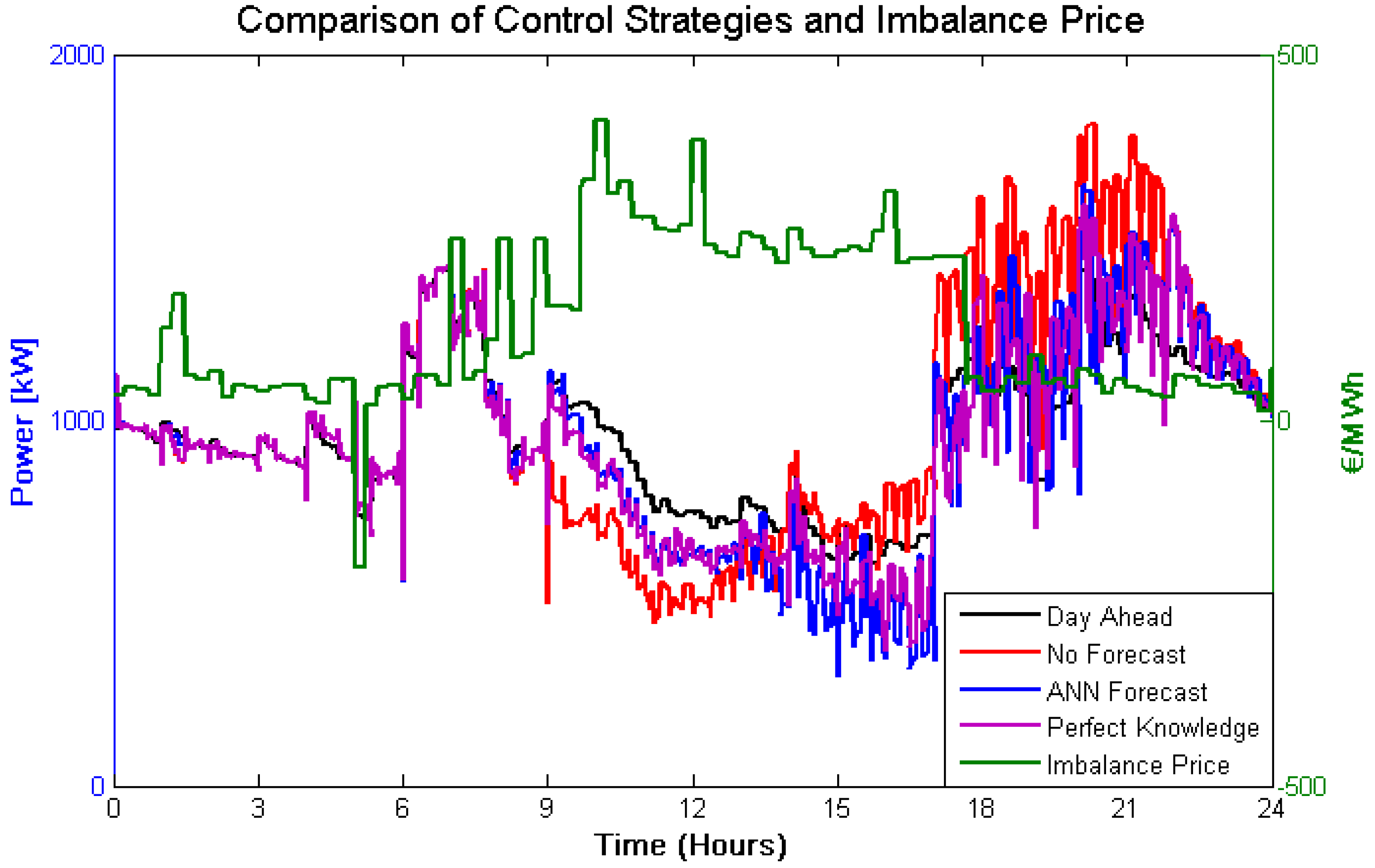
The resulting allocated aggregated power per trading case versus the settled imbalance price can be seen in Figure 14. At Hours 9–12, it can be observed that the no forecast case offers the most ramp down flexible capacity due to the high imbalance prices. However, at Hours 18–24, an imbalance is generated due to insufficient reserve flexibility for day ahead obligations. The forecasted capacity and perfect knowledge cases are able to maintain the day ahead schedule in the evening, eliminating a potential generated imbalance, due to trading less flexibly in Hours 9–12.
As all three cases used the same day ahead schedule and DAM prices, they all had the same DAM costs. The DAM cost for buying power for a 1000 VPP for one month was found to be €16,773. A detailed economic performance assessment for each case can be seen in Table 3. In the table, the cost value represents the cost as a result of generating imbalance for each case. Based on these values, it can be concluded that the case using the black box forecasting approach results in a reduction of imbalance cost by 82%. This is further reduced in the perfect knowledge case to 86%. Further, revenue generated as a result of trading on the imbalance market was notably increased for both the forecasted and perfect knowledge cases. Additionally, if the no forecast and perfect knowledge cases represent the upper and lower potential trading profit when offering this VPP’s flexibility on the imbalance market, the black box approach is able to reach 89% of the potential.
The potential profit from trading on the imbalance prices is not only determined by the available flexibility capacity, but also the settled imbalance prices. The no forecast and machine learned capacity cases used the previous day’s maximum and minimum imbalance prices to determine the upper and lower willingness to buy and sell energy. With the exception of a few days, the day to day minimum and maximum imbalance prices were comparable. On these days, due to a sharp change in outdoor temperature, the available flexible capacity was limited for trading. This decreased the impact, which could have been seen when comparing to the perfect knowledge trading case.
Finally, in this trading strategy, the calculated available flexibility capacity was not included in the calculation of the day ahead schedule. Further cost reductions could be seen if the ramp up and down flexibility is incorporated in this optimization. For example, the ramp down flexibility capacity could be increased by purchasing more energy at moments when the day ahead price is low and the imbalance is typically high.
8. Conclusions
In this study, an evaluation of a black box machine learning model, which forecasts shiftable capacity of aggregated flexibility in a VPP, when applied to a simple predictive control strategy for multi-market participation is presented. This was achieved by comparing the economic gains and losses to the performance of a perfect knowledge and no forecasted scenario to provide the best case and worst case for the performance assessment. It was shown that when applying a black box machine learning model, ANN, the flexibility capacity of most types of heterogeneous clusters can be determined with an error of under 10%, which proves that it performs at a high accuracy of >90. This type of approach allows the flexible capacity to be accurately predicted using only top level aggregated VPP data and ensures end user-specific information is protected. Further, the availability of this information can lower the risk of imbalance generated and, thus, costs when offering VPP flexibility for smart grid services. This was proven when applying the forecasted ramp up and down capacity of a residential VPP to a multi-market trade strategy. It was seen that 89% of the potential profit, the profit found from the perfect foresight approach, was realized without jeopardizing the stability of the network. As a result, the overall monthly cost to power a 1000-household VPP was lowered by 20%. Therefore, characterization of VPP flexibility is vital to limit risk when offering smart grid services. The available capacity can be accurately forecasted when applying machine learning techniques without the use of lower level device-specific information. Including this information in a trading strategy of an aggregator improves the performance overall when participating in wholesale electricity markets.
9. Next Steps
Up to now, the machine learning model has been tested using only one demand response algorithm. Next steps are applying the same control strategies using different demand response algorithms. This will also use machine learning to forecast not only the flexible capacity, but also recharge characteristics, as well as the drop out behavior of VPPs. This will be done with multiple aggregators simulated with hardware in the loop from two smart energy system labs: TNO’s HESI Facility in Groningen and EnergyVille in partnership with KU Leuven. Finally, investigation into incorporating machine learned capacity into DAM market trading to further lower overall costs will be done.
Acknowledgments
The authors would like to thank Anna Kosek and Bonna Newman for their valuable input in this work.
Author Contributions
Pamela MacDougall is the main author and designed and implemented the simulation. Bob Ran helped with the simulation. All authors contributed to the analysis and writing of the paper.
Conflicts of Interest
The authors declare no conflicts of interest.
Abbreviations
| ΔP | Requested ramp up or down power deviation compared to the day ahead scheduled power in W. |
| Longevity, amount of time in minutes a power deviation from the day ahead schedule can be held. | |
| Total available ramp up or down energy capacity in Wh. | |
| Ramp up or down energy capacity that is available for imbalance trading in Wh. | |
| Ramp up or down energy capacity that is required to meet future day ahead schedule in Wh. | |
| Activation time for in the hour of the day. | |
| Current ramp up or down power that is available for imbalance trading in W. | |
| Day ahead scheduled power at time of activation in W. | |
| Current total allocation of the virtual power plant in W. | |
| Maximum power of aggregated bid in W. | |
| Minimum power of aggregated bid in W. | |
| Time interval of the imbalance market in minutes. | |
| Minimum cost for ramp up or down services in €/MWh. | |
| Day ahead market price at time of imbalance trading in €/MWh. | |
| Cost for ramp up or down services for each energy step n in €/MWh. |
References
- MacDougall, P.; Kosek, A.; Bindner, H.; Deconinck, G. Applying Machine Learning Techniques for Forecasting Flexibility of Virtual Power Plants. In Proceedings of the 2016 IEEE ECON, Ottawa, ON, Canada, 12–14 October 2016. [Google Scholar]
- Braun, P.; Grüne, L.; Kellett, C.M.; Weller, S.R.; Worthmann, K. A Distributed Optimization Algorithm for the Predictive Control of Smart Grids. IEEE Trans. Autom. Control 2016, 61, 3898–3911. [Google Scholar] [CrossRef]
- Halvgaard, R.; Jørgensen, J.B.; Poulsen, N.K.; Madsen, H.R. Distributed Model Predictive Control for Smart Energy Systems. IEEE Trans. Smart Grid 2016, 7, 1675–1682. [Google Scholar] [CrossRef]
- Lampropoulos, I.; van den Bosch, P.; Kling, W. A predictive control scheme for automated demand response mechanisms. In Proceedings of the 2012 3rd IEEE PES International Conference and Exhibition on Innovative Smart Grid Technologies (IEEE ISGT Europe), Berlin, Germany, 14–17 October 2012. [Google Scholar]
- De Craemer, K.; Vandael, S.; Claessens, B.; Deconinck, G. An Event-Driven Dual Coordination Mechanism for Demand Side Management of PHEVs. IEEE Trans. Smart Grid 2014, 6, 751–760. [Google Scholar] [CrossRef]
- Van Stiphout, A.; Engels, J.; Guldentops, D.; Deconinck, G. Quantifying the Flexibility of Residential Electricity Demand in 2050: a Bottom-Up Approach. In Proceedings of the IEEE PowerTech Eindhoven 2015, Eindhoven, The Netherlands, 29 June–2 July 2015; pp. 1–6. [Google Scholar]
- D’hulst, R.; Labeeuw, W.; Beusen, B.; Claessens, S.; Deconinck, G.; Vanthournout, K. Demand response flexibility and flexibility potential of residential smart appliances: Experiences from large pilot test in Belgium. Appl. Energy 2015, 155, 79–90. [Google Scholar] [CrossRef]
- Roossien, B. Mathematical Quantification of Near Real-Time Flexibility for Smart Grids. Available online: http://www.flexines.org/ (accessed on 16 March 2012).
- Stratis, A. Co-Simulation of Demand-Side Management and Load Flow Analysis Tools in a LV Network: Mitigating Over and Under Voltages. Master’s Thesis, Technical University of Delft, Delft, The Netherlands, 2016. [Google Scholar]
- Kok, K. The PowerMatcher: Smart Coordination for the Smart Electricity Grid. Ph.D. Thesis, Free University of Amsterdam, Amsterdam, The Netherlands, 2013. [Google Scholar]
- Paauw, J.; Roossien, B.; Aries, M.B.C.; Santin, O.G. Energy Pattern Generator–Understanding the Effect of User Behaviour on Energy Systems. Available online: http://www.ecn.nl/docs/library/report/2009/m09146.pdf (accessed on 23 October 2017).
- MacDougall, P.A.; Warmer, C.J.; Kok, J.K. Mitigation of Wind Power Fluctuations by Intelligent Response of Demand and Distributed Generation. In Proceedings of the 2011 2nd IEEE PES International Conference and Exhibition on Innovative Smart Grid Technologies (IEEE ISGT Europe), Manchester, UK, 5–7 December 2011. [Google Scholar]
- EPEX Netherlands. Day-Ahead Auction with Delivery in the Dutch TSO Zones. Available online: https://www.apxgroup.com/trading-clearing/day-ahead-auction/ (accessed on 9 November 2017).
- Kakorin, A.; Laurisch, A.; Papaefthymiou, G. Flow Dynamic Power Management: WP2.2: Market Interaction. Available online: http://www.ecofys.com/files/files/ecofys-2015-flow-dynamic-grid-wp2-2-market-interaction.pdf (accessed on 27 June 2016).
- Regelleistung.net. Method for Determining the reBAP. Available online: https://www.regelleistung.net/ext/static/rebap?lang=en (accessed on 1 December 2016).
- Wijbenga, J.P.; MacDougall, P.; Kamphuis, R.; Sanberg, T.; van den Noort, A.; Klaassen, E. Multi-goal optimization in PowerMatching city: A smart living lab. In Proceedings of the 2014 IEEE PES on Innovative Smart Grid Technologies Conference Europe (ISGT-Europe), Istanbul, Turkey, 12–15 October 2014; pp. 1–5. [Google Scholar]
- Duurzame Goederen. Bezit Naar Huishoudenkenmerken (Translation: Durable Goods; Ownership to Household Characteristics). Available online: http://www.stat.go.jp/english/data/zensho/2004/taikyu/gaiyo2.htm (accessed on 23 October 2017).
- Bijlage Energie (MNP/CPB/RPB/ECN). Welvaart en Leefomgeving-een Scenariostudie Voor Nederland in 2040. Available online: http://repository.ubn.ru.nl/bitstream/handle/2066/46128/46128.pdf (accessed on 23 October 2017).
- MacDougall, P.; Ran, B.; Huitema, G.; Deconinck, G. Predictive Control for Multi-Market Trade of Aggregated Demand Response using a Black Box Approach. In Proceedings of the IEEE ISGT EU 2106, Ljubljana, Slovenia, 9–12 October 2016. [Google Scholar]
Figure 1.
Schematic of Dutch control reserve bidding ladder [16].
Figure 1.
Schematic of Dutch control reserve bidding ladder [16].

Figure 2.
Data input and output of the predictive model.

Figure 3.
Aggregated bid for the PowerMatcher technology [10].
Figure 3.
Aggregated bid for the PowerMatcher technology [10].

Figure 4.
Information exchange between intelligence (red), electricity markets (green) and aggregator (blue).
Figure 4.
Information exchange between intelligence (red), electricity markets (green) and aggregator (blue).

Figure 5.
DAM price with associated day ahead schedule of 1000 households for one Week.

Figure 6.
Imbalance and day ahead price for one Week.

Figure 7.
Mean average error of the forecasting model for each virtual power plant (VPP) when the penetration of EV and washing machines is varied. Each VPP composition’s error is the result of averaging the MAE over a varying number of heat pumps.
Figure 7.
Mean average error of the forecasting model for each virtual power plant (VPP) when the penetration of EV and washing machines is varied. Each VPP composition’s error is the result of averaging the MAE over a varying number of heat pumps.

Figure 8.
Mean average error of the forecasting model for each VPP when the penetration of heat pumps and washing machines is varied. Each VPP composition’s error is the result of averaging the MAE over a varying number of electric vehicles.
Figure 8.
Mean average error of the forecasting model for each VPP when the penetration of heat pumps and washing machines is varied. Each VPP composition’s error is the result of averaging the MAE over a varying number of electric vehicles.

Figure 9.
Mean average error of the forecasting model for each VPP when the penetration of EV and heat pumps is varied. Each VPP composition’s error is the result of averaging the MAE over a varying number of washing machines.
Figure 9.
Mean average error of the forecasting model for each VPP when the penetration of EV and heat pumps is varied. Each VPP composition’s error is the result of averaging the MAE over a varying number of washing machines.

Figure 10.
Percent error and ramp power of prediction for the ANN algorithm using a 500 run validation set.
Figure 10.
Percent error and ramp power of prediction for the ANN algorithm using a 500 run validation set.

Figure 11.
Flexibility degradation with no forecasting.

Figure 12.
Flexibility degradation with machine learning.

Figure 13.
Flexibility degradation with perfect knowledge.

Figure 14.
Total allocations for all trade strategy approaches and the imbalance price.


Table 1.
Imbalance tariff depending on system shortage/excess. NRV, net regulating volume; BRP, balancing responsible party; MDP, minimum decremental price; MIP, maximum incremental price.
Table 1.
Imbalance tariff depending on system shortage/excess. NRV, net regulating volume; BRP, balancing responsible party; MDP, minimum decremental price; MIP, maximum incremental price.
| Positive NRV | Negative NRV | |
|---|---|---|
| Positive BRP Imbalance | MDP − | MIP |
| Negative BRP Imbalance | MDP | MIP + |
Table 2.
Heterogeneous Virtual Power Plant Make-Up.
| Appliance | Percentage of Devices (%) | Nominal Power (Watt) |
|---|---|---|
| Refrigerator | 100 | 200 |
| Freezer | 79 | 300 |
| Dishwasher | 47 | 2250 |
| Washing Machine | 100 | 2685 |
| Tumble Dryer | 59 | 3020 |
| Heat Pump | 80 | 2000 |
| Micro-CHP | 20 | −1000 |
Table 3.
Cost and profits of VPP while trading on the imbalance market for one month.
| No Forecast | Forecasted Capacity | Perfect Knowledge | |
|---|---|---|---|
| Cost (€) | 1427 | 257 | 199 |
| Revenue (€) | 1273 | 3482 | 3664 |
| Profit (€) | −154 | 3224 | 3465 |
© 2017 by the authors. Licensee MDPI, Basel, Switzerland. This article is an open access article distributed under the terms and conditions of the Creative Commons Attribution (CC BY) license (http://creativecommons.org/licenses/by/4.0/).
Share and Cite
MDPI and ACS Style
MacDougall, P.; Ran, B.; Huitema, G.B.; Deconinck, G. Performance Assessment of Black Box Capacity Forecasting for Multi-Market Trade Application. Energies 2017, 10, 1673. https://doi.org/10.3390/en10101673
AMA Style
MacDougall P, Ran B, Huitema GB, Deconinck G. Performance Assessment of Black Box Capacity Forecasting for Multi-Market Trade Application. Energies. 2017; 10(10):1673. https://doi.org/10.3390/en10101673
Chicago/Turabian StyleMacDougall, Pamela, Bob Ran, George B. Huitema, and Geert Deconinck. 2017. "Performance Assessment of Black Box Capacity Forecasting for Multi-Market Trade Application" Energies 10, no. 10: 1673. https://doi.org/10.3390/en10101673
Note that from the first issue of 2016, this journal uses article numbers instead of page numbers. See further details here.