A Novel Multi-Phase Stochastic Model for Lithium-Ion Batteries’ Degradation with Regeneration Phenomena


1
Department of Automation, Xi’an Research Institute of High-Tech, Xi’an 710025, China
2
Department of Automation, Tsinghua University, Beijing 100084, China
3
College of Electrical Engineering and Automation, Shandong University of Science and Technology, Qingdao 266510, China
*
Authors to whom correspondence should be addressed.
Energies 2017, 10(11), 1687; https://doi.org/10.3390/en10111687
Submission received: 1 October 2017
/
Revised: 16 October 2017
/
Accepted: 16 October 2017
/
Published: 25 October 2017
(This article belongs to the Special Issue 2017 Prognostics and System Health Management Conference)
Abstract
:A lithium-Ion battery is a typical degradation product, and its performance will deteriorate over time. In its degradation process, regeneration phenomena have been frequently encountered, which affect both the degradation state and rate. In this paper, we focus on how to build the degradation model and estimate the lifetime. Toward this end, we first propose a multi-phase stochastic degradation model with random jumps based on the Wiener process, where the multi-phase model and random jumps at the changing point are used to describe the variation of degradation rate and state caused by regeneration phenomena accordingly. Owing to the complex structure and random variables, the traditional Maximum Likelihood Estimation (MLE) is not suitable for the proposed model. In this case, we treat these random variables as latent parameters, and then develop an approach for model identification based on expectation conditional maximum (ECM) algorithm. Moreover, depending on the proposed model, how to estimate the lifetime with fixed changing point is presented via the time-space transformation technique, and the approximate analytical solution is derived. Finally, a numerical simulation and a practical case are provided for illustration.
1. Introduction
Lithium-Ion battery as an important power source, has been widely used in our life and other industrial systems [1,2]. However, the performance of the battery will deteriorate with aging, which is embodied in the fading of its state of health (SOH) [3,4]. As a result, the remaining useful life (RUL) will be reduced, and further its deterioration may lead to an accident and even cause a huge loss. As such, it is meaningful to investigate how to estimate the lifetime and remaining useful life of Lithium-Ion battery. As an essential part of prognostic and health management (PHM), lifetime or remaining useful life (RUL) estimation can provide an effective information for maintenance decision to avoid the accident caused by its failure and reduce the safety risk [5,6,7]. So far, the methods of the lifetime estimation have been widely researched and gained momentum [8,9]. Especially, as analyzed by jardine [10], stochastic data-driven method has been widely investigated and applied to many degradation systems since it only relies on the available observed data and statistical models. Moreover, compared with other data-driven method, the stochastic data-driven method can capture the random dynamics and uncertainty of degradation processes. Therefore, we mainly concentrate on how to build a new stochastic data-driven model to describe the degradation trajectory of the Lithium-Ion battery and further estimate the lifetime and RUL based on the proposed model.
As to lifetime estimation for battery, the common way is to model the process of SOH, and then estimate and predict the RUL based on the proposed degradation model. It is well-known that the capacity fading of the battery can reflect its degradation of the SOH [3,11]. As a result, many researchers pay more attention to modeling the capacity degradation, and doing lifetime and RUL estimation based on the proposed model. For example, Tang et al. utilized Wiener process to describe the degradation process of battery and then predicted the RUL [12]. Hu et al. [13] and Dalal et al. [14] introduced how to model the degradation process of lithium-ion battery based on Kalman filter and particle filtering accordingly. Saha et al. proposed a relevance-vector-machines-based approach to evaluate the health state of battery [15]. To improve the long term prediction performance of the traditional AR model, Song et al., proposed an iterative nonlinear degradation-autoregressive model (IND-AR) model for RUL estimation of the spacecraft lithium-ion battery [16]. Panchal et al. had completed some degradation tests of batteries by using real world drive cycles collected from an electric vehicle, and further analyzed the impact of various discharge rates on electrical performance of the battery [17,18]. Especially, Pecht and his team performed many degradation tests for lithium-ion battery and obtained large amounts of degradation data, and then achieve a lot of valuable results depending on it [3,19,20]. However, there are still numerous problems needing to be further investigated in the future.
Capacity regeneration phenomena, also called the self-recovery phenomena in some other paper, means that the degradation capacity of the battery shows a sudden recovery after testing rest [21]. Such the regeneration phenomena will not only influence the degradation modeling but also the prediction of the lifetime (or RUL). Thus, it is meaningful to take consideration of regeneration phenomena into SOH prognostics and lifetime estimation of lithium-ion battery. So far, this issue has not been solved well and only a few of the researchers have focused on it. Liu et al. analyzed the mechanism of regeneration phenomena, and proposed a combination Gaussian process functional model to capture both degradation trend and regeneration [11]. Similarly, He et al. firstly used Wavelet analysis method to decouple global degradation trend, regeneration and fluctuations, and then modeled these three processes based on Gaussian process regression [22]. Orchard et al. formulated the state space model to describe the degradation process and then predicted the SOH via the particle filtering [21,23]. Although these works had considered the influence of regeneration phenomena on the degradation state, they did not pay attention to the variation of degradation rate caused by the regeneration phenomena. In fact, when the regeneration phenomenon appears, the degradation rate will be changed as will, which affects the results of lifetime and RUL estimation. Qin et al. built the relationship between the rest time and the regeneration phenomenon, and adopted Gaussian process to predict the global trend [24], where the state recovery caused by regeneration phenomenon was defined as a function of the rest time. Recently, Zhang et al. proposed a general degradation model for stochastic degrading systems with state recovery, and applied it into batteries’ degradation [25]. In [25], the two-state semi-Markov process was used to model the state switch i.e., the appearance of regeneration phenomena, and then the issue was transformed into the lifetime prediction under the random operating process. However, in these two works [24,25], the state recovery was regarded as the fixed value or fixed function so that its randomness and uncertainty was not taken into consideration. Therefore, regeneration phenomena provide a challenge for degradation modeling and lifetime prognostics.
In this paper, we attempt to deal with such the problem from the perspective of stochastic process and statistic analysis. First, we first proposed a multi-phase degradation with random jumps based on the Wiener process to describe the degradation process with regeneration phenomena. Second, we develop an approach for model identification based on expectation conditional maximum (ECM) algorithm to overcome the limitations of the traditional Maximum Likelihood Estimation (MLE) and Expectation Maximum (EM) algorithm owing to the complex structure and random variables. Third, we derive the approximate solution of lifetime estimation under the concept of the first passage time (FPT) via the time-scale transformation and the law of total probability. Finally, to illustrate the applicability and effectiveness of our method, a numerical example and a practical case of the battery are provided.
The remainder of the paper is organized as follows. In Section 2, the motivating example and problem formulation are introduced, and the general multi-phase degradation model with random jumps is formulated. Section 3 includes the main results of lifetime estimation. In Section 4, how to realize model identification is given. Two illustrative examples are presented to illustrate and demonstrate the proposed model in Section 5. This paper is concluded in Section 6.
2. Motivation and Problem Formulation
2.1. Motivation Example
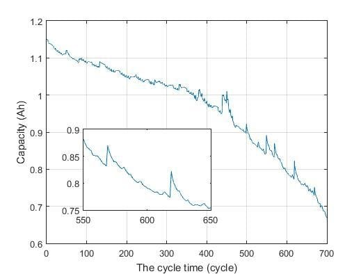
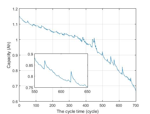
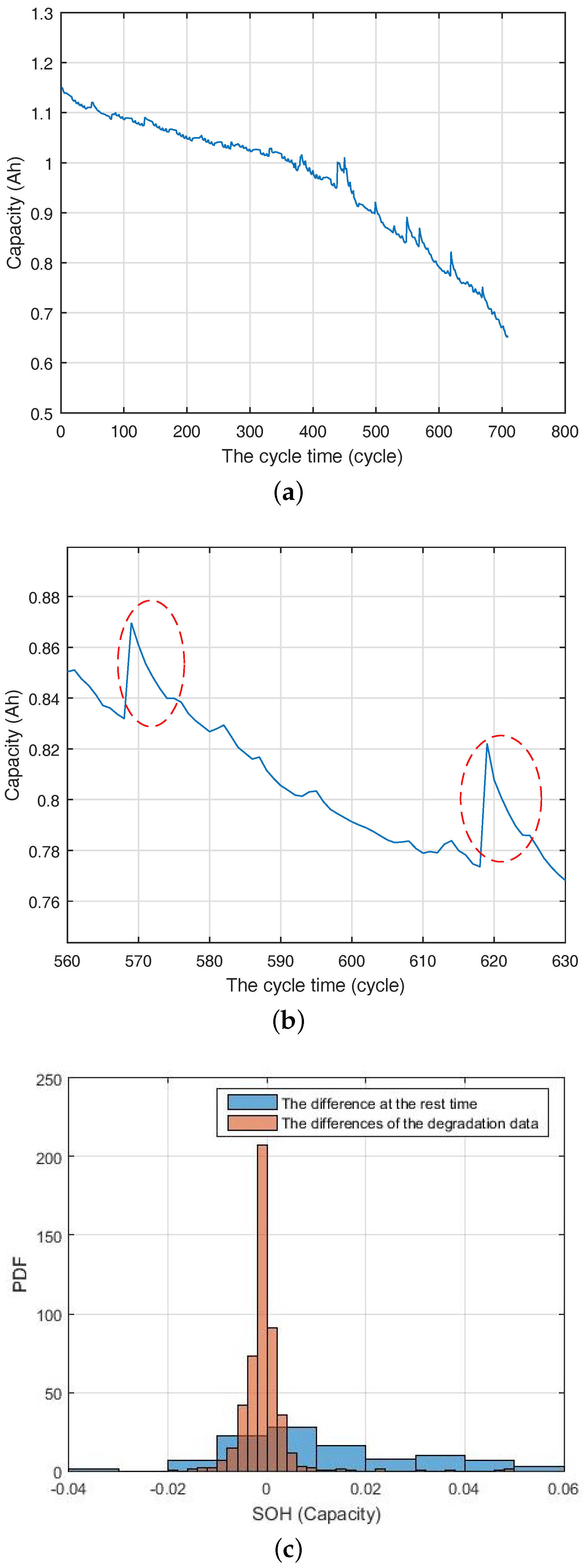
As discussed in the literature [3,11,26], the capacity of the battery will be likely to recover after the battery rests during the charge/discharge procedure. For example, the following Figure 1a shows a set of testing data of lithium-ion battery (i.e., CS2-34) collected by the Center for Advanced Life Cycle Engineering (CALCE) of Maryland University, where the battery is prismatic and its capacity is 1100 mAh. What should be noted is that its charging profile is a standard constant current/constant voltage protocol with a constant current rate of 0.5 C until the voltage reaches 4.2 V, and then 4.2 V is sustained until the charging current drops to below 0.05 A. From the degradation data, several aspects should be noticed,
- (1)
- In the testing data from CALCE, the rest time lasts several and even more hours, which is caused by the pause between two continuous charge/discharge tests. Therefore, we classify the degradation process of the battery into several phases according to the rest time.
- (2)
- The rest time does not only lead to regeneration phenomenon i.e., degradation state recovery but also unchanging and further deterioration. In Figure 1c, the blue lines denote the differences of the degradation data at the point of rest time, and the red lines represent the differences at other points, which are collected from the other four batteries CS2-35, CS2-36, CS2-37, CS2-38. It is interesting to note that the statistical histograms of these two differences data are distinguished obviously, including their means and variances. In another word, all regeneration phenomena occur at the rest time, but it does not mean that each testing rest leads to regeneration phenomenon.
- (3)
- When a regeneration phenomenon occurs, not only the degradation state will increase suddenly, but also the degradation rate changes as shown in Figure 1b, which is the enlarged figure of Figure 1a for better illustration. It is noteworthy that the degradation rate will first increase heavily after a regeneration phenomenon appears, and then decrease gradually and finally return to that at the end of the previous phase.
However, most researchers only focus on parts of these three aspects, and few of them take a full consideration of the above three aspects for degradation modeling and lifetime estimation. So, it is essential to build an appropriate degradation model to satisfy such three features, and then estimate the lifetime and RUL based on the proposed model. As such, we attempt to propose a multi-phase degradation model with random jumps to handle all characters of such the state-recovery degradation trajectory, which is formulated as follows.
2.2. Formulation and Degradation Modeling
In this paper, we focus on the degradation model based on the stochastic process and statistical analysis. Let denote the degradation process and then the lifetime, and then RUL under the concept of the FPT can be expressed as [9,27],
where denotes the failure threshold which is usually defined as a constant value and determined by engineering practical condition. Then we make represent the probability density function (PDF) of the lifetime and denote the cumulative distribution function (CDF). In addition, the RUL usually draws more attention for an operating system. As usual, the RUL under the concept of the FPT is often defined as,
where is the remaining useful life with PDF and CDF at time .
In order to attain the lifetime and RUL estimation under the concept of the FPT, it is essential to establish an appropriate degradation model to fit the degradation trajectory. It is noted that if the regeneration phenomena occur, both the degradation state and rate will be affected and changed. As discussed before, the regeneration phenomenon is mainly related to the testing rest. In this paper, we treat the influence of testing rest as the non-fatal random shock, which will change the degradation state and rate randomly. Hence, inspired by multi-phase degradation model as many literatures [25,28], we propose a novel multi-phase degradation model with random jumps as follows,
where denotes the degradation process, represents the traditional continuous degradation process without the effect of the testing rest, reflects the change of degradation state and rate caused by i-th testing rest. In this way, the degradation process can be classified into phases and each rest time can be regarded as the changing point, when there are times of testing rest. It is defined that the all changing point time is prearranged and denotes the current time of the i-th changing point. Then, Equation (3) can be written as follows,
where denotes total times of the changing points, i.e., .
It is noteworthy that the continuous degradation trajectory of battery is not monotone, which makes the degradation models based on the monotone stochastic process (such as Gamma process [29], Inverse Gaussian process [30] and so on) not suitable. In this case, due to the non-monotonicity of the degradation process, we adopt Wiener process to describe the continuous degradation process , and it holds the following form,
where is the initial value, t is the time, is the standard Brownian motion, and are purely time-dependent drift and diffusion coefficients.
Furthermore, based on the characters of the practical degradation data and inspired by the definition in [25,31], the negative exponential model is adopted to reflect the influence of the regeneration,
where denotes the time when the i-th testing rest occurs, represents the parameters. It is worth mentioning that reflects the sudden change of the degradation state caused by the testing rest, and describes its effect on the degradation rate. In order to better describe the randomness of the regeneration phenomena, it is assumed that and follow Gaussian distribution i.e., and .
Next, we will discuss how to derive the RUL estimation under the of the FPT for such the proposed multi-phase degradation model.
3. Remaining Useful Life Estimation under the Concept of the FPT
In this section, we concentrate on how to attain the RUL estimation under the concept of the FPT. It is noted that the derivation of the FPT is affected by the form of . In this case, for simplicity we assume that the occurrence time of the rest time is prearranged and it is defined as a fixed value. We define that there are times of rest time, i.e., . From Figure 2b, it could be found that the degradation rate will be increased suddenly and then recover gradually. As such, the following assumption is given,
Assumption A1.
It is assumed that each changed rate will recover to the initial value at the end of each degradation phase. That is to say, in Equation (6) will approach to 0 and have no impact on the -th phase, and only the effect of is accumulated.
It is noted that due to the random jump caused by the regeneration phenomena, so the estimated PDF of the lifetime or RUL are not continuous at the changing point. Under this consideration, we will calculate the form of the lifetime under the concept of the FPT separately in different intervals subject to the degradation phase, i.e., , and , where . Under the concept of the FPT, means that the FPT of the degradation process only belongs to , as well as and . For example, if , for the degradation . Therefore, we will attempt to derive the PDF of lifetime T in different intervals, i.e., , and , where .
First of all, we focus on the simplest case, i.e., . It is noteworthy that is only determined by the first degradation phase. Thus, we can easily obtain the expression of through the property of the Wiener process.
where denotes the initial value and it is often set as 0 for simplicity.
However, it is not easy to derive the at other intervals i.e., and directly. In order to derive at other intervals i.e., and , we first assume that denotes the degradation state at the changing point (or the rest time) . Furthermore, let be the left limit of , as well as .
Remark 1.
It is worth mentioning that represents the degradation state at time . In fact, the real cannot be known and should be a random variable which is determined by the degradation models of the first i phases. Due to the influence of the rest time, it is noted that the left limit is not equal to .
Then, under this assumption, degradation model at interval and can be written as follows,
where if the degradation belongs to , .
In this way, we can find that the degradation model at each phase except the first phase is nonlinear. To obtain the FPT of the nonlinear degradation model, following Lemma 1 based on the time-scale transformation is introduced,
Lemma 1.
[27]: If the degradation model is defined as , its approximate PDF of lifetime can be obtain as follows,
where . In this way, we can easily obtain the approximate PDF of lifetime with fixed and according to the conclusion of Lemma 1.
where or . As discussed before, , , and are random variables. To better illustrate, it is assumed that the PDFs of , , and are , , and . It is noted that represents the transition probability from to under the concept of the FPT. In this way, the approximate PDF of the lifetime can be obtained according to the law of total probability as shown in following equation.
where or , and follow Gaussian distribution, but is unknown. It is worth mentioning that the PDFs of the lifetime exhibits in a form of the triple integration corresponding to three random variables, i.e., , , and .
In order to obtain the PDF of lifetime, we must attain the PDF of . What should be noticed that can be also regarded as the transition probability under an absorbing boundary ξ. Unfortunately, the analytical form of is hard to calculate owing to the nonlinear degradation model and the random jumps. Here we introduce an approximate way to deal with it.
Define as the transition probability from to without the absorbing boundary. Then depending on the proposed degradation model and the property of the Wiener process, we can obtain the form of as shown in following equation,
where we let for simplicity, but . Then, we use to replace for deriving the lifetime estimation in Equation (11). In this case, by combing the results of Equations (7) and (11), we can obtain the approximate PDF of lifetime as follows,
where . In Equation (14), there are triple integrals needing to solve, which is similar to Equation (11) owing to three random variables. In order to simplify this integral, we introduce the following Theorem 1 based on the property of Gaussian distribution.
Theorem 1.
It is defined that and are two independent Gaussian random variables, and , , , , C, and D are fixed value. Then let , we can have the following results,
where
Proof.
See Appendix A.
In this way, we can solve the integral with and in Equation (14) depending on the results of Theorem 1 and then Equation (14) can be rewritten as follows,
where
However, it is not easy to obtain the analytical form of the above integrals. Fortunately, only univariate integral needs to be calculated, which can be solved by many numerical methods such as trapezoidal approximations, parabolas approximations, and Rhomberg integration.
It is noted that the time of the changing point is prearranged and known under the assumption, i.e., is prearranged. In practice, the rest time may not be provided or known in advance, and it is unknown and random. In this case, we define the PDF of each changing point as . Then, we can obtain the PDF of the lifetime based on the law of total probability.
where denotes the PDF of the lifetime with fixed changing point. In this way, the results under the prearranged changing point can be extended to the random case. For example, Zhang et al. [25] utilized the semi-Markov model (SMM) to reflect the degradation phase switch, and then generated the distribution of each changing time. Owing to the limitation of space, we do not further investigate how to formulate the framework of mode transitions (i.e., the rest time) in this paper. ☐
Now, we have completed the lifetime estimation based on the proposed multi-phase degradation model. In order to facilitate the application of our approach, we should discuss how to identify the model based on the collected data.
4. Parameter Estimation Based on the ECM Algorithm
In this section, we mainly focus on the model identification. Firstly, we attempt to formulate the likelihood function based on the property of the Wiener process.
We define that denotes the degradation data at time . For simplicity, we tranform into , where represents the j-th observation at i-th phase, and thus .
It is assumed that and are fixed, then the increment of observation data can be written as,
where .
However, due to the uncertainty of and , it is hard to formulate the likelihood function, and further the analytical solution of likelihood function cannot be obtained. As such, it is difficult to estimate the parameters via the traditional maximum likelihood estimation (MLE). In this case, it is natural to treat and as latent variables and adopt EM algorithm or its extended method for parameter estimation. It is well-known that two steps are included in the EM algorithm, i.e., E-step and M-step. Then we will introduce how to realize the model identification according to such two steps.
E-step: Let represent the latent variables. Then, if the latent variables are known, we can obtain the likelihood function as shown in Equation (21),
where denotes all parameters and is the observation of . Next, we calculate the conditional expectation of complete-data likelihood function,
where represents the all estimates in the m-th step based on .
It is noteworthy that and follow the Gaussian distribution and we only need to derive the expressions of , , , , and . In practice, the interval time is usually defined as a fixed value, thus we let for simplicity. Then, based on the Bayesian rule, following results for deriving can be obtained,
Proof.
See Appendix B.
In this way, the expression of has been attained. Then the next step is to maximize .
M-step: In order to maximize , the direct way is to make and then solve such the equation. In this way, we can obtain some solutions,
where the expressions of , , , , and can be found in Equation (23). It is noted that , , , and are global optimal solutions for maximizing .
However, only , , , and can be derived with an analytical forms, and other parameters i.e., μ, , and cannot be attained owing to the complexity of . If we choose some of the heuristic optimization methods to deal with it, not only is the existence and convergence of optimization for parameters estimating hard to analyze, but also the online capability will be poor. Under this consideration, we utilize the ECM algorithm to simplify the issue [32,33]. According to the ECM algorithm, we firstly fix and then derive the results of μ and , i.e., we treat as the real value of in this step. In this way, we can obtain analytical solutions of μ and as shown in follows,
where .
Then next step is to derive via maximizing , which can be formulated as,
In this way, compared with the traditional EM algorithm, ECM algorithm can reduce the number of parameters for optimization from 4 to in every M-step, which decreases the computing complexity and save the time. ☐
4.1. Implementation Procedure
In order to make the present results more feasible for engineering applications, a step-by-step procedures of the proposed approach with respect to model identification are developed in this subsection and summarized as shown in Table 1.
Following the above procedures, the proposed method can be established for model identification based on ECM algorithm.
5. Case Study
In this section, two examples are provided: (1) a numerical simulation is adopted to verify the accuracy of parameter estimation and the PDF of RUL; (2) The actual degradation data of battery is used to illustrate the feasibility of the proposed model.
5.1. Numerical Example
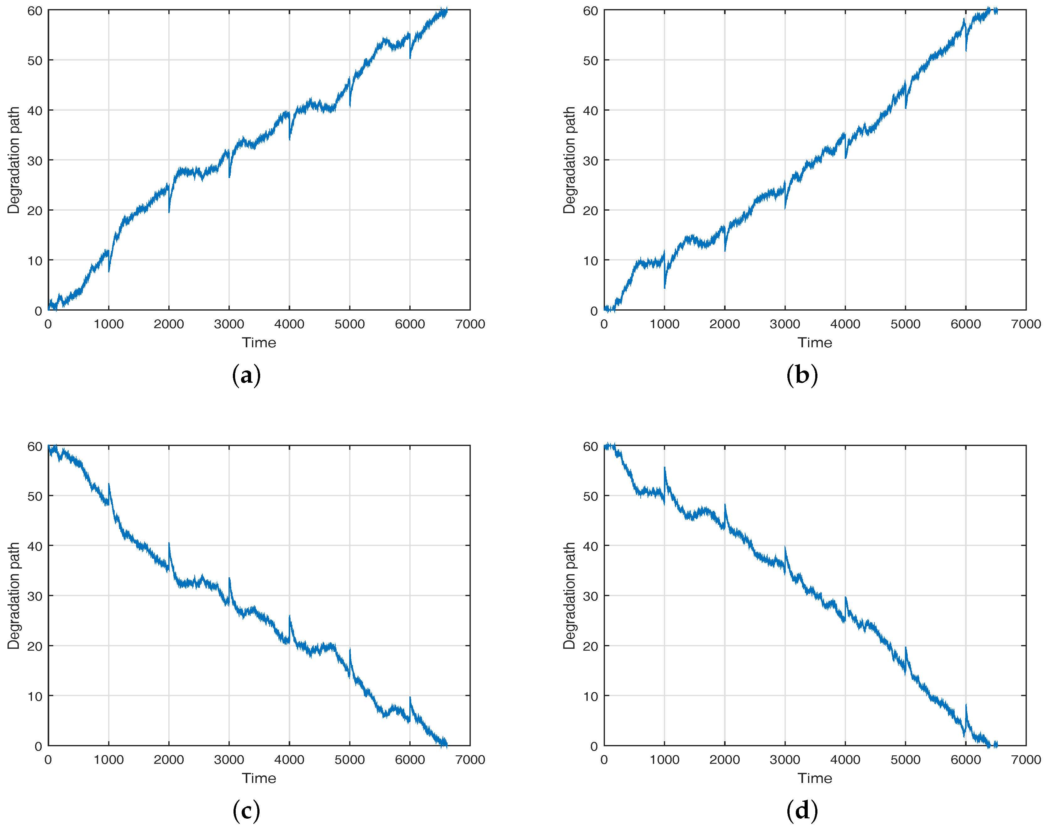
In this subsection, we concentrate on how to verify the reasonability and effectiveness of our theory, including the result of the approximate analytical lifetime estimation and the approach of parameter identification. Firstly, we will illustrate the method of lifetime estimation via comparing our results with those from Markov Chain Monte Carlo (MCMC). In this paper, two cases are taken into account: the fixed jump at the changing point and the random jump at the changing point. For the first case, we let , , , , and . For another case, we let , , , , , , and . According to the given parameters, we can further generate the degradation trajectories as shown in following Figure 2a,b. It is assumed that the failure threshold ξ is set at 60. It is interesting to be noted that if we make , the is similar to the practical degradation data as shown in Figure 1, where denotes degradation path we generated based on the proposed degradation model in Equation (3). In this way, the degradation can be transformed into the degradation process with initial value and threshold , and its degradation rate become negative. What should be noticed that such the transformation does affect the lifetime estimation under the concept of the FPT.
In addition, we adopt the MCMC to generate 1,000,000 sets of degradation trajectories based on our proposed model as shown in Equation (4) and collect their FPTs as the result of lifetime. Here these FPTs are regarded as the lifetime and then they will be compared with our theoretical results for illustration. In this way, we can obtain the results of our method and the MCMC separately, and the following Figure 3 shows the comparisons of the two aforementioned cases. The blue line denotes the results of the MCMC, and the red lines represent the results of our approach, and the green dotted lines are the results of the traditional way that ignores the influence of the regeneration. From the comparison as shown in Figure 3, we can notice that the results of our method are similar to those of the MCMC. It is interesting to be noteworthy that the deviations of lifetime estimation with fixed regeneration (or jump) are smaller than those with random regeneration owing to the uncertainty and randomness of and . In addition, we can find that the deviation of the traditional method is obvious, especially the estimated PDFs at the changing points. Thus, it could be concluded that our method can do lifetime estimation for the proposed degradation model under the concept of the FPT efficiently.
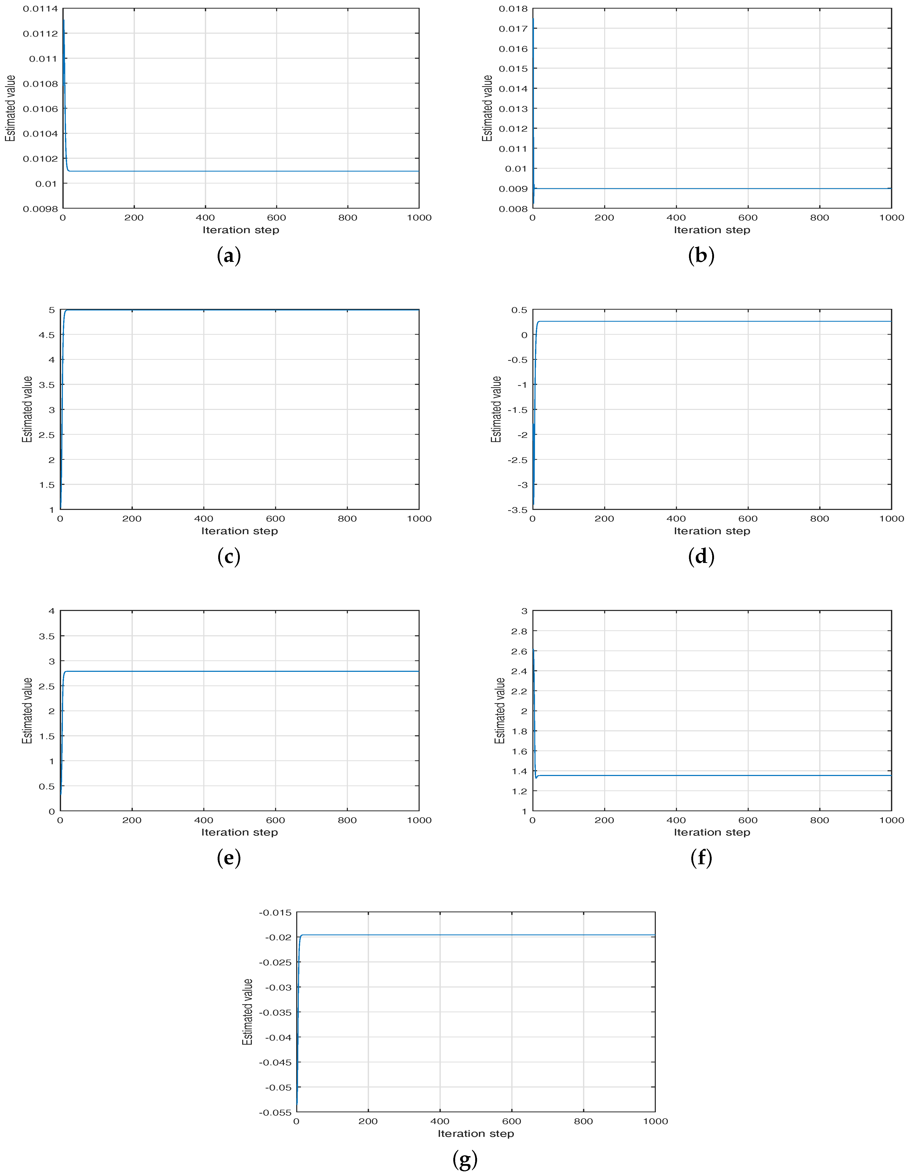
Next, we will introduce how to realize model identification based on our algorithm. According to the proposed method in Section 4, we generate 10 degradation trajectories with 10 times random regeneration phenomena, where the parameters are set as those in the above case 2 and the each degradation phase lasts 1000 time steps. In this case, all data can be converted to 100 phases. Based on the proposed approach, we can attain the parameters’ estimates as following table shown.
From Table 2, we find that our results approach the true value, which verifies the effectiveness of our method. It is worth mentioning that the initial value of all parameters are set as , , , , , , and . To better illustrate, we display each iteration of parameter estimation based on ECM algorithm as follows.
It could be found that the estimates of the all parameters can converge to the estimated value quickly with around 10 steps of iteration in Figure 4. It means that the online capability of the proposed method is good and acceptable.
Therefore, the numerical example can illustrate our approach in theory. Next we will apply our method into the practical case for showing its practical application.
5.2. Practical Example
In this case, we choose the testing data of Li-Ion battery collected by the Center for Advanced Life Cycle Engineering (CALCE) of Maryland University to verify our approach [3,34]. Here, we choose the CS2 battery to verify our method. It is noted that such the battery is prismatic and its cathode is LiCoO2. Its constant current rate is 0.5 C until the voltage reaches 4.2 V and then 4.2 V is sustained until the charging current drops to below 0.05 A. To better illustrate this, a set of degradation data is chosen to identify the model i.e., CS2-34, and its estimated parameters are provided for RUL estimation. According to the proposed method for model identification, the estimates of the all parameters are obtained as , , , , , , and . From the parameters’ estimates, it is noted that and it obviously larger than and the increment of the degradation data. That is to say, the regeneration phenomenon does exist in the degradation process, and the testing rest is a non-negligible factor of the regeneration phenomenon. Moreover, means that the degradation rate will suddenly increase and then gradually recover.
Next, based on the parameters’ estimates, we try to illustrate the RUL estimation based on the proposed method. It is well-known that a certain percentage of the rated capacity is treated as the soft failure threshold of the battery. In this paper, we set the failure threshold at of the rated capacity to better illustrate the effect caused by the regeneration phenomena, i.e., the failure threshold . Furthermore, what should be noticed is that the rest time of this degradation process is known. In another word, the changing time has been prearranged. In this way, combining the prior value of parameters and the failure threshold, we can obtain the PDFs of RUL for CS2-34 as shown in following Figure 5. What should be noticed is that the estimated RUL is a random distribution rather than a fixed value. So we choose the mean square error (MSE) to reflect the error as shown in Figure 5b.
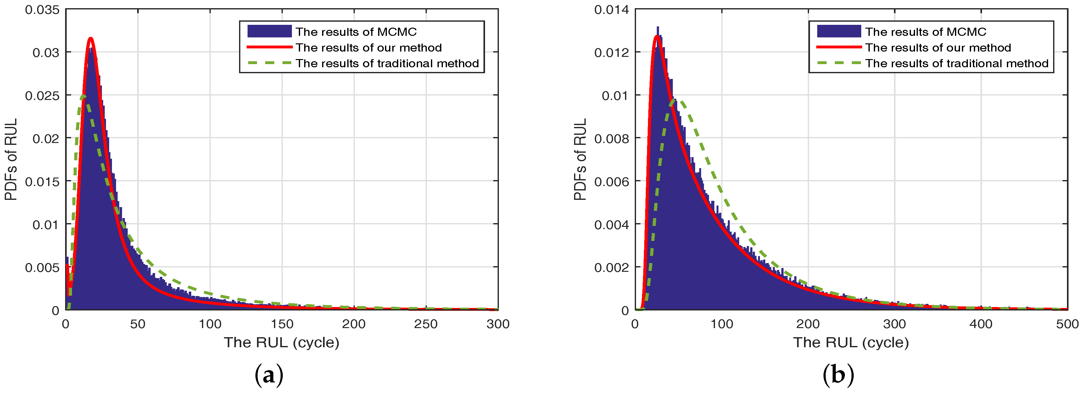
From Figure 5, we can find that compared to the traditional method the results of our method can approach the true RUL with smaller estimated bias, since we take full consideration of the influence of such the regeneration phenomena. It is noted that if the regeneration phenomena are ignored, the estimated RUL will be influenced by the random jumps heavily, and the result will be overestimated owing to the state recovery, i.e., the estimated RUL become longer. In contrast, because our method has fully considered the effects of the regeneration phenomena on both degradation state and rate, the results of our method could be less affected. In order to better illustrate, we compare the PDFs of our method and the traditional method at the beginning and end of a degradation phase accordingly. The following Figure 6 shows that the PDFs of estimated RUL at cycle time 568 and 569.
It is noticed that the estimated bias between our result and traditional method at the cycle time 568 is smaller than cycle time 569. That is to say, the result of the traditional method may have much more bias at the beginning of the degradation phase since it is susceptible to the regeneration phenomena. Therefore, it can be concluded that the regeneration will influence the lifetime and RUL estimation, and the traditional method cannot deal with it well. On contrary, our method can not only reflect the degradation trajectory but also achieve more accurate estimated result, which illustrates the advantage and effectiveness of our approach.
6. Conclusions
In this paper, we mainly concentrate on how to model the degradation process with state-recovery phenomena. Under this consideration, we propose a multi-phase degradation with random jumps to describe such the degradation trajectory. In the proposed model, we classify the degradation process into several phases according to the rest time, and take a full account of the uncertainty of regeneration phenomena. Then we develop a model identification method based on the ECM algorithm to deal with complex likelihood function and the random latent variables. Furthermore, according to the proposed degradation model, we derive the lifetime estimation based on the time-scale transformation and law of total probability, and then obtain an approximate solution with the form of an single integral. To better illustrate our method, both numerical example and the practical example of CALCE batteries are adopted for demonstration.
Although the proposed method can better describe the degradation with regeneration phenomena and provide accurate lifetime estimation, there are still some problems needing to be investigated in the future. First, in this paper, we assume the rest time is prearranged, but the appearance of the rest time may be random and uncertain in practice. As such, in future work, we will try to formulate a framework of random operating state switches (i.e., the rest time), and then extended our approach for lifetime or RUL estimation to the stochastic case. Second, the changing degradation rate caused by the regeneration phenomena is a fixed value in our model. In fact, the changing degradation rate (i.e., the degradation rate at every phase) should exist difference between different degradation phases. Maybe, the random rate which can describe the phase-to-phase variability is more suitable. Third, it is noteworthy that the environmental temperature of the testing data we adopted does not change heavily so that we ignore its influence in this paper. However, the ambient temperature often change constantly in practice, which will affect the batteries’ degradation rate and fluctuation. We will continue to investigate such these issues in future work.
Acknowledgments
This work was supported by National Natural Science Foundation of China (NSFC) under Grants 61490701, 61573365, 61773386, and Tsinghua University Initiative Scientific Research Program. The work of Xiao He was also supported by the NSFC under Grant 61473163, 61522309 and 61733009. The work of Xiaosheng Si was also supported by the NSFC under Grant 61374126, 61473094, 61573076, 61673311, and Young Elite Scientists Sponsorship Program (YESS) of China Association for Science and Technology (CAST) under grant 2016QNRC001.
Author Contributions
Jianxun Zhang completed the theoretical analysis, and wrote the paper; Changhua Hu and Donghua Zhou formulated the framework, and structured the whole manuscript. Xiao He and Xiaosheng Si checked the results, and revised the paper.
Conflicts of Interest
The authors declare no conflict of interest.
Abbreviations
The following abbreviations are used in this manuscript:
| RUL | Remaining useful life |
| MLE | Maximum Likelihood Estimation |
| EM | Expectation maximum |
| ECM | Expectation conditional maximum |
| SOH | State of health |
| PHM | Prognostic and health management |
| FPT | First passage time |
| CALCE | Center for Advanced Life Cycle Engineering |
| Probability density function | |
| CDF | Cumulative distribution function |
| SMM | Semi-Markov model |
| MCMC | Markov Chain Monte Carlo |
Notation
| T | The lifetime |
| The RUL at time | |
| The whole degradation process | |
| The continuous degradation process without the effect of the regeneration phenomenon | |
| The changing degradation process caused by the i-th testing rest | |
| The occurrence number of testing rest at time t | |
| The occurrence time of i-th testing rest | |
| Total times of the testing rest | |
| The drift coefficient | |
| The diffusion coefficient | |
| The standard Brownian motion | |
| The initial value of degradation process | |
| The parameters of the model of the regeneration phenomenon | |
| , | The mean and variance of |
| , | The mean and variance of |
| The failure threshold | |
| The PDF of the lifetime | |
| The degradation state at time t | |
| The left limit of | |
| The j-th observation at i-th phase | |
| The difference of | |
| The difference of t | |
| , | Two functions of the time t |
| The transition probability from to under the concept of the FPT | |
| , | The PDFs of and |
| Take the expectation of | |
| The all parameters of the proposed model | |
| The estimate of | |
| The estimate of at the m-th iteration | |
| The all degradation observation data |
Appendix A
It is defined that and are two independent Gaussian random variables with PDFs and accordingly, and , , , , C, and D are fixed value.
Firstly, we will calculate the
where we can utilize the method of completing the square to obtain the solutions of , , and E.
It is noted that is not relevant to and , and can be regarded as a PDF of bivariate normal distribution. Then according to the bivariate normal distribution, we can further obtain,
Then based on the property of the bivariate normal distribution, the following solutions can be derived,
In this way, the proof has been completed.
Appendix B
It is noted that and in Equation (22) can be regarded as the observations of and . According to and , we can further derive based on the property of the bivariate normal distribution. The detailed derivation procedure is displayed as follows,
In this way, we can further obtain,
In the above equation, we should calculate , , , , and . Under such the consideration, we firstly derive the expression of . It is worth mentioning that and are only relevant to . Therefore, we can have . According to the Bayesian rule, we can obtain,
What should be noticed is that due to and , the can be transformed as the PDF of bivariate normal distribution. In this case, based on the method of completing square, we can derive the expression of as follows,
where
Further, based on the property of bivariate normal distribution, , , , , and . Under such the consideration, we firstly derive the expression of . It is worth mentioning that and are only relevant to . Therefore, we can have can be derived as follows,
In this way, the proof has been completed.
References
- Zhang, J.; Lee, J. A review on prognostics and health monitoring of Li-ion battery. J. Power Sources 2011, 196, 6007–6014. [Google Scholar] [CrossRef]
- Abada, S.; Marlair, G.; Lecocq, A.; Petit, M.; Sauvant-Moynot, V.; Huet, F. Safety focused modeling of lithium-ion batteries: A review. J. Power Sources 2016, 306, 178–192. [Google Scholar] [CrossRef]
- He, W.; Williard, N.; Osterman, M.; Pecht, M. Prognostics of lithium-ion batteries using extended Kalman filtering. In Proceedings of the IMAPS Advanced Technology Workshop on High Reliability Microelectronics for Military Applications, Linthicum Heights, MD, USA, 17–19 May 2011; pp. 17–19. [Google Scholar]
- Si, X.S. An adaptive prognostic approach via nonlinear degradation modeling: Application to battery data. IEEE Trans. Ind. Electron. 2015, 62, 5082–5096. [Google Scholar] [CrossRef]
- Pecht, M. Prognostics and Health Management of Electronics; Wiley Online Library: Hoboken, NJ, USA, 2008. [Google Scholar]
- Zhang, J.X.; Hu, C.H.; He, X.; Si, X.S.; Liu, Y.; Zhou, D.H. Lifetime prognostics for deteriorating systems with time-varying random jumps. Reliab. Eng. Syst. Saf. 2017, 167, 338–350. [Google Scholar] [CrossRef]
- Tsui, K.L.; Chen, N.; Zhou, Q.; Hai, Y.; Wang, W. Prognostics and health management: A review on data driven approaches. Math. Probl. Eng. 2015, 2015, 1–17. [Google Scholar] [CrossRef]
- Zio, E. Prognostics and health management of industrial equipment. In Diagnostics and Prognostics of Engineering Systems: Methods and Techniques; IGI Global: Hershey, PA, USA, 2012; pp. 333–356. [Google Scholar]
- Si, X.S.; Wang, W.; Hu, C.H.; Zhou, D.H. Remaining useful life estimation—A review on the statistical data driven approaches. Eur. J. Oper. Res. 2011, 213, 1–14. [Google Scholar] [CrossRef]
- Jardine, A.K.; Lin, D.; Banjevic, D. A review on machinery diagnostics and prognostics implementing condition-based maintenance. Mech. Syst. Signal Process. 2006, 20, 1483–1510. [Google Scholar] [CrossRef]
- Liu, D.; Pang, J.; Zhou, J.; Peng, Y.; Pecht, M. Prognostics for state of health estimation of lithium-ion batteries based on combination Gaussian process functional regression. Microelectron. Reliab. 2013, 53, 832–839. [Google Scholar] [CrossRef]
- Tang, S.; Yu, C.; Wang, X.; Guo, X.; Si, X. Remaining useful life prediction of lithium-ion batteries based on the wiener process with measurement error. Energies 2014, 7, 520–547. [Google Scholar] [CrossRef]
- Hu, C.; Youn, B.D.; Chung, J. A multiscale framework with extended Kalman filter for lithium-ion battery SOC and capacity estimation. Appl. Energy 2012, 92, 694–704. [Google Scholar] [CrossRef]
- Dalal, M.; Ma, J.; He, D. Lithium-ion battery life prognostic health management system using particle filtering framework. Proc. Inst. Mech. Eng. Part O J. Risk Reliab. 2011, 225, 81–90. [Google Scholar] [CrossRef]
- Saha, B.; Goebel, K.; Poll, S.; Christophersen, J. Prognostics methods for battery health monitoring using a Bayesian framework. IEEE Trans. Instrum. Meas. 2009, 58, 291–296. [Google Scholar] [CrossRef]
- Song, Y.; Liu, D.; Yang, C.; Peng, Y.; Horaud, R.; Forbes, F.; Yguel, M.; Dewaele, G.; Zhang, J. Data-driven hybrid remaining useful life estimation approach for spacecraft lithium-ion battery. Microelectron. Reliab. 2017, 75, 142–153. [Google Scholar]
- Panchal, S.; Dincer, I.; Agelin-Chaab, M.; Fraser, R.; Fowler, M. Experimental and simulated temperature variations in a LiFePO 4-20Ah battery during discharge process. Appl. Energy 2016, 180, 504–515. [Google Scholar] [CrossRef]
- Panchal, S.; Mcgrory, J.; Kong, J.; Fraser, R.; Fowler, M.; Dincer, I.; Agelin-Chaab, M. Cycling degradation testing and analysis of a LiFePO4 battery at actual conditions. Int. J. Energy Res. 2017, 1. [Google Scholar] [CrossRef]
- Williard, N.; He, W.; Hendricks, C.; Pecht, M. Lessons learned from the 787 dreamliner issue on lithium-ion battery reliability. Energies 2013, 6, 4682–4695. [Google Scholar] [CrossRef]
- Guo, J.; Li, Z.; Pecht, M. A Bayesian approach for Li-Ion battery capacity fade modeling and cycles to failure prognostics. J. Power Sources 2015, 281, 173–184. [Google Scholar] [CrossRef]
- Olivares, B.E.; Munoz, M.A.C.; Orchard, M.E.; Silva, J.F. Particle-filtering-based prognosis framework for energy storage devices with a statistical characterization of state-of-health regeneration phenomena. IEEE Trans. Instrum. Meas. 2013, 62, 364–376. [Google Scholar] [CrossRef]
- He, Y.J.; Shen, J.N.; Shen, J.F.; Ma, Z.F. State of health estimation of lithium-ion batteries: A multiscale Gaussian process regression modeling approach. AIChE J. 2015, 61, 1589–1600. [Google Scholar] [CrossRef]
- Orchard, M.E.; Lacalle, M.S.; Olivares, B.E.; Silva, J.F.; Palma-Behnke, R.; Estévez, P.A.; Severino, B.; Calderon-Muñoz, W.; Cortés-Carmona, M. Information-theoretic measures and sequential monte carlo methods for detection of regeneration phenomena in the degradation of lithium-ion battery cells. IEEE Trans. Reliab. 2015, 64, 701–709. [Google Scholar] [CrossRef]
- Qin, T.; Zeng, S.; Guo, J.; Skaf, Z. A Rest Time-Based Prognostic Framework for State of Health Estimation of Lithium-Ion Batteries with Regeneration Phenomena. Energies 2016, 9, 896. [Google Scholar] [CrossRef]
- Zhang, Z.X.; Si, X.S.; Hu, C.H.; Pecht, M.G. A Prognostic Model for Stochastic Degrading Systems with State Recovery: Application to Li-Ion Batteries. IEEE Trans. Reliab. 2017, 1–6. [Google Scholar] [CrossRef]
- Saha, B.; Goebel, K. Modeling Li-ion battery capacity depletion in a particle filtering framework. In Proceedings of the Annual Conference of the Prognostics and Health Management Society, San Diego, CA, USA, 27 September–1 October 2009; pp. 2909–2924. [Google Scholar]
- Si, X.S.; Wang, W.; Hu, C.H.; Zhou, D.H.; Pecht, M.G. Remaining useful life estimation based on a nonlinear diffusion degradation process. IEEE Trans. Reliab. 2012, 61, 50–67. [Google Scholar] [CrossRef]
- Kong, D.; Balakrishnan, N.; Cui, L. Two-Phase Degradation Process Model with Abrupt Jump at Change Point Governed by Wiener Process. IEEE Trans. Reliab. 2017. [Google Scholar] [CrossRef]
- Chen, N.; Ye, Z.S.; Xiang, Y.; Zhang, L. Condition-based maintenance using the inverse Gaussian degradation model. Eur. J. Oper. Res. 2015, 243, 190–199. [Google Scholar] [CrossRef]
- Lawless, J.; Crowder, M. Covariates and random effects in a gamma process model with application to degradation and failure. Lifetime Data Anal. 2004, 10, 213–227. [Google Scholar] [CrossRef] [PubMed]
- Chaari, R.; Briat, O.; Vinassa, J.M. Capacitance recovery analysis and modelling of supercapacitors during cycling ageing tests. Energy Convers. Manag. 2014, 82, 37–45. [Google Scholar] [CrossRef]
- Nagaraju, V.; Fiondella, L.; Zeephongsekul, P.; Jayasinghe, C.L.; Wandji, T. Performance Optimized Expectation Conditional Maximization Algorithms for Nonhomogeneous Poisson Process Software Reliability Models. IEEE Trans. Reliab. 2017, 66, 722–734. [Google Scholar] [CrossRef]
- Horaud, R.; Forbes, F.; Yguel, M.; Dewaele, G.; Zhang, J. Rigid and articulated point registration with expectation conditional maximization. IEEE Trans. Pattern Anal. Mach. Intell. 2011, 33, 587–602. [Google Scholar] [CrossRef] [PubMed] [Green Version]
- Pecht, M. CALCE Battery Group. Available online: http://www.calce.umd.edu/batteries/data.htm (accessed on 11 September 2017).
Figure 1.
The degradation trajectory of the battery. (a) The degradation of battery capacity; (b) The regeneration phenomena in the degradation process; (c) The degradation difference between the rest time and others.
Figure 1.
The degradation trajectory of the battery. (a) The degradation of battery capacity; (b) The regeneration phenomena in the degradation process; (c) The degradation difference between the rest time and others.

Figure 2.
The simulated degradation trajectories generated from the proposed model. (a) The degradation trajectory with fixed regeneration; (b) The degradation trajectory with random regeneration; (c) The degradation trajectory with negative rate and fixed regeneration; (d) The degradation trajectory with negative rate and random regeneration.

Figure 3.
The comparison of lifetime estimation. (a) The comparison of PDFs with fixed jumps; (b) The comparison of PDFs with random jumps.
Figure 3.
The comparison of lifetime estimation. (a) The comparison of PDFs with fixed jumps; (b) The comparison of PDFs with random jumps.
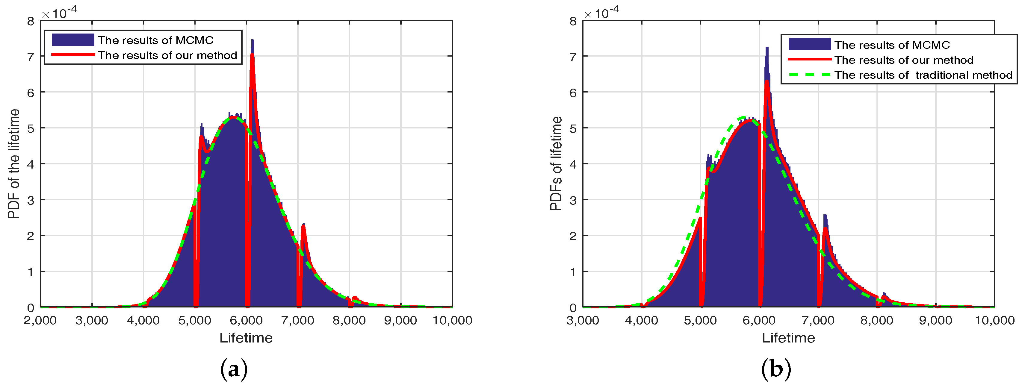
Figure 4.
The iterations of estimated parameters based on ECM algorithm. (a) The iteration of ; (b) The iteration of ; (c) The iteration of ; (d) The iteration of ; (e) The iteration of ; (f) The iteration of ; (g) The iteration of .
Figure 4.
The iterations of estimated parameters based on ECM algorithm. (a) The iteration of ; (b) The iteration of ; (c) The iteration of ; (d) The iteration of ; (e) The iteration of ; (f) The iteration of ; (g) The iteration of .

Figure 5.
The comparison of the estimated RUL. (a) The comparison of expectation of RUL; (b) The MSE of estiamted RUL.
Figure 5.
The comparison of the estimated RUL. (a) The comparison of expectation of RUL; (b) The MSE of estiamted RUL.
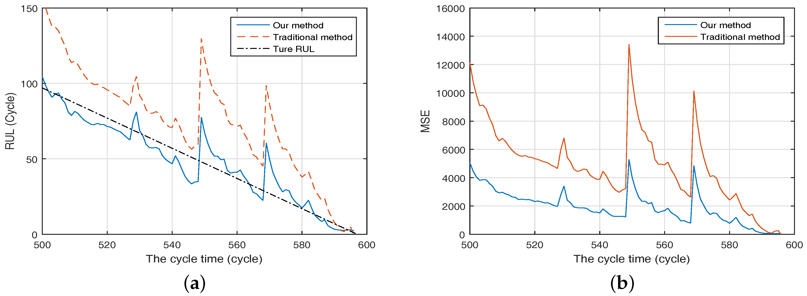
Figure 6.
The comparison of PDFs of the estimated RUL at two different cycle. (a) The PDFs of RUL at cycle 568; (b) The PDFs of RUL at cycle 569.
Figure 6.
The comparison of PDFs of the estimated RUL at two different cycle. (a) The PDFs of RUL at cycle 568; (b) The PDFs of RUL at cycle 569.

Table 1.
The implementation procedures of model identification.
| Algorithm Procedure: | |
|---|---|
| Step 1. | Collect the degradation data , and then obtain the occurrence number of rest time, i.e., ; |
| Step 2. | Transform into according to , and then obtain the difference of total observed data , where represents the j-th observation at i-th phase; |
| Step 3. | Regard and as the latent variables, and formulate the complete-data likelihood as shown in Equation (21). Let , and give the initial value .; |
| Step 4. | Calculate the conditional expectation of Equation (21), and then attain as shown in Equation (22), where denotes the estimates of all parameters at m-th iteration; |
| Step 5. | Fix , and obtain the estimates of other parameters via maximizing , where denotes all parameters except . Then the results can be found in Equations (24)–(26); |
| Step 6. | Fix , and derive via maximizing , which can be found in Equation (27); |
| Step 7. | Let , and repeat Step 4 to Step 6 until the estimates becomes convergence. Then such can be treated as the final estimates of . |
Table 2.
The parameters estimation with different sample size.
| Sample Size | ||||||||
|---|---|---|---|---|---|---|---|---|
| 2 | 0.0205 | 0.149 | 4.541 | −0.289 | 2.898 | 1.491 | 0.0204 | |
| 3 | 0.0148 | 0.072 | 4.516 | −0.214 | 2.720 | 1.428 | 0.0210 | |
| 4 | 0.0101 | 0.095 | 4.987 | 0.261 | 2.789 | 1.342 | 0.0196 | |
| 5 | True value | 0.0100 | 0.100 | 5.000 | 0.000 | 3.000 | 1.000 | 0.0200 |
© 2017 by the authors. Licensee MDPI, Basel, Switzerland. This article is an open access article distributed under the terms and conditions of the Creative Commons Attribution (CC BY) license (http://creativecommons.org/licenses/by/4.0/).
Share and Cite
MDPI and ACS Style
Zhang, J.; He, X.; Si, X.; Hu, C.; Zhou, D. A Novel Multi-Phase Stochastic Model for Lithium-Ion Batteries’ Degradation with Regeneration Phenomena. Energies 2017, 10, 1687. https://doi.org/10.3390/en10111687
AMA Style
Zhang J, He X, Si X, Hu C, Zhou D. A Novel Multi-Phase Stochastic Model for Lithium-Ion Batteries’ Degradation with Regeneration Phenomena. Energies. 2017; 10(11):1687. https://doi.org/10.3390/en10111687
Chicago/Turabian StyleZhang, Jianxun, Xiao He, Xiaosheng Si, Changhua Hu, and Donghua Zhou. 2017. "A Novel Multi-Phase Stochastic Model for Lithium-Ion Batteries’ Degradation with Regeneration Phenomena" Energies 10, no. 11: 1687. https://doi.org/10.3390/en10111687
Note that from the first issue of 2016, this journal uses article numbers instead of page numbers. See further details here.