Control Applied to a Reciprocating Internal Combustion Engine Test Bench under Transient Operation: Impact on Engine Performance and Pollutant Emissions

Abstract

This work presents a methodology to adjust the electronic control system of a reciprocating internal combustion engine test bench and the effect of the control parameters on emissions produced by the engine under two extreme situations: unadjusted and adjusted, both under transient operation. The aim is to provide a tuning guide to those in charge of this equipment not needed to be experts in control engineering. The proposed methodology covers from experimental plant modelling to control parameters determination and experimental validation. The methodology proposed includes the following steps: (i) Understanding of test bench and mathematical modeling; (ii) Model parameters identification; (iii) Control law proposal and tuning from simulation and (iv) Experimental validation. The work has been completed by presenting a comparative experimental study about the effect of the test bench control parameters on engine performance profiles (engine speed, engine torque and relative fuel air ratio) and on regulated gaseous emissions (nitrogen oxides and hydrocarbons concentrations) and the profile of number of particles emitted. The whole process, including experimental validation, has been carried out in a test bench composed of a turbocharged, with common rail injection system, light duty diesel engine coupled to a Schenck E-90 eddy current dynamometric brake and its related Schenk X-act control electronics. The work demonstrates the great effect of the test bench control tuning under transient operation on performance and emissions produced by the engine independently of the engine accelerator position demanded before and after the test bench tuning.

1. Introduction

Nowadays, the applications of electronic control to the operating processes of engines and vehicles are varied. Fathi et al. [1] have recently published an important review about works related to modelling and design of controller structure for controlling the known homogenous charge compression ignition. This work outlines, among others, from works dedicated to the denominated black-box modelling based on artificial networks [2] or based on system identification models [3] to those works about current controllers based on both linear [4,5] and non-linear models [6,7].

Other works have focused the application of electronic control techniques directly on Diesel engines with the objective of reducing fuel consumption and pollutant emissions by means of a switching strategy between both the high and low pressure exhaust gas recirculation systems [8] or acting on the exhaust gas recirculation (EGR) control strategy [9] or simply improving the intake air control system of engines [10,11].

In other cases, different EGR and injection strategies have been compared in order to study the effect of biodiesel fuels on performance and emissions of Diesel light-duty engines [12].

No less important have been those works related to the assessment of other types of techniques, as the use of biharmonic maps, to predict performance and emissions of vehicles working in captive fleets. In this work authors indicated the possibility of introducing the use of this technique in ECU operation [13].

Currently, although the literature dedicated to electronic control applied to the internal combustion engines is extensive, literature focused on the control system of the test bench itself (the engine + dynamometer brake set) is really insufficient. Included in this group of works, for example, Gotfryd [14] worked on the adaptation of an existing direct current (DC) dynamometer to transient operation in order to facilitate at least preliminary transient tests carried on for low-budget engine development purposes, while other authors worked directly on the improvement of the test bench control system [15,16,17].

Recent works have been published on the control of engine test benches, related to different studies cases: in [18] the authors proposed a nonlinear output feedback controller based on a reduced order observer to solve a set point tracking problem of a combustion engine test bench; in [19] an active vibration damping method through specific control of the dynamometric brake based on a Kalman filter was proposed; and in [20] a test bench control was simulated, including, in addition to the combustion engine test bench, the transmission model and the dynamic of the vehicle.

The present work can be included in the last mentioned group of works. In this case a combined theoretical-experimental methodology for the optimization of the control system of a reciprocating engine test bench is presented. The work done demonstrates the impact of the regulation of the engine test bench control system on performance and pollutant emissions produced by a light duty common rail diesel engine during different sequences under transient operation. Methodology proposed is integrated by different parts which includes from the plant (engine-dynamometer) modelling until the effect of the control system before and after the optimization on performance and main regulated pollutant emissions. Results show the great effect of the engine test bench control system on emissions if it is regulated without optimization. Finally, as collateral result, the methodology has additional advantage: its easy implementation by researchers without wide experience in optimization of automatic control systems.

2. Experimental Installation

Figure 1 shows a complete scheme of the experimental installation used in this work. The work was carried out in a test bench mainly composed by an engine coupled to a dynamometric brake. The engine was a four-stroke, 2.2 L, light-duty Diesel engine (NISSAN, Nissan Technical Centre Europe (NTCE), Barcelona, Spain) with four cylinders, turbocharged, intercooled and with a common-rail injection system. This engine (see main specifications in

Table 1. Main engine characteristics.

Type	Diesel, Direct Injection
Model	Nissan YD22
Total displacement	2.2 L
Cylinder arrangement	4 cylinders, in line
Bore/stroke	86.5/94 mm
Compression ratio	16.7:1
Intake system	Turbocharged with intercooler
EGR system	Hot, high pressure
Fuel injection system	Common rail, pilot injection
Maximum rated power	82 kW at 4000 min−1
Maximum rated torque	248 Nm at 2000 min−1

) is representative of those typical used in Diesel vehicles in Europe.

The engine was instrumented to measure several key temperatures and pressures (intake air, fuel, exhaust gases, lube oil, etc.). A piezoelectric pressure transducer (6056A, Kistler, Winterthur, Switzerland) coupled to a charge amplifier (Kistler 5018A, Winterthur, Switzerland) was used for recording instantaneous in-cylinder pressure. Crankshaft rotational speed and instantaneous piston position were determined with two possibilities: (i) by means of an angle encoder (Kistler 2614CK, Winterthur, Switzerland) with a resolution of 720 pulses per revolution and (ii) by means of the INCA PC (measurement, calibration and diagnostic software published by ETAS, Stuttgart, Germany) directly registered from the engine Electronic Control Unit (ECU). The data were recorded with a digital scope (DL708E, Yokowaga, Singapore) and transferred to the computer via general purpose interface bus (GPIB).

The engine was coupled to a Schenck E-90 eddy current dynamometer (Horiba Schenck, Landwehrstrasse 55, D-64293, Darmstadt, Germany). The brake control system allowed to measure and/or control the engine speed (ω), accelerator position (α) and engine torque (M). Maximum speed of the dynamometer is 12,000 min⁻¹ while the maximum torque is 200 Nm at 90 kW [21,22]. The test bench has an X-Act brake control system [23,24]. A widely used controller that implements the control scheme described in this work (see Appendix B). This controller is connected with a accelerator position controller.

A digital encoder coupled to the engine crankshaft shaft allowed to measure engine speed with resolution 720 pulses per turn. Electronic transducer gives measured engine speed signal (ω).

A load cell mounted on the engine-brake coupling shaft allowed to register the steady state engine torque signal (M) with resolution 0.4 Nm. Measurement error due to temperature is less than 2 Nm if temperature varies less than 10 °C from calibration.

In addition, in order to see the effect of control parameters of the test bench on pollutant emissions produced by the engine under a typical transient sequence, both, instantaneous concentration of gaseous pollutant emissions (nitrogen oxides, NO_x and unburned total hydrocarbons, THC) and instantaneous particle concentration were registered. Unburned total hydrocarbon emissions were measured with a flame ionization detector (model GRAPHITE 52M (Environnement, 111, Bd Robespierre—BP 84513, Poissy, France)) and a chemiluminiscence analyzer (model TOPAZE 32M (Environnement, 111, Bd Robespierre—BP 84513, Poissy, France)) was used to measure NO_x emissions. Instantaneous particle concentration was measured by means of a PEGASOR Particle Sensor (VP Sales & Marketing Pegasor Ltd., Tampere, Finland) model PPS-M.

As test fuel was used an ultra-low sulfur EN-590 Diesel fuel. Main properties of the test fuel are shown in

Table 2. Properties of the test fuel.

Properties	Diesel
Molecular formula	C15.18H29.13
Molecular weight (g/mol)	211.4
H/C Ratio	1.92
Stoichiometric fuel/air ratio	1/14.64
C (% w/w)	86.13
H (% w/w)	13.87
O (% w/w)	0
Density at 15 °C (kg/m3)	843
Viscosity at 40 °C (cSt)	2.97
Lower Heating Value (MJ/kg)	42.43
Cetane number	54.2
Cold filter plugging point (CFPP) (°C)	−17
Distillation (vol.)
10%	207.6
50%	278.2
90%	345.0

.

3. Methodology

The main goals of the test bench control system are to adjust brake opposition torque and speed, both under both steady and transient operating modes. Under transient operation, control avoids overshooting and warranties settle time of controlled signals. Under steady-state operating mode, control minimizes error between required and measured controlled signals.

These goals are obtained by two uncoupled control laws [16] of engine torque and engine speed. Control laws are obtained through a process of modeling and simulation of the whole test bench.

A reciprocating internal combustion engine is a complex thermodynamic system. Its performance depends on many different factors as density and temperature of the intake air, pressures and temperatures of several components of the engine, quality of the fuel, etc. Nevertheless, in a simple way the engine can be modeled as a linear first order system, although non linearity introduced by some elements such as the turbocharger and the electronic control unit (ECU) [17] have to be considered when analyzing simulation results.

Main signals to define the test bench operating mode are the following: (i) accelerator position $\left(\mathsf{\alpha }\right)$, measured in %; (ii) Engine speed $\left(\mathsf{\omega }\right)$, measured in min⁻¹ and (iii) Load cell torque, measured in Nm. The test bench control mode selected in this work has been $\raisebox{1ex}{$\mathsf{\alpha }$}\!\left/ \!\raisebox{-1ex}{$\mathsf{\omega }$}\right.$ mode. In this mode, the input parameter is $\mathsf{\alpha }$ and the demand is $\mathsf{\omega }$. Control acts on the brake to adjust the effective torque ${\mathrm{M}}_{\mathrm{F}}$ (opposition torque generated by the brake) to obtain the required $\mathsf{\omega }$.

In this section, a procedure for tuning the test bench control system is proposed. The main steps of this procedure can be summarized as follows: (i) Identification of the mechanical plant structure (test bench components and working modes); (ii) Modelling the mechanical plant and identification of its parameters and (iii) Obtaining the values of the plant control parameters. In this work we consider that control laws are implemented in the control system and we are allowed just to adjust them.

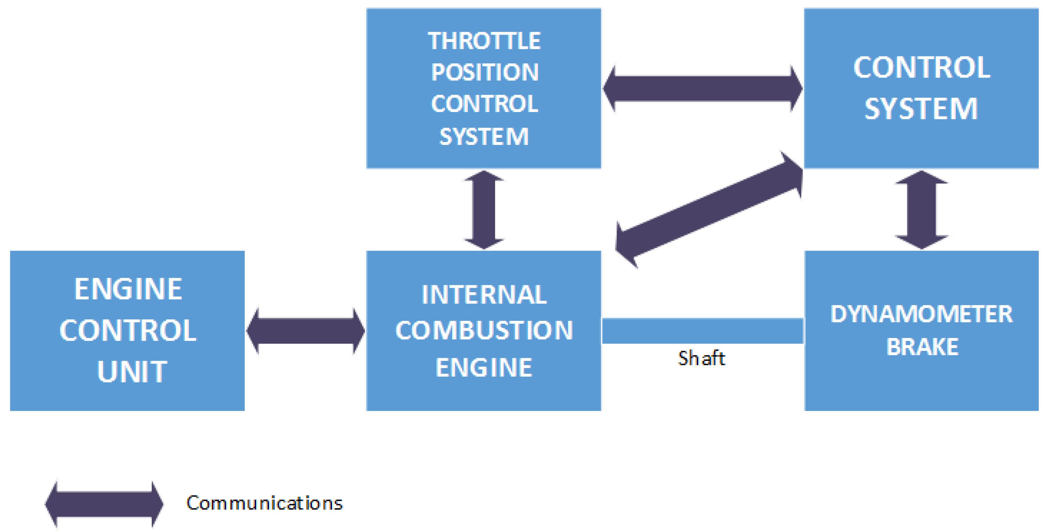
From the point of view of control, Figure 2 shows, as a summary, the structure of the main parts of the plant (test bench) presented in Figure 1. Main components are the engine and the dynamometric brake. Behavior of the system is controlled by the control system. Figure 2 also shows the interactions or communications between all parts of the plant.

4. Plant Parameters

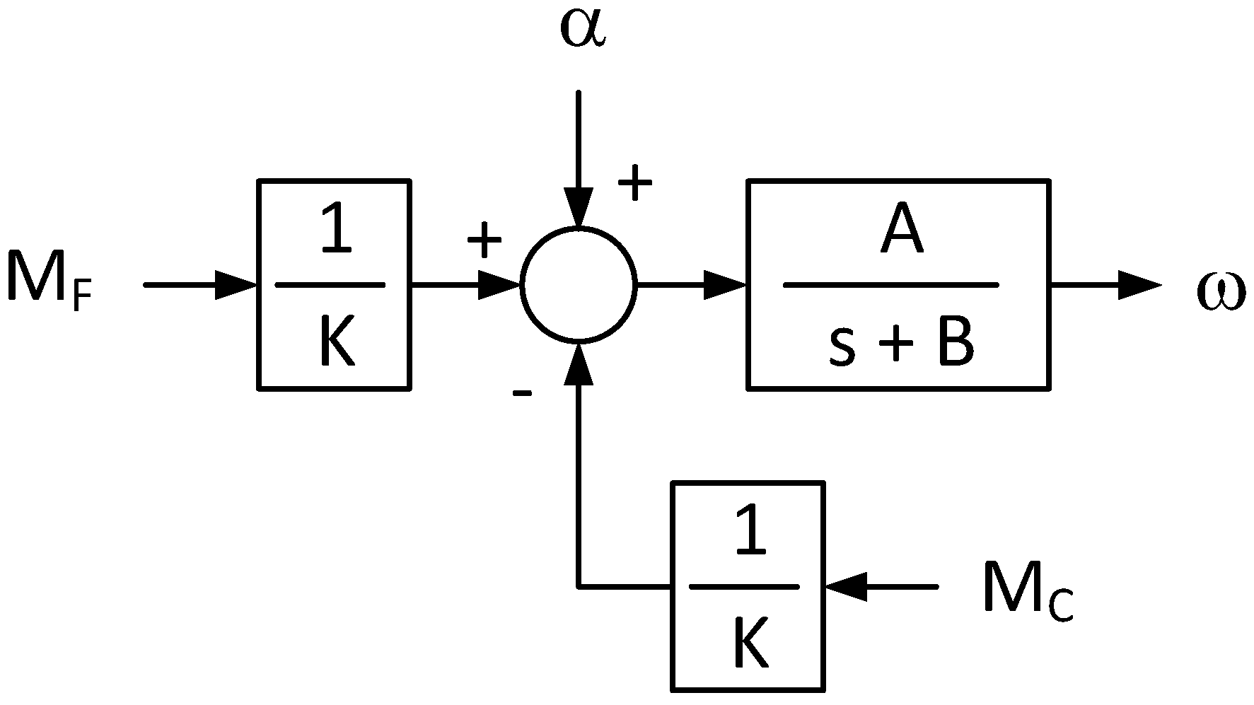
This part shows a summary of the experimental procedure used to obtain the values of the plant parameters. Appendix A shows the theoretical development of the plant mathematical model. This model is presented in Appendix A (Equation (A7)) and defines the dynamical behavior of a system composed by a Diesel engine coupled to a dynamometric brake. Values of parameters A and B are different for each test bench and need to be identified through experimentation. Proposed procedure for parameters identification can be described as follows.

In the test bench control mode $\raisebox{1ex}{$\mathsf{\alpha }$}\!\left/ \!\raisebox{-1ex}{${\mathrm{M}}_{\mathrm{F}}$}\right.$ (control system adjusts the effective torque $\left({\mathrm{M}}_{\mathrm{F}}\right)$ and $\mathsf{\alpha }$ is given as engine input), set demanded effective torque to zero. If ${\mathrm{M}}_{\mathrm{F}}=0$, Equation (A7) yields:

$$\mathsf{\omega }\left(\mathrm{s}\right)=\frac{\widehat{\mathrm{A}}}{\mathrm{s}+\mathrm{B}}$$

(1)

where $\widehat{\mathrm{A}}$:

$$\widehat{\mathrm{A}}=\mathrm{A}\left(\mathsf{\alpha }\left(\mathrm{s}\right)-{\mathsf{\alpha }}_{\mathrm{C}}\left(\mathrm{s}\right)\right)$$

(2)

and:

$${\mathsf{\alpha }}_{\mathrm{C}}\left(\mathrm{s}\right)=\frac{{\mathrm{M}}_{\mathrm{C}}\left(\mathrm{s}\right)}{\mathrm{K}}$$

(3)

where ${\mathsf{\alpha }}_{\mathrm{C}}$is the accelerator position needed to compensate the Coulomb drag.

Equations (1) and (2) show that the engine speed $\left(\mathsf{\omega }\right)$ is related to accelerator position $\left(\mathsf{\alpha }\right)$ and Coulomb drag can be considered as a perturbation input to the system.

Parameters $\mathrm{A}$, $\widehat{\mathrm{A}}$, ${\mathsf{\alpha }}_{\mathrm{C}}$ and $\mathrm{B}$ are obtained studying the time response of the system to a set of $\mathsf{\alpha }$ step inputs [25]. A set of $\widehat{\mathrm{A}}$ and $\mathrm{B}$ parameters are obtained for each experiment and a final $\mathrm{A}$ and $\mathrm{B}$ parameters are obtained for the system from Equations (1) and (2). Figure 3 shows the actual figures for a set of three experiments.

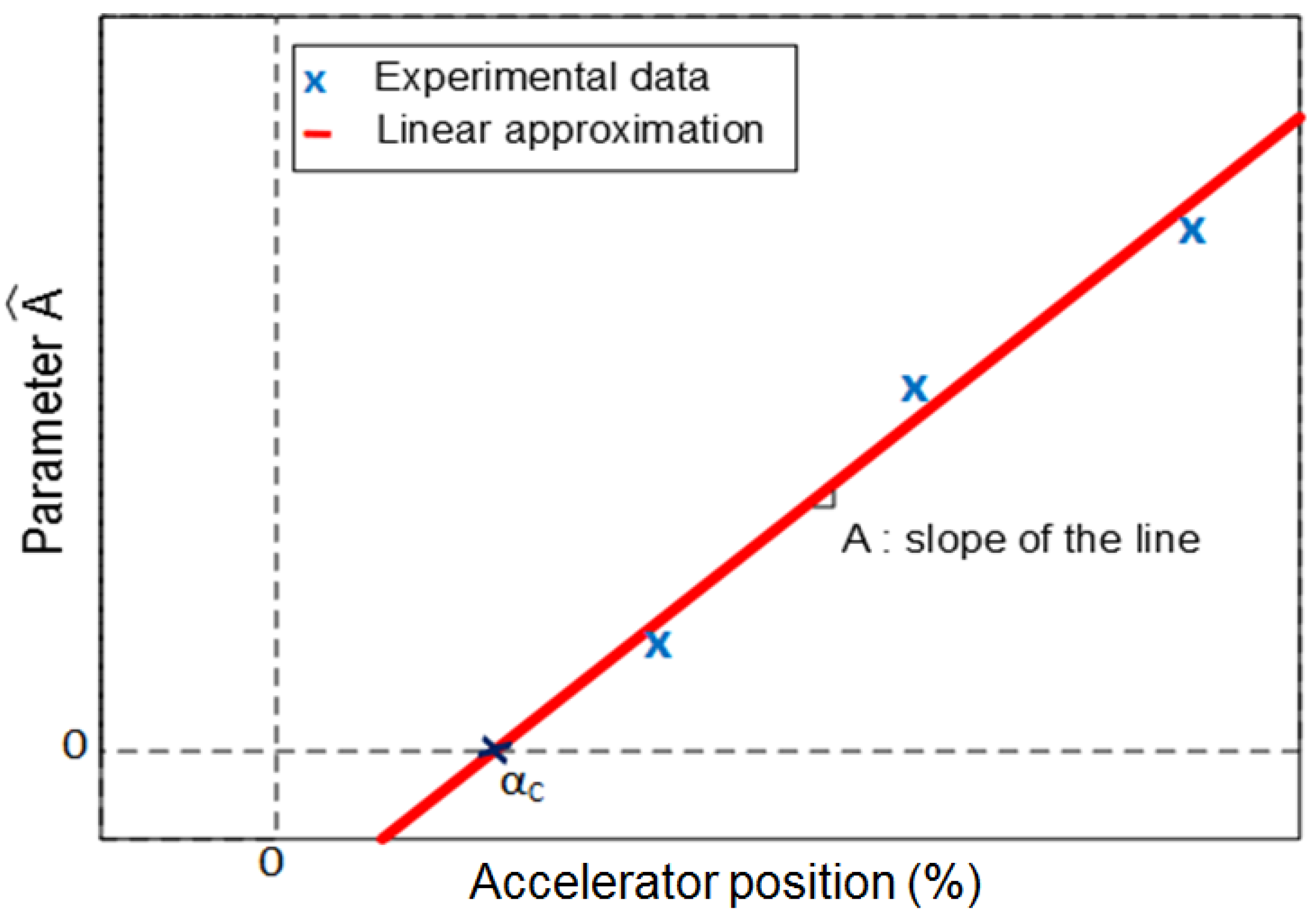
The $\mathrm{A}$ parameter is the slope of the set of $\widehat{\mathrm{A}}$ parameter obtained for each accelerator position. ${\mathsf{\alpha }}_{\mathrm{C}}$ is the zero crossing of the set of experiments while final $\mathrm{B}$ value is obtained as the mean value of the set of B parameters obtained for each experiment. Finally, modelled and experimental results are compared.

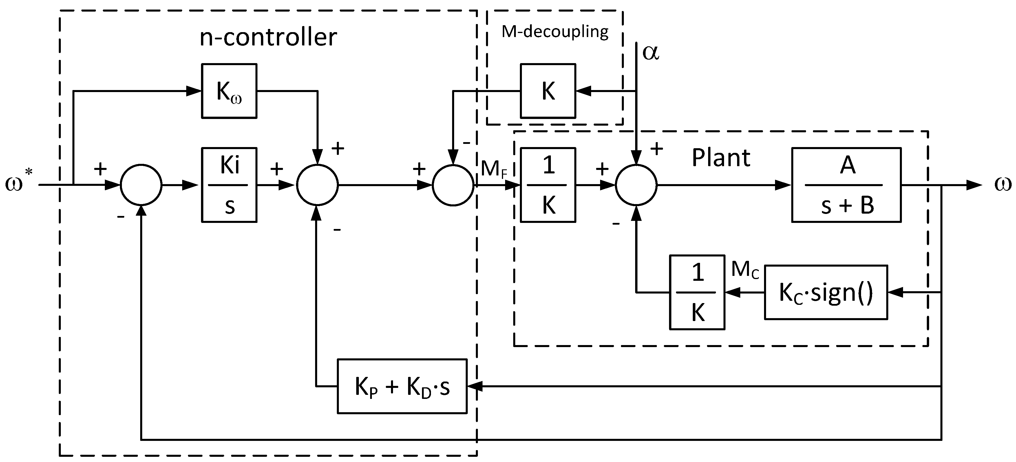
5. Controller Parameters

This part describes how to obtain the values of the test bench control scheme shown in Appendix B. Design requirements are also presented in Appendix B.

5.1. Prefeed

Prefeed gain ${\mathrm{K}}_{\mathsf{\omega }}$ is obtained as the inverse of the plant static gain when effective torque is considered the control variable. Prefeed term equals measured $\mathsf{\omega }\left(\mathrm{t}\right)$ and demanded ${\mathsf{\omega }}^{*}\left(\mathrm{t}\right)$ output in steady state and only if identified plant model fits exactly the actual plant and no perturbations affects the system:

$${\mathrm{K}}_{\mathsf{\omega }}=\frac{\mathrm{K}·\mathrm{B}}{\mathrm{A}}$$

(4)

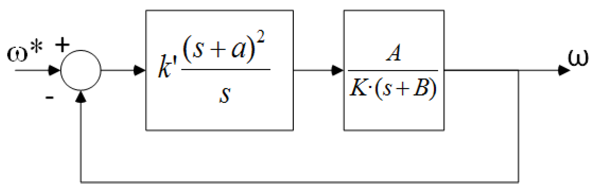
5.2. I-PD Controller

From Appendix B Equation (A8), the transfer function of a classical PID (with the same expression if ${\mathsf{\omega }}^{*}\left(\mathrm{t}\right)=0$, as the I-PD) is:

$$\mathrm{R}\left(\mathrm{s}\right)=\frac{{\mathrm{K}}_{\mathrm{I}}}{\mathrm{s}}+{\mathrm{K}}_{\mathrm{P}}+{\mathrm{K}}_{\mathrm{D}}\mathrm{s}=\frac{{\mathrm{K}}_{\mathrm{I}}+{\mathrm{K}}_{\mathrm{P}}\mathrm{s}+{\mathrm{K}}_{\mathrm{D}}{\mathrm{s}}^2}{\mathrm{s}}$$

(5)

If the same real value is given to both zeros:

$$\mathrm{R}\left(\mathrm{s}\right)={\mathrm{k}}^{\prime }\frac{{\left(\mathrm{s}+\mathrm{a}\right)}^2}{\mathrm{s}}=\frac{{\mathrm{k}}^{\prime }{\mathrm{s}}^2+2{\mathrm{k}}^{\prime }\mathrm{as}+{\mathrm{k}}^{\prime }{\mathrm{a}}^2}{\mathrm{s}}$$

(6)

and the expressions for each parameter are:

$${\mathrm{K}}_{\mathrm{P}}=2{\mathrm{ak}}^{\prime }$$

(7)

$${\mathrm{K}}_{\mathrm{I}}={\mathrm{a}}^2{\mathrm{k}}^{\prime }$$

(8)

$${\mathrm{K}}_{\mathrm{D}}={\mathrm{k}}^{\prime }$$

(9)

From Equations (7)–(9), regulator parameters depends on gain ${\mathrm{k}}^{\prime }$ and double zero $\mathrm{a}$. If only effective torque is considered as plant input, the controlled system is shown in Figure 4, and system characteristic equation yields:

$$1+{\mathrm{k}}^{\prime }\frac{\left({\mathrm{s}}^2+2\mathrm{as}+{\mathrm{a}}^2\right)\mathrm{A}}{\mathrm{Ks}\left(\mathrm{s}+\mathrm{B}\right)}=0$$

(10)

$$\left(\mathrm{K}+{\mathrm{k}}^{\prime }\mathrm{A}\right){\mathrm{s}}^2+\left(\mathrm{KB}+{\mathrm{k}}^{\prime }\mathrm{A}2\mathrm{a}\right)\mathrm{s}+{\mathrm{k}}^{\prime }{\mathrm{Aa}}^2=0$$

(11)

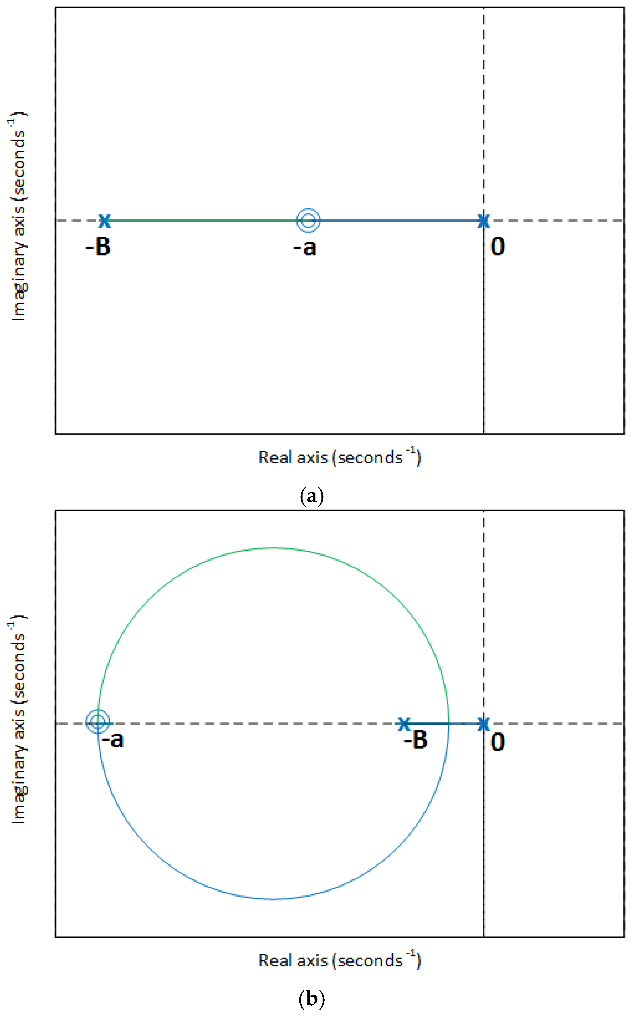
Because no overshooting and the fastest response time are design specifications, closed loop system needs a double real pole. Figure 5 shows a qualitative system root locus depending of the value of “a” where k’ is the variable gain.

If a < B, the only location of the real axis where both poles of the closed loop system can be placed is “a” and this implies an infinite gain k’. For this reason this case will not be considered for further development.

Figure 5b shows the case when a > B. In this case, output from the real axis of root locus branches is the only one valid location for a double pole of the closed loop system. In this case as bigger becomes the “a” value, bigger becomes the control gain and, as a result, bigger becomes the control variable (effective torque) which is not a desirable situation. This last case (a > B) and not enough big “a” will be evaluated in following paragraphs.

Gain k′ can be obtained from Equation (11) as:

$$\mathrm{s}=\frac{-\left(\mathrm{KB}+{\mathrm{k}}^{\prime }\mathrm{A}2\mathrm{a}\right)\pm \sqrt{{\left(\mathrm{KB}+{\mathrm{k}}^{\prime }\mathrm{A}2\mathrm{a}\right)}^2-4\left(\mathrm{K}+{\mathrm{k}}^{\prime }\mathrm{A}\right){\mathrm{k}}^{\prime }{\mathrm{Aa}}^2}}{2\left(\mathrm{K}+{\mathrm{k}}^{\prime }\mathrm{A}\right)}$$

(12)

when:

$${\left(\mathrm{KB}+{\mathrm{k}}^{\prime }\mathrm{A}2\mathrm{a}\right)}^2-4\left(\mathrm{K}+{\mathrm{k}}^{\prime }\mathrm{A}\right){\mathrm{k}}^{\prime }{\mathrm{Aa}}^2=0$$

(13)

or:

$${\mathrm{K}}^2{\mathrm{B}}^2+4\mathrm{KAa}\left(\mathrm{B}-\mathrm{a}\right){\mathrm{k}}^{\prime }=0$$

(14)

and finally:

$${\mathrm{k}}^{\prime }=-\frac{{\mathrm{KB}}^2}{4\mathrm{Aa}\left(\mathrm{B}-\mathrm{a}\right)}$$

(15)

that, when a > B becomes:

$${\mathrm{k}}^{\prime }=\frac{{\mathrm{KB}}^2}{4\mathrm{Aa}\left(\mathrm{a}-\mathrm{B}\right)}$$

(16)

5.3. Decoupling Gain

The decoupling gain K is used to decouple (cancel) the effect of the $\mathsf{\alpha }$ in control variable (effective torque). As can be seen in Appendix A:

$$\mathrm{K}=\mathrm{JA}$$

(17)

where J is the inertia of the set composed by the engine + dynamometer, from manufacturer data, and A is obtained as described in previous paragraphs.

6. Results and Discussion

6.1. Results from the Plant Simulation and Its Experimental Validation

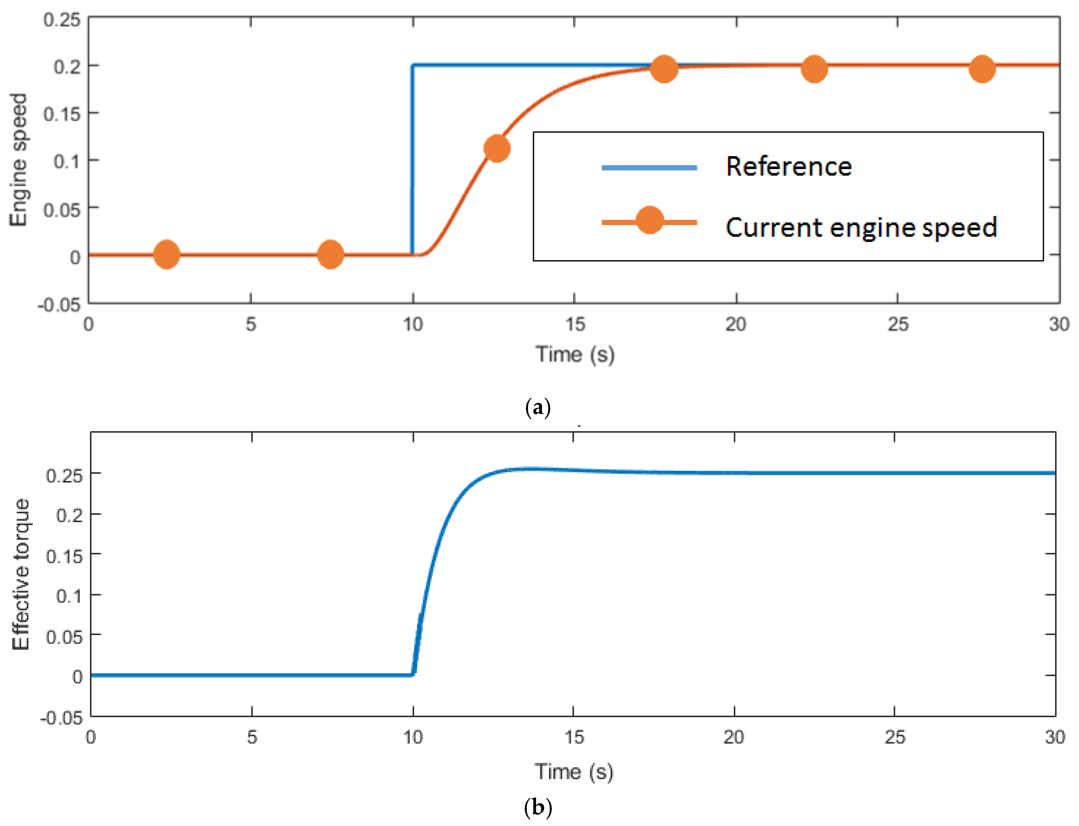
Previously described methodology has been applied to a theoretical system considering a normalized plant. This means parameters A, B and K equals 1 and every variable in the model ranges from 0 to 1. Engine speed demand $\left({\mathsf{\omega }}^{*}\right)$ and accelerator position $\left(\mathsf{\alpha }\right)$ have been taken as step signals with arbitrary final value (${\mathsf{\omega }}^{*}=0.2$ and $\mathsf{\alpha }=0.5$). Also an arbitrary value has been chosen for Coulomb drag (${\mathrm{M}}_{\mathrm{C}}=0.05$). To avoid step changes in effective torque, a first order filter has been used to smooth step shape of input signals ${\mathsf{\omega }}^{*}$ and $\mathsf{\alpha }$.

Control law parameters (${\mathrm{K}}_{\mathsf{\omega }}$, ${\mathrm{K}}_{\mathrm{P}}$, ${\mathrm{K}}_{\mathrm{I}}$, ${\mathrm{K}}_{\mathrm{D}}$) have been obtained from Equations (4), (7)–(9) and (17) when a > B. As an example, setting $\mathrm{a}=1.5\mathrm{B}$ gives values such as ${\mathrm{K}}_{\mathrm{P}}=1$, ${\mathrm{K}}_{\mathrm{I}}=0.749$, ${\mathrm{K}}_{\mathrm{D}}=0.333$. Figure 6 shows simulated engine speed and effective torque obtained with previous values.

Experimental validation of the presented methodology has been carried out in facilities presented in Figure 1. This installation is operative in the laboratory managed by the Energy and Environmental Processes Investigation Group (www.grupogpem.com).

The procedure followed to obtain the experimental results shown in next paragraphs has been as described in previous sections. Plant parameters A and B (Equations (2) and (3)) have been identified from several sets of experimental data.

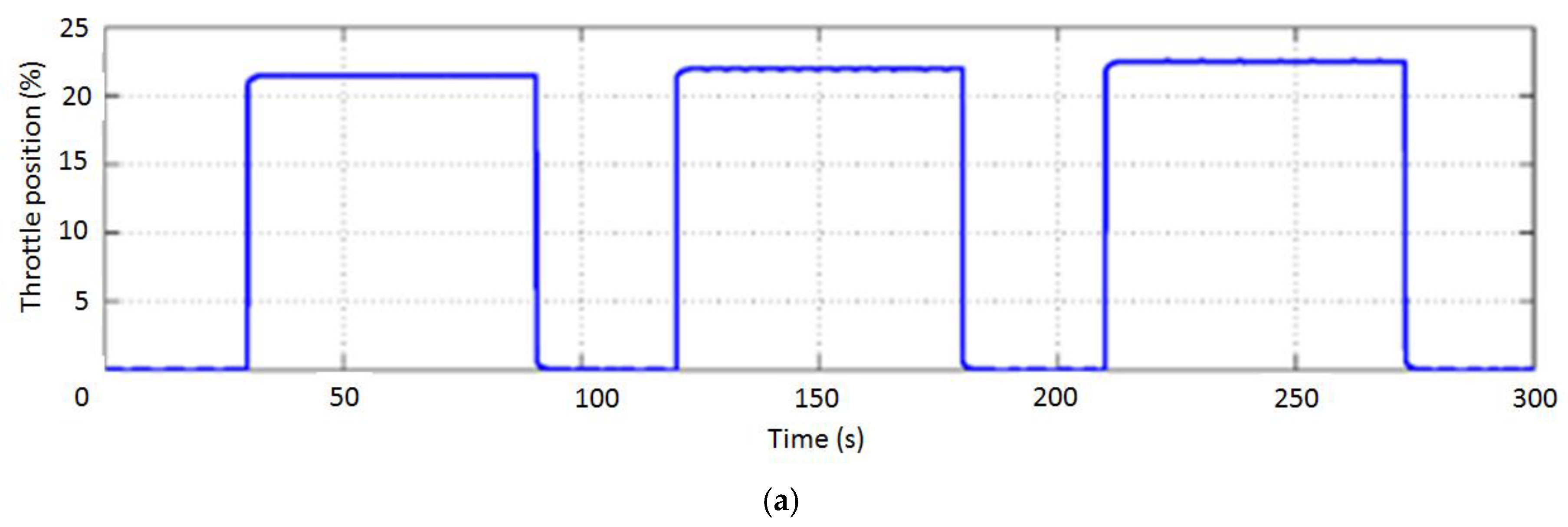
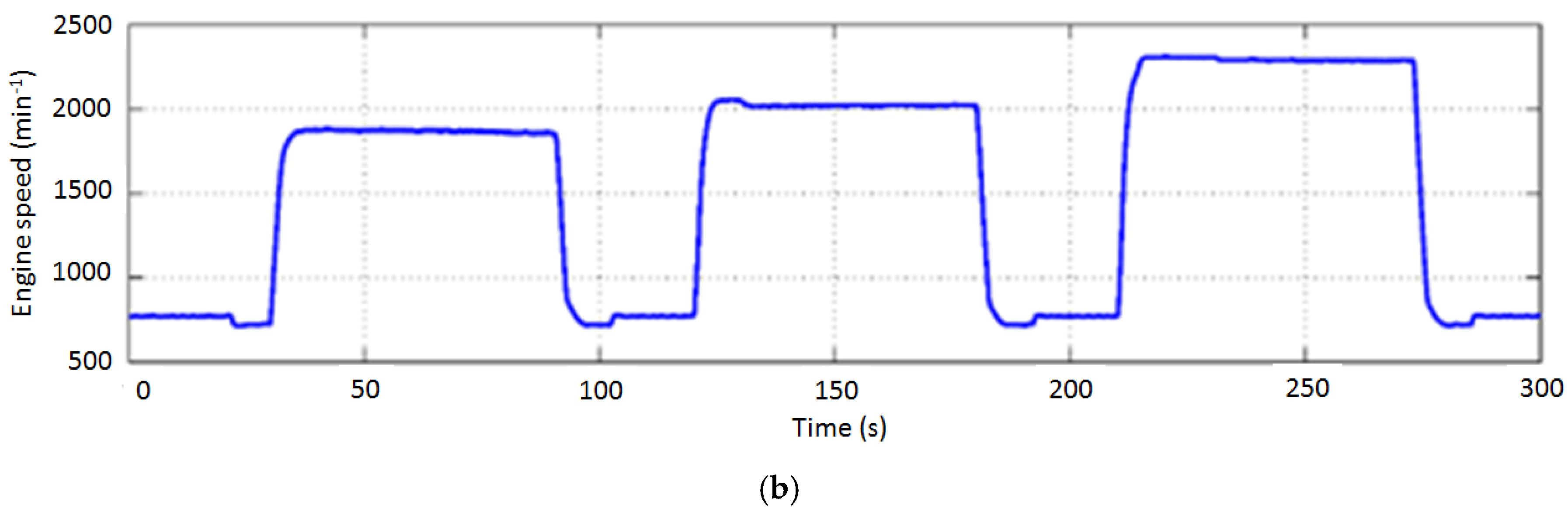
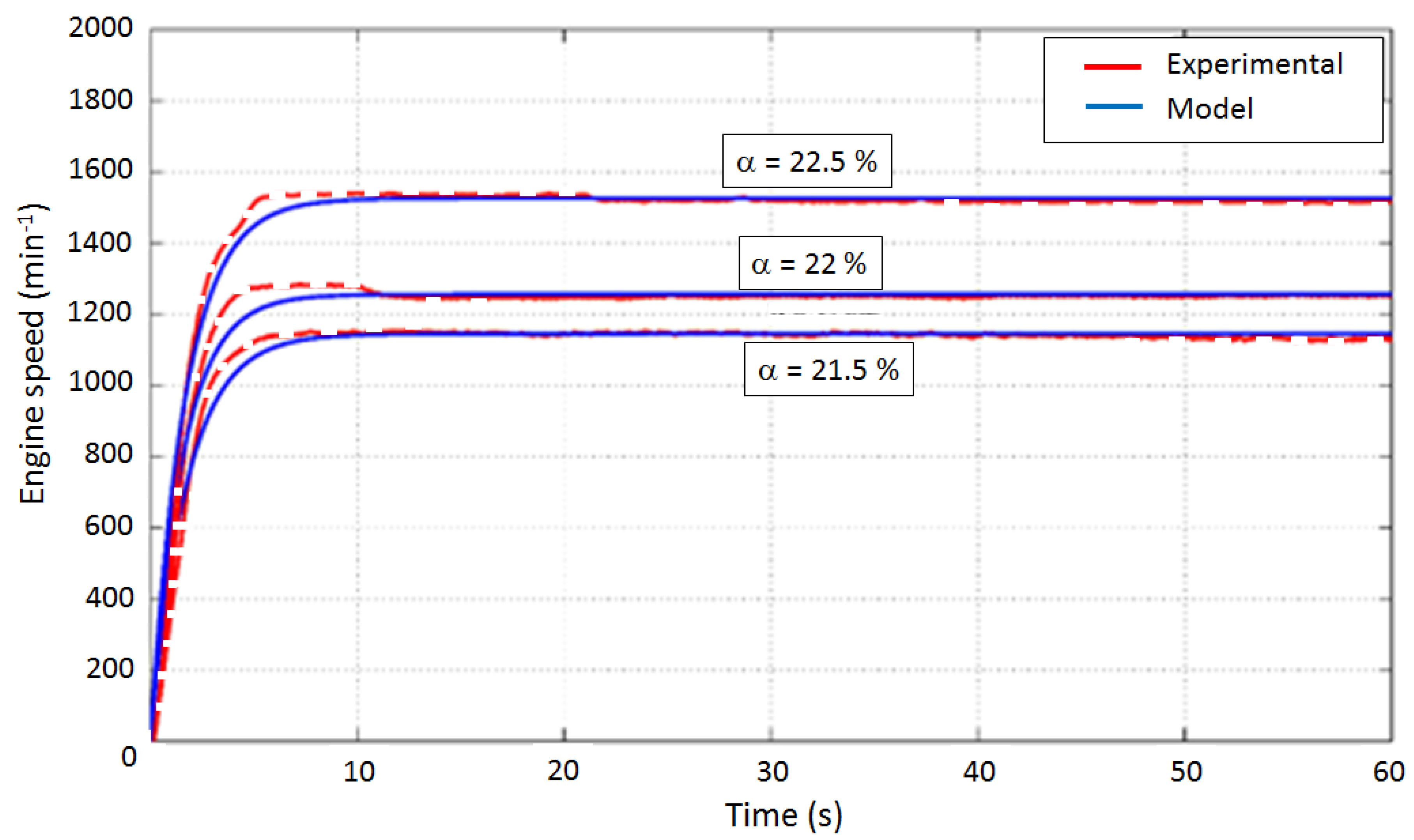
First, $\widehat{\mathrm{A}}$ and $\mathrm{B}$ were obtained using time domain experiments. System response to a pulse sequence (see Figure 7) was evaluated. Values of 21.5, 22 and 22.5 % of accelerator position were tested. These tests were performed without load (effective torque = 0 Nm), i.e., the opposition torque generated by the dynamometric brake was zero. The minimum accelerator position to compensate the Coulomb friction is 19.06% (as Section 5.1 shows). On the other hand, the maximum accelerator position tested without load (null effective torque) was 23% because from this value the engine speed increases a lot and exceeds the torque limit of the test bench. Elapsed time for these values was fitted in 60 s while time between values was fitted in 30 s and the engine was working in idle condition.

Numerical fitting procedure proposed by Levenberg-Marquardt [26,27] has been used to obtain $\widehat{\mathrm{A}}$ and $\mathrm{B}$ values.

Table 3. $\widehat{\mathrm{A}}$ and $\mathrm{B}$ values for each accelerator position.

Accelerator Position (%)	$\widehat{\mathbf{A}}$	B
21.5	650.40	0.568
22.0	810.01	0.645
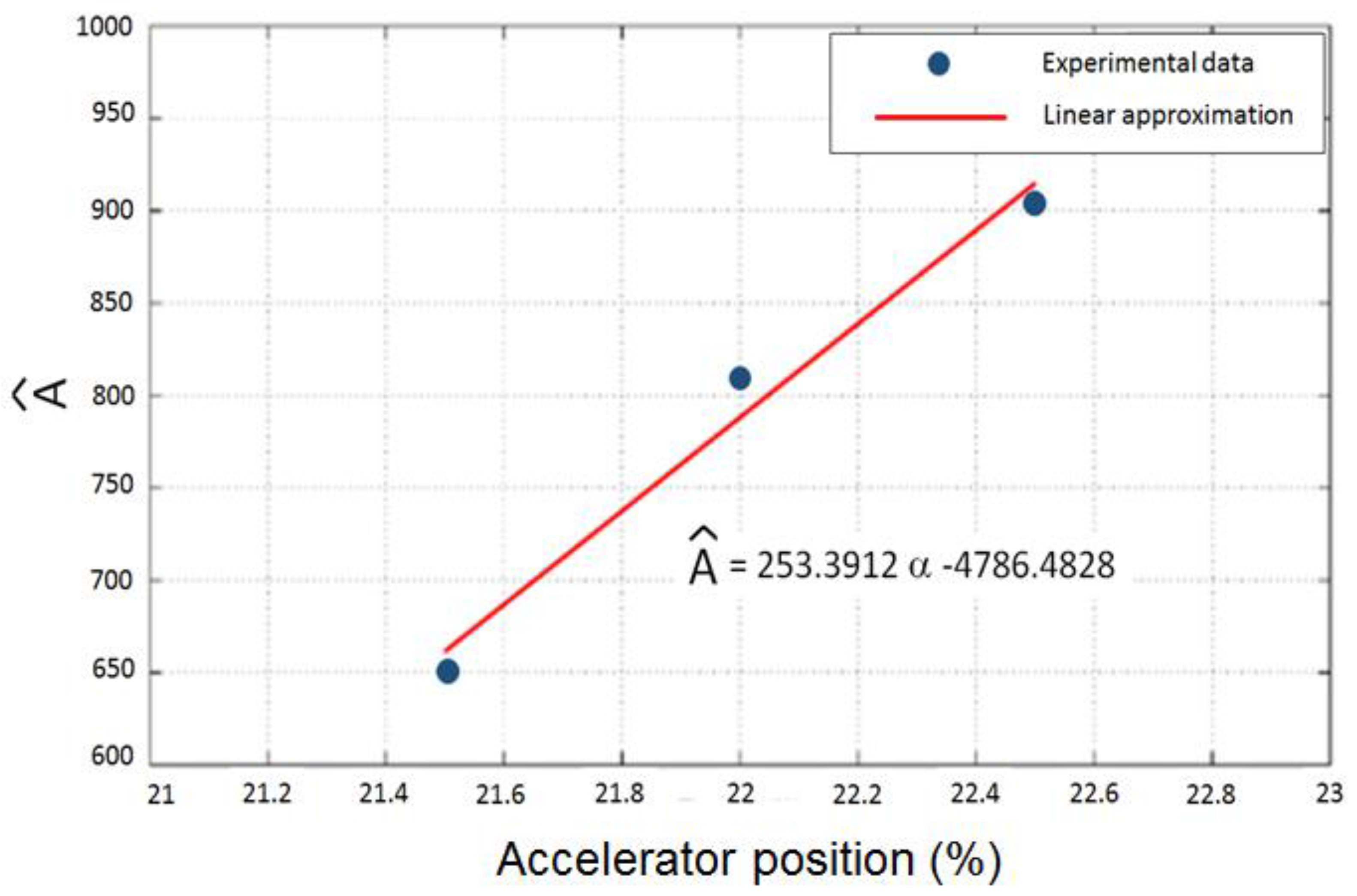
22.5	903.88	0.592

shows the obtained values for each accelerator position.

New values of $\widehat{\mathrm{A}}$ and $\mathrm{B}$ are obtained for each accelerator position. “$\mathrm{A}$” value is obtained as the slope of the line relating $\widehat{\mathrm{A}}$ and accelerator position and ${\mathsf{\alpha }}_{\mathrm{C}}$ is the zero crossing of the line, as stated in previous section. Figure 8 shows the values obtained for $\mathrm{A}$ and ${\mathsf{\alpha }}_{\mathrm{C}}$ in experiments. B is obtained as the mean value of B from Table 3.

Finally, the values for the setup were: $\mathrm{A}=250.45$, $\mathrm{B}=0.56$ and ${\mathsf{\alpha }}_{\mathrm{C}}=19.06\%$. Figure 9 shows the response of both the actual system and the identified model.

6.2. Results from the Engine Tested before and after the Test Bench Tuning

Test bench control electronics is an X-act brake controller and it is able to implement the control laws proposed in this work. Control parameters (K, K_ω, K_P, K_I, K_D) were obtained from Equations (4), (7)–(9), (16) and (17). Parameters A and B were obtained during the plant identification process and value J was obtained from the engine and brake manufacturers. Finally, the definitive data set for the test bench tuning has been: $\mathrm{J}=0.4 {\mathrm{Kgm}}^2$ [24], $\mathrm{K}=100.18$, ${\mathrm{K}}_{\mathsf{\omega }}=0.22$, ${\mathrm{K}}_{\mathrm{P}}=0.22$, ${\mathrm{K}}_{\mathrm{I}}=0.09$, ${\mathrm{K}}_{\mathrm{D}}=0.13$. These values have to be intended as the first step of an experimental tuning, but rather close to final ones. The previous values of the controller parameters (manufacturing calibration) were: $\mathrm{K}=20$, ${\mathrm{K}}_{\mathsf{\omega }}=0.22$, ${\mathrm{K}}_{\mathrm{P}}=0.22$, ${\mathrm{K}}_{\mathrm{I}}=0.09$, ${\mathrm{K}}_{\mathrm{D}}=0.01$.

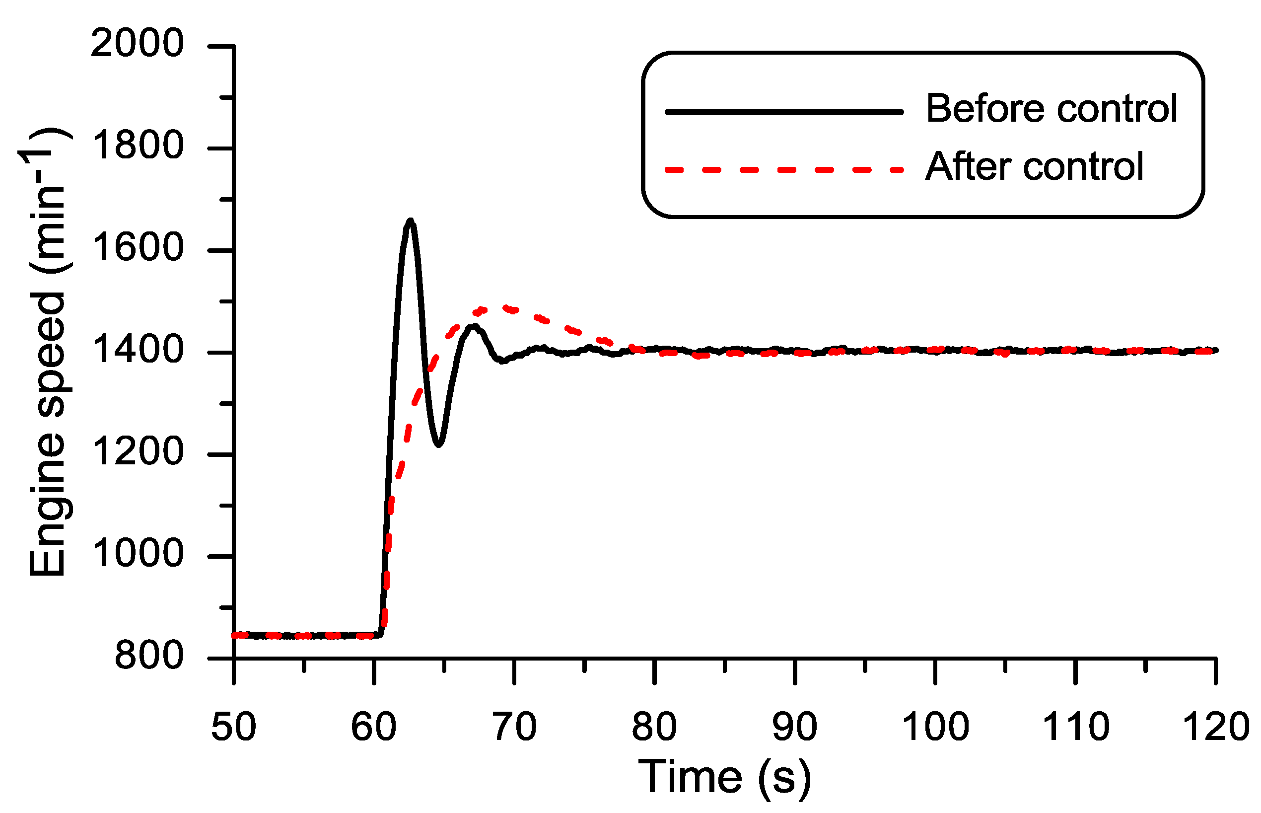
For demonstrating the effect of the test bench tuning on performance and emissions, a transient test from idle to an engine speed demand of 1400 min⁻¹ and accelerator position from 0 to ~4% was carried out.

These actions produced the time evolutions of the engine speed before and after the test bench tuning presented in Figure 10. As can be seen, before tuning, the test bench control settings produced a great oscillation of the engine speed at the end of the transient process tested. After the test bench tuning, the engine speed overshoot is less than 10%.

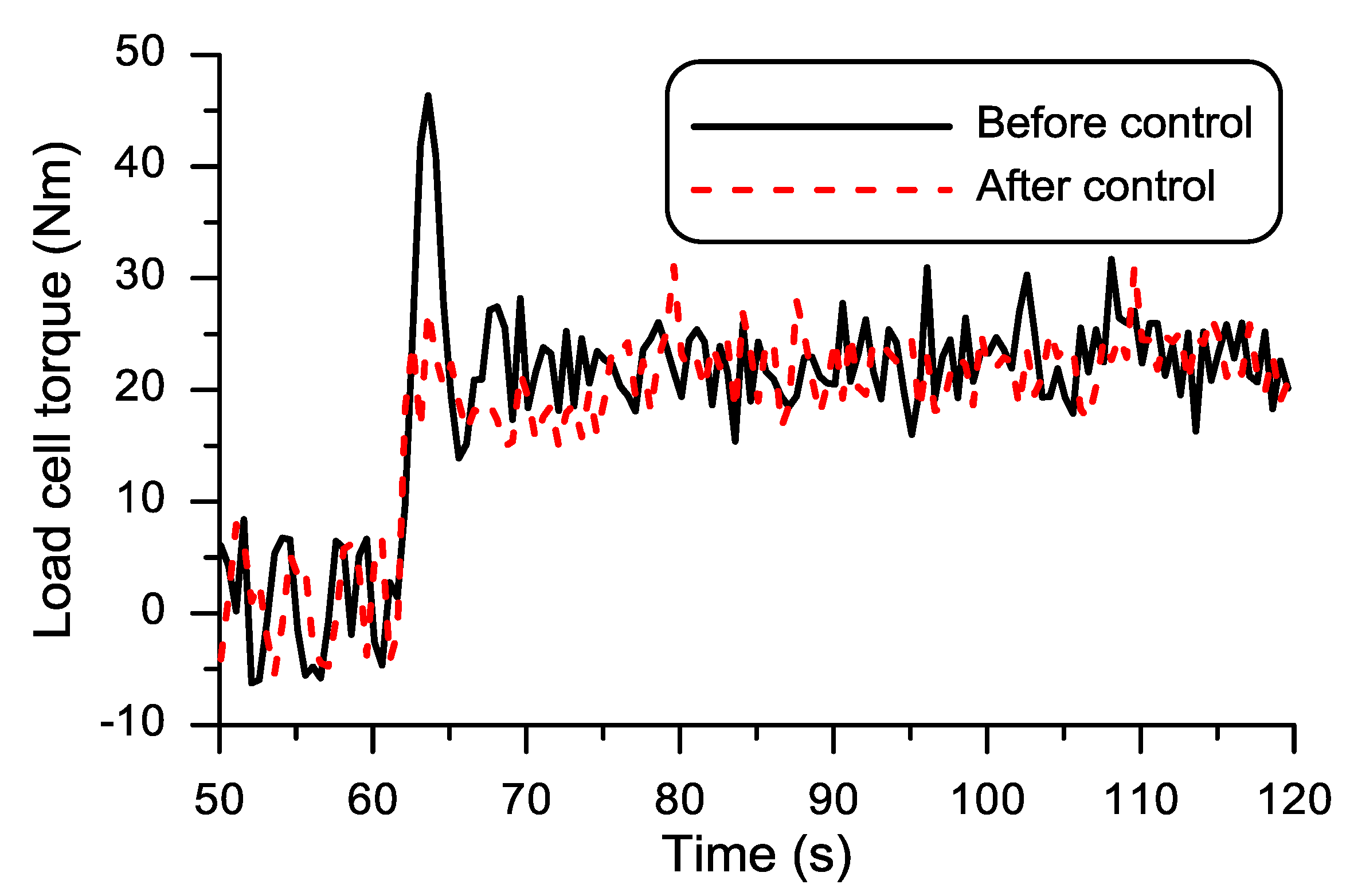
The evolution of the engine speed shown in Figure 10 can be explained by the evolution of the load cell torque (control effort) as consequence of the engine torque and the inertia of the rotating masses (axe and dyno) as Figure 11 shows. These torque oscillations could damage the coupling shaft between the engine and the dynamometer brake.

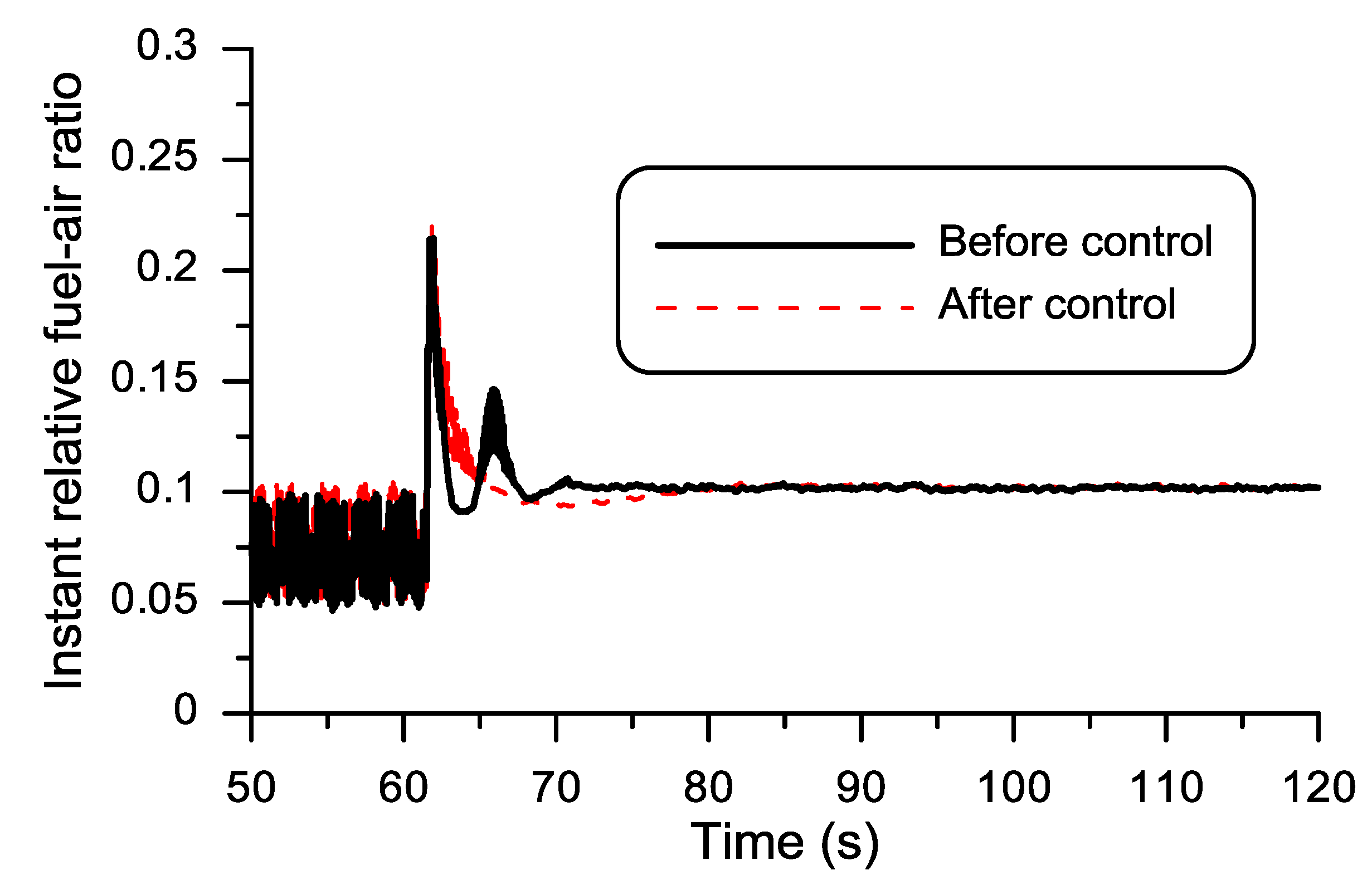
As Figure 11 shows, before the test bench tuning, a great peak of the load cell torque is produced by the peak of relative fuel-air ratio (great fuel-air mixture enrichment produced by the engine) trying to reach the desirable engine speed limit. Figure 12 shows the time evolution of the relative fuel-air ratio.

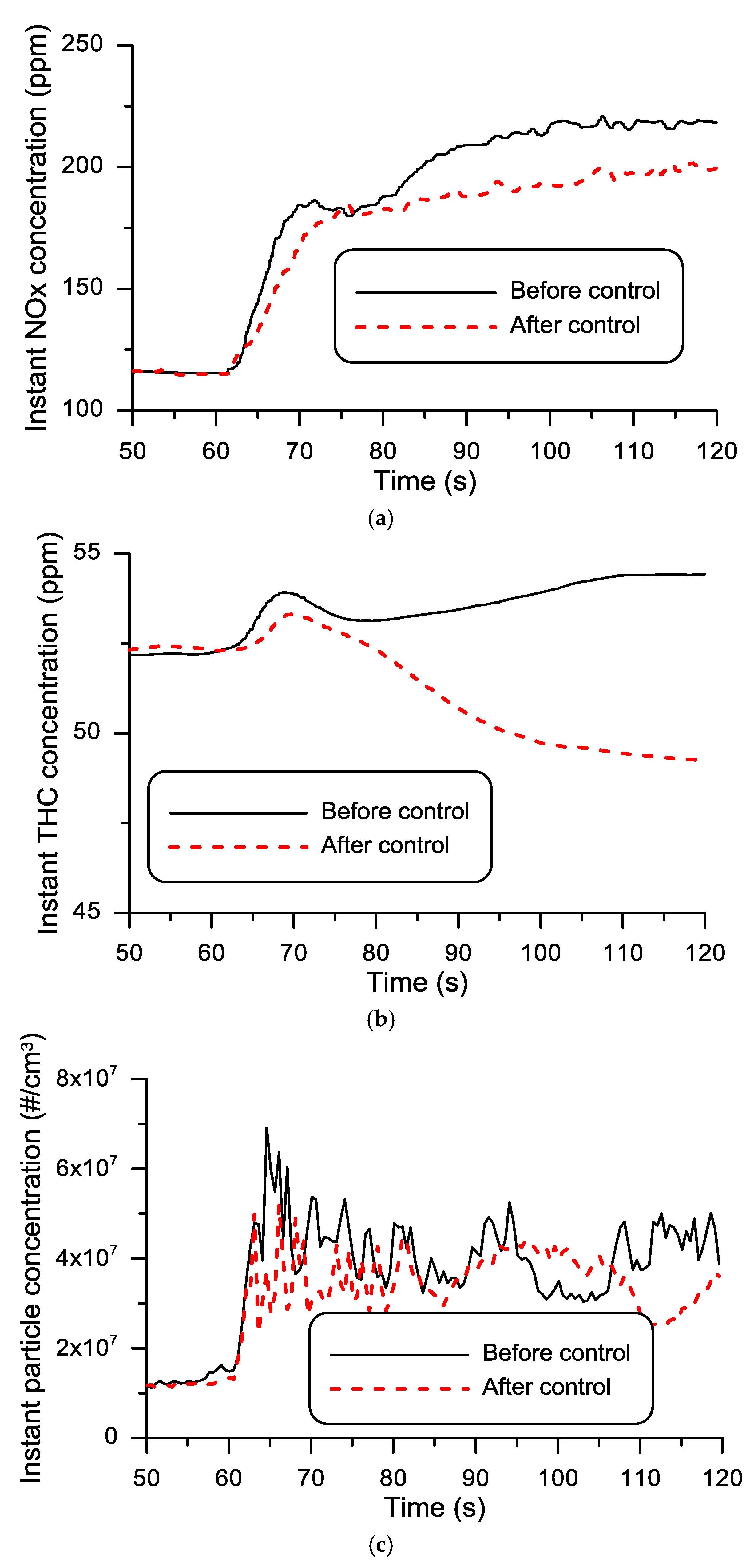
The great oscillations of relative fuel-air ratio produced negative consequences not only on both the engine speed and torque but also on pollutant emissions. Figure 13 shows the time evolution of nitrogen oxides (NO_x), total hydrocarbons (THC) and particle concentrations before and after the test bench tuning.

As can be seen in Figure 13, values of NO_x and THC concentrations show the effect of both test bench tunings even when the time response of the gas analyzers is not enough fast as the tested process requires. Particle concentrations is coherent with the values of the relative fuel-air ratios registered. By the other hand, after an increase of the accelerator position from engine idle operation to an operating mode under external load, initially, the effectiveness of the Diesel Oxidation Catalyst (DOC) is lower because the initial temperature is lower than the light off temperature of the DOC. When the light off temperature increases then it begins the pollutant reduction. In this work, in both cases, the data recording finished before reaching the steady state thermal condition of the DOC.

Despite the fact the engine received the same accelerator position order during the transient process tested, the test bench tuning imposes very different behavior on the engine, particularly on the relative fuel-air ratio and, in consequence, affecting pollutant emissions.

7. Conclusions

This work has demonstrated the importance of using a suitable control law and adjusting the controller parameters in a reciprocating internal combustion engine test bench. Some engine performance profiles (engine speed, engine torque and relative fuel air ratio) and pollutant emissions (nitrogen oxides, hydrocarbons concentrations and number of particles emitted) have been compared under two different situations: unadjusted and adjusted control system. Great oscillations of relative fuel-air ratio disappear in the transient process by using an adjusted control system. This implies that the overshooting in the demanded engine speed and torque is reduced more than fifty percent. Consequently, pollutant emissions are also reduced.

A methodology has been proposed to adjust the control system, even for inexperienced professionals in control engineering in charge of this type of equipment. This methodology covers from experimental plant modelling to control parameters determination and experimental validation.