The Amalgamation of SVR and ANFIS Models with Synchronized Phasor Measurements for On-Line Voltage Stability Assessment

1
Department of Electrical Engineering, University of Ferhat Abbas Setif 1, Setif 19000, Algeria
2
Faculty of Electrical Engineering, Universiti Teknologi MARA, Shah Alam 40450, Malaysia
*
Author to whom correspondence should be addressed.
Energies 2017, 10(11), 1693; https://doi.org/10.3390/en10111693
Submission received: 3 September 2017
/
Revised: 17 October 2017
/
Accepted: 18 October 2017
/
Published: 25 October 2017
(This article belongs to the Section F: Electrical Engineering)
Abstract
:This paper presents the application of support vector regression (SVR) and adaptive neuro-fuzzy inference system (ANFIS) models that are amalgamated with synchronized phasor measurements for on-line voltage stability assessment. As the performance of SVR model extremely depends on the good selection of its parameters, the recently developed ant lion optimizer (ALO) is adapted to seek for the SVR’s optimal parameters. In particular, the input vector of ALO-SVR and ANFIS soft computing models is provided in the form of voltage magnitudes provided by the phasor measurement units (PMUs). In order to investigate the effectiveness of ALO-SVR and ANFIS models towards performing the on-line voltage stability assessment, in-depth analyses on the results have been carried out on the IEEE 30-bus and IEEE 118-bus test systems considering different topologies and operating conditions. Two statistical performance criteria of root mean square error (RMSE) and correlation coefficient (R) were considered as metrics to further assess both of the modeling performances in contrast with the power flow equations. The results have demonstrated that the ALO-SVR model is able to predict the voltage stability margin with greater accuracy compared to the ANFIS model.
1. Introduction
In recent years, the voltage instability problem has become an imperative research area in the field of power system due to the advent of competitive electricity market inflicting towards an intense and complex planning that shove the system to operate near to their stability limits [1]. In such situations, and for better operation of the system, the voltage stability margins (VSM) and control actions must be determined in an on-line manner. Hence, it is indispensable that the measurement, the estimation, and the analysis be attained during a short period of time. Traditionally, the voltage phasors i.e., voltage magnitudes and angles at all system buses are provided by supervisory control and data acquisition (SCADA) typically every few minutes [2]. Nowadays, phasor measurement unit (PMU) is employed in many countries to enhance the security, reliability, and the efficient monitoring of the power system [3]. When compared to the slow nature of SCADA, PMU devices are able to provide the synchronized measurement data (voltages and currents), with great accuracy and 100 times faster than SCADA system [2]. However, due to the high cost of the PMU devices, it is neither economical nor possible to install these units on the entire power system buses [4]. On the other hand, the numerous tools that have been developed and introduced by the researchers to conduct a comprehensive analysis on the voltage stability assessment, such as P–V and Q–V curves, continuation power flow and voltage stability indices [5,6,7] have the scarcity to be used in a real-time or on-line operation, as they are computationally time-consuming due to its reliant on a complex mathematical modeling of a power system.
The aforementioned impediments of PMUs installation costs and enormous computational requirements of the traditional methods of voltage stability analysis could be resolved by utilizing the advanced biological computation of artificial intelligence (AI) techniques, such as the artificial neural network (ANN), adaptive neuro-fuzzy inference system (ANFIS), and support vector machines (SVM).
Several ANN architectures have been implemented in on-line voltage stability assessment. Debbie et al. [8] presented an ANN-based method for on-line assessment of the voltage stability. Chakrabarti [9] proposed a new methodology for on-line voltage stability monitoring using multi-layered perceptron neural network and a regression-based method of selecting features for training the network. Jayasankar et al. [10] used a single ANN trained by the back-propagation algorithm to evaluate the voltage stability of power system incorporating flexible AC transmission system (FACTS) devices. Further improvement of ANN performance in an on-line monitoring of voltage stability has been realized by reducing the input data into an optimal size using Z-score based algorithm [11]. It is worthwhile to notify that the load active and reactive powers are generally used as the input features for the ANN [12]. The application of ANN-based radial basis function (RBF) for on-line voltage stability assessment has been performed by several researchers [13,14,15,16]. The application of self-organizing Kohonen-neural network (KNN) for fast indication and visualization of voltage stability has been conferred [17]. Chakraborty et al. [18] incorporated a self-organizing feature map (SOFM) with RBF network for detection and classification of power system voltage instability. Duraipandy et al. [19] proposed the use of extreme learning machine (ELM) technique for on-line voltage stability assessment with multiple contingencies. Albeit, the ANN has gained considerable attention from researchers in lately as a tool for on-line voltage stability assessment, it has several limitations particularly with respect to a relatively long time required for the training process as well as the problem of sticking at local minima [20].
Other techniques such as decision tree (DT) and multilinear regression models (MLRM) have been also applied to assess power system voltage stability [21,22,23,24]. Zheng et al. [21] proposed the use of DT for fast and accurate evaluation of voltage stability based on PMUs data. Li and Wu [22] employed the gathered voltage phase angles from PMUs to enhance DT’s identification precision. In [23], a novel on-line voltage security assessment technique based on wide-area measurements, adaptive boosting technique, and DT algorithm has been developed. Bruno and Venkataramana [24] proposed a new methodology to estimate the VSM of power system using statistical MLRM and reactive power reserves.
In the last decade, the use of ANFIS and SVR models has attracted much attention to the researchers since these techniques have several advantages and have been successfully applied in different engineering areas. The ANFIS model is a well-developed fuzzy inference system that takes into account the important elements of fuzzy logic and neural network. The prelude utilization of ANFIS has been explored to perform a comprehensive risk assessment of voltage collapse [20]. The model is constructed in conjunction with the input information of voltage stability indices termed as the VOltage STAbility (VOSTA), while the output was the megawatt (MW) distance of the current operating point from the stability limit demarcated for voltage collapse analysis. Torres et al. [25], uses the subtractive clustering (SC) and ANFIS methods to estimate the loadability margin by means of various voltage stability indices that have been chosen as the inputs. More recently, the Kohonen-self-organizing map is employed to cluster the real and reactive loads to reduce the input features of ANFIS to compute the loadability margin of a power system incorporating FACTS devices [26].
Recently, the voltage instability condition of power system has been assessed by imposing SVM [27], which is a powerful machine learning technique that based on statistical learning theory. However, its application in voltage stability assessment is still in a small volume. Nevertheless, SVM has become a very interesting topic due to its successful application towards classification and regression tasks in other fields of research [28]. Cortés et al. [29] successfully employed every single SVM that was trained to classify the state of a system either it is secure, alert, or emergency. The final classification representing a system security assessment is obtained from the combination of each classifier output undertaken by using the Bayesian rule. This approach has been implemented that is relatively similar to the proposed multi-class SVM used for security assessment that has been discussed in [30]. In the proposed approach, there are four different statuses of system security: normal, alert, emergency_1, and emergency_2 for system splitting statuses that have been used to classify the system security. Further improvement of multi-class SVM has been undertaken by consolidating the pattern recognition approach for security assessment [31]. Support vector regression (SVR) is an extended version of SVM that has been used to predict the VSM of a power system incorporating flexible AC transmission system (FACTS) devices [32]. On the overleaf, a new methodology for on-line prediction of VSM has been introduced by deploying the SVR trained by taking into account the input information of real and reactive power load at all of the buses [28].
Notwithstanding that SVR is an efficient method to solve the nonlinear regression problems, there are no general guidelines to define their parameters, which becomes an impediment to the breadth of the use of SVR in manufacturing applications and scientific research. Inappropriate chosen values of SVR parameters lead to over-fitting or under-fitting problems, and various parameter settings can also lead to considerable differences in performance [33]. Traditionally, experience-based trial and error [34], grid search algorithm [35], and gradient descent algorithm [36] are the most applied techniques to select the SVR parameters. Convergence to local minima point, computational complexity, and height computational time requirement are the major drawbacks of these conventional methods [37]. With the development of meta-heuristic optimization algorithms, some of them have been adopted to determine the SVR parameters, such as genetic algorithm (GA) [38] and particle swarm optimization (PSO) [39]. However, the performance of these methods is imperfect, the GA encloses a sequence of processes, i.e., coding, selection, crossover, and mutation, which could affect the speed and the precision of this optimization technique. In the same way, the effectiveness of the PSO is influenced by the particle’s multiple parameters [40].
This paper presents the application of SVR and ANFIS in predicting the VSM with regards to the input data of voltage magnitudes attained from PMUs. As the prediction capability of SVR model tremendously depends on the good selection of its parameters, the recently developed ant lion optimization (ALO) algorithm was employed to determine the optimal parameters of SVR model. Thereafter, the developed ALO-SVR model has been applied to assess the voltage stability and was compared to the ANFIS model. The effectiveness of the proposed approach is verified using the IEEE 30-bus and 118-bus test systems.
2. Voltage Stability Assessment
It is perspicuous that a power system operating at the pinnacle of the unstable condition is conspicuously referring to the voltage magnitude approaching to its limit and it is presented by the voltage stability indices. Many voltage stability indices have been used to evaluate the voltage instability condition [7,41,42,43]. In this work, the voltage stability index (VSI) is taken as an indicator of voltage stability. The major advantage of this index is that the mathematical formulation is derived considering all of the system margins including active, reactive, and apparent power margins [44]. The derivation of VSI formulation is originated from a 2-bus system, where the active (Pr) and reactive (Qr) powers at the receiving bus can be given by Equations (1) and (2), respectively., The voltage at Vr, resulted from combining these equations with eliminating δ, can be expressed by Equation (3).
where Vs and Vr are the voltages at the sending and receiving buses, respectively; R and X are the line resistance and the line reactance, respectively.
The maximum transferable power, Smax, through the line is attained as the internal root phrase equals to zero [43]. There is only one solution for Vs and Vr is at the collapse point.
The maximum transferred active power Pmax, the maximum transferred reactive power Qmax and the maximum transferred power Smax can be expressed by Equations (4)–(6), respectively:
where θ is the load power angle, .
These Equations can be simplified by assuming high X to R ratio.
Therefore, according to these relations, the total on-line VSI can be calculated as [44]:
A small value of VSI indicates that the voltage magnitude at the load bus is close to its collapse point. Once the voltage magnitude at a load bus has reached its collapse point, and consequently the VSI is equal to zero and vice-versa.
3. A Brief Theoretical Background of SVR and ANFIS Models
This section explicates the theoretical background of SVR and ANFIS models with concise mathematical equations representing the relationship among all variables.
3.1. SVR Model
Support vector machine (SVM) was developed by Vapnik [27] on 1995. It has become a very important computational tool due to its successful application in classification and regression tasks [28]. SVR is an extended version of SVM that was developed to estimate regression functions and it has received an increasing attention in the estimation of nonlinear problems. The SVR is based on the mapping of the original data x nonlinearly into a higher dimensional feature space. In order to illustrate the concept of SVR, one should consider a regression function F, which is estimated based on a given training data, {(xi, yi) i = 1, 2, …, n}, where xi are the inputs, yi are the outputs, and n is the number of patterns. SVR estimates the target values by using the linear equation as follows [45].
where F is the output, w is the weight vector, b is the constant (bias), and ϕ(x) is the high dimensional real input vector. The ε-insensitive loss function is used to represent the deviation between the actual values and the regression function. This deviation can be treated as a tube spanning around the regression function. Any points outside of the tube are viewed as training errors. The coefficients w and b purporting as the support vector weight and bias calculated by minimizing the risk function as given below.
where
In Equation (12), the first term is the ε-insensitive loss function. Moreover, the second term is used to estimate the function flatness. Accordingly, parameter C is used to specify the trade-off between function complexity and losses (penalty parameter). Two positive slack variables ξ and ξ* which are equal to zero if the data points are within the ε-tube. Then, Equation (12) can be transformed into the following constrained form [45].
The above problem can be solved by adding Lagrangian multipliers and considering the case of non-linear regression by including the mapping to the feature space:
where and are the Lagrange multipliers. The vector inner-product (ϕ(xi)·ϕ(xj)) can be replaced by the kernel function K(xi,xj). Hence, the Equation (16) becomes:
The most commonly used kernel function is the RBF defined as.
where γ denotes the width of the RBF. Further details concerning the SVR can be obtained from [45].
3.2. ANFIS Model
Adaptive neuro-fuzzy inference system (ANFIS) was first introduced by Jangis [46] on 1993. It combines the two models of ANN and fuzzy system. ANFIS is composed of the features that able adjust the membership functions (MFs) and the associated parameters using the ANN training procedure [46]. ANFIS can set the MFs and the related parameters using ANN training procedure. It can be described as a multi-layered neural network, wherein, the first layer executes the fuzzification process, the second layer constitute several nodes that compute the degree of activation of any rules, the third layer normalizes the MFs, the fourth layer is having the nodes that compute the contribution of the ith rule to the overall output, and the last layer computes the final output by summing up the outputs of layer four. A typical rule set encompassed with fuzzy if-then rules can be expressed as,
where x and y are the inputs, Ai and Bi are the fuzzy sets, fi is the outputs, pi, qi, and ri are the design parameters determined by the ANN.
In this paper, the ANFIS with subtractive clustering (SC) based learning technique [47] is used. This technique has the advantage that its computation is simply proportional to the number of data points as well as its independence from the dimension of the problem under consideration. Therefore, simpler fuzzy inference system (FIS) models with few fuzzy rules can be obtained by using this technique even with the problems having a considerable number of inputs. This model is composed of significant features expedient for fast computation time [25]. An in-depth discussion regarding this algorithm can be procured from [48].
3.3. Performance Evaluation
In order to evaluate the performance of SVR and ANFIS models, the difference between the predicted and actual output values was evaluated according to the correlation coefficient (R) and RMSE indices. The R and RMSE are determined as follows [40].
where, a and P, are the actual and the predicted outputs, respectively; n is the number of data; and are the average of the actual and predicted values, respectively. The prediction model can be considered as robust in its performance if the correlation coefficient reached 1 and the RMSE close to 0.
4. On-Line Voltage Stability Assessment Using SVR and ANFIS Models
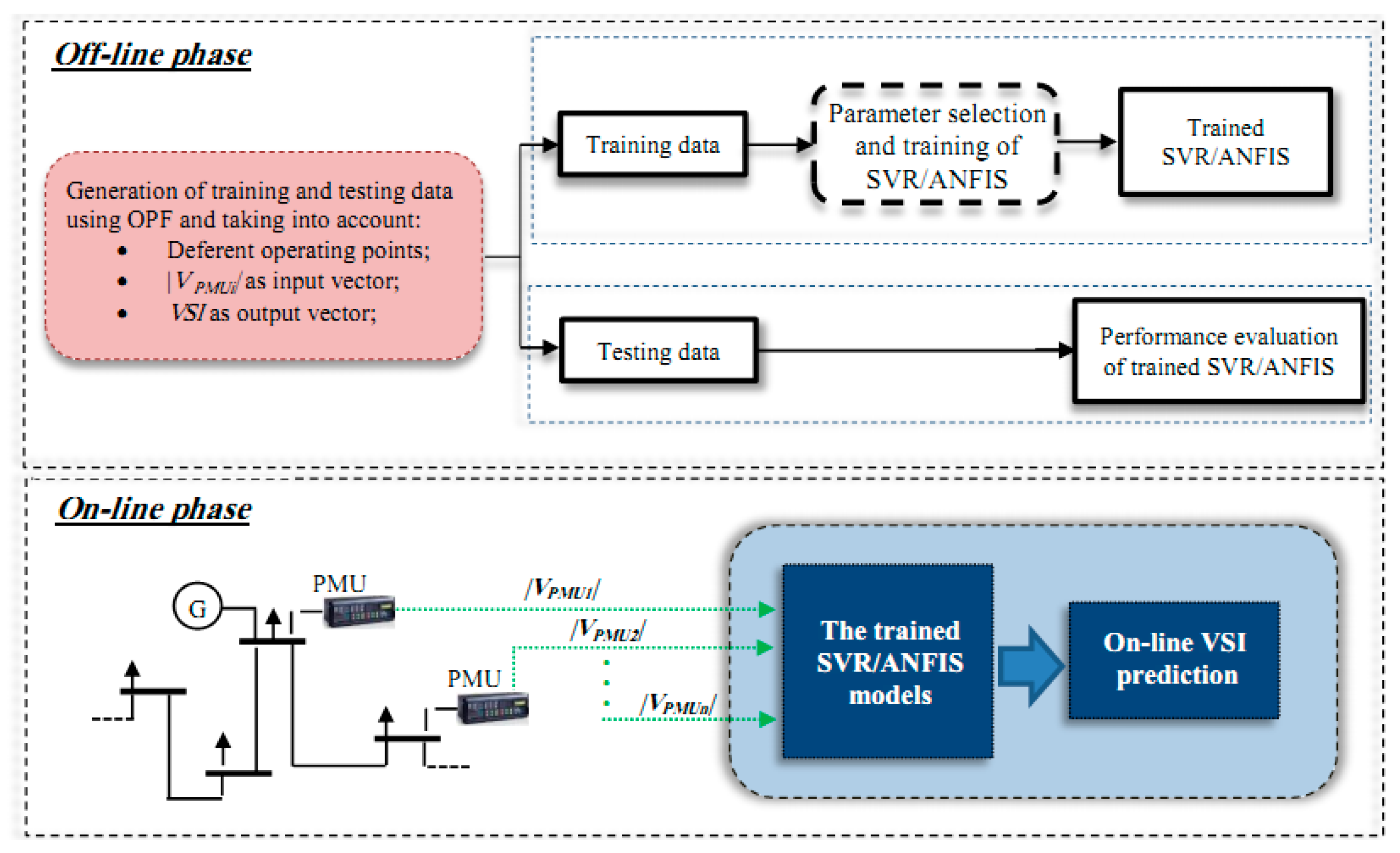
The proposed methodology deployed for an on-line assessment of voltage stability using the ALO-SVR and ANFIS models based PMUs measurements is illustrated in Figure 1. The proposed methodology incipient with an off-line training for the ALO-SVR and ANFIS models and the outcomes will be an on-line monitoring of voltage stability condition incurred in a power system. During the off-line phase of working procedure, the inputs and outputs are generated based on a conventional power flow required for the training and testing processes of ALO-SVR and ANFIS models until it culminates to a stage wherein the well trained and tested model is then conveyed for an on-line phase of working procedure. In the on-line phase of working procedure, the real-time information, or data obtained from the PMU devices are applied immediately to the well trained and tested SVR and ANFIS models to estimate the VSI required for the real-time risk assessment of power system.
4.1. Data Preparation for the Training and Testing
The first step perpetrated in the off-line process involves the data preparation for the training and testing procedure of the ALO-SVR and ANFIS. The training and testing data sets are generated by varying both of the real and reactive powers. The load is increased from the base case until the system reached the maximum loading point yielding to the collapse in a power system operation delineated by a non-executable power flow solution. Simultaneously, the VSI is calculated corresponding to the different operating points. In order to accommodate the increased power demand, the active power generation should be increased reciprocally. The increase in the generation can be carried out by the use of distributed slack bus method [49], or by the use of the optimal power flow (OPF) method. In this paper, the OPF technique [50] has been used. During its operation, the power systems face with a wide range of contingencies such as the loss of a transmission line, transformer or generating unit. When a contingency occurred, the power system configuration changes and leads to an inaccurate estimate of VSI by the trained models. In the present paper, a single line outage, which is the most frequent contingency that can appear, is considered. For a large power system, it is impractical and unnecessary to train the models for all of the possible contingencies; therefore, contingencies should be ranked according to their severity on voltage stability to identify the most critical situations.
The voltage magnitudes extracted from the buses where PMUs are installed are taken as the input variables of ALO-SVR and ANFIS models. In turn, the minimum corresponding values of VSI are considered as the output variables.
4.2. SVR Parameters Optimization
In order to obtain an effective SVR model with a good predictive ability, there are three parameters that necessitate being chosen carefully. These parameters include the penalty parameter C, the non-sensitivity coefficient ε and the kernel parameters (bandwidth of the Gaussian RBF kernel γ in this study). These parameters have a great importance in the regression accuracy and generalization performance of the SVR model [51]. In this paper, the recently developed ALO has been deployed to optimize the SVR parameters.
4.2.1. Antlion Optimizer (ALO)
Antlion optimizer (ALO) is a recently established new and efficient swarm intelligence optimization technique proposed by Mirjalili in 2015 [52]. It was inspired from the intelligent demeanor of antlion hunting mechanism for ants in nature. The mathematical modeling of ALO algorithm can be summarized in the follows procedures [52].
- Random movement of ants: In nature, the ants walk in a random way when seeking for food. This stochastic movement is given by Equation (23).where cumsum is the cumulative sum, t represents the step of a stochastic walk (iteration), and r(t) is a random function expressed by the following Equation.To confine the random walks within the search space, the ant movement must be normalized at every iteration as fellows.where Xit is the normalized value of the ith variable, t represents the iteration, ai and bi are respectively the min-max of the stochastic walk of the ith variable, cit and dit are the min-max of the stochastic walk of the ith variable at tth iteration, respectively.
- Trapping in antlion’s pits: The ant’s stochastic move is influenced by ant-lions’ traps, which can be modeled as follows.where ct and dt are the min-max of variables at tth iteration, respectively, Antliontjt indicates the position of the jth antlion at the tth iteration.
- Building trap and sliding ants toward ant lion: The ant-lions’ hunting capability can be modeled using the roulette wheel. The slipping of ants into ant lions pits is given by the Equation (27).where I is a ratio given as follows:where t and T are the current iteration and the total number of iterations, respectively.
- Catching ants and rebuilding the pit: when ant reaches the lowest part of the pit, the ant lion consumes it. To increase the opportunities for catching another ant, the ant lion takes the position of the latest caught prey and rebuild a novel pit. This process can be modeled as follows.where Antit is the position of ith ant at tth iteration.
- Elitism: The elite ant lion, which is the best ant lion obtained at every iteration, is saved and it must be competent to influence the locomotion of all the ants. Thus, it presumed that each ant unsystematically walks around a chosen ant lion by the roulette wheel and the elite at the same instant as follows:where RAt and REt are respectively the stochastic walks around the antlion chosen by the roulette wheel and round the elite at tth iteration.
4.2.2. Application of ALO in SVR Parameters Optimization
In this section, the ALO algorithm has been deployed to optimize the SVR parameters i.e., C, γ and ε. The proposed methodology can be briefly described by the following steps.
- Step 1:
- Set the initial parameters of ALO, which are: the number of ants and antlions, the maximum number of iterations, the number of variables (SVR parameters), and the upper/lower bounds of variables.
- Step 2:
- Initialize randomly the first population of ants and antlions.
- Step 3:
- Train the SVR model using the training set and compute the fitness value of ant and antlions. The root mean squared error (RMSE) was used as a fitness function.
- Step 4:
- Find the better ant lion and consider it as the elite.
- Step 5:
- For every antlion:
- Choose an antlion based on the roulette wheel
- Update the values of c and d utilizing Equation (27).
- Generate a stochastic move and normalize it using Equations (23) and (25).
- Update the location of ant based on Equation (30).
- Step 6:
- Compute the fitness of every ant.
- Step 7:
- Substitute an antlion with its corresponding ant if it is better using Equation (29).
- Step 8:
- Update the elite if an antlion becomes better.
- Step 9:
- Check the stopping criterion: if the stopping criterion is achieved go to the step 10. Otherwise, loop to the step 5.
- Step 10:
- The position of the elite comprised the optimum values of SVR parameters.
5. Results and Discussion
In order to investigate the performance of the proposed SVR and ANFIS models used as tools of prediction, the accuracy of predicted VSI will be analyzed for the case studies of IEEE 30-bus and IEEE 118-bus test systems. The important parameter values of these systems are given in Table 1 and the other detailed parameters can be retrieved from [53].
In the on-line assessment of voltage stability, the optimal number, and placement of phasor measurement technology based PMUs should be implemented beforehand in such a way that pervasive as well as a coherent observation on the network performance could be rendered with a minimum cost of investment and implementation. In order to obtain the optimal number and locations of PMUs with the aim of static state estimation, the systems were simulated in Power System Analysis Toolbox (PSAT) software version 2.1.5 [53]. The optimal number and locations of PMUs for both test systems are shown in Table 2. On the other hand, to identify the most critical contingencies, contingency analysis was carried out for all single line outages in both systems. The selected contingencies, for both test systems, along with their corresponding VSI in the base loading condition, are shown in Table 3.
The acquired outcomes i.e., the voltage magnitudes and phase angles measured from the PMUs will be used as the input information for the SVR and ANFIS models to estimate the on-line VSI.
5.1. Implementation of ALO-SVR and ANFIS Models in VSI Prediction
This sub-section will divulge on the performance of ALO-SVR and ANFIS models that are used to estimate the VSI of an IEEE 30-bus and IEEE 118-bus test systems. The models were trained and tested using the voltage magnitudes that were taken as the input variables procured from the PMUs right after the load flow solution is performed and the output variable for the models will be the prediction of minimum VSI. The training and testing data sets for both models are generated for the different loading conditions and critical contingencies. The subsequent step involved in the training and testing of ALO-SVR and ANFIS models is to identify the best structure and characteristics that will improve the performance of both models in prediction.
With respect to the development of optimal SVR structure, there are two main steps involved via the selection of kernel function and optimization of the values of penalty (C), ε and kernel parameters. In this research, the Gaussian RBF is used as the kernel function. The performance of the SVR based Gaussian RBF kernel is highly dependent on the RBF kernel width (γ). Unfortunately, there are no defined rules for determining the optimum values of C, ε, and γ since these values should be determined in accordance with the current situation of implementation. As aforementioned, the ALO algorithm seeks for the optimal values of C, γ, and ε parameters.
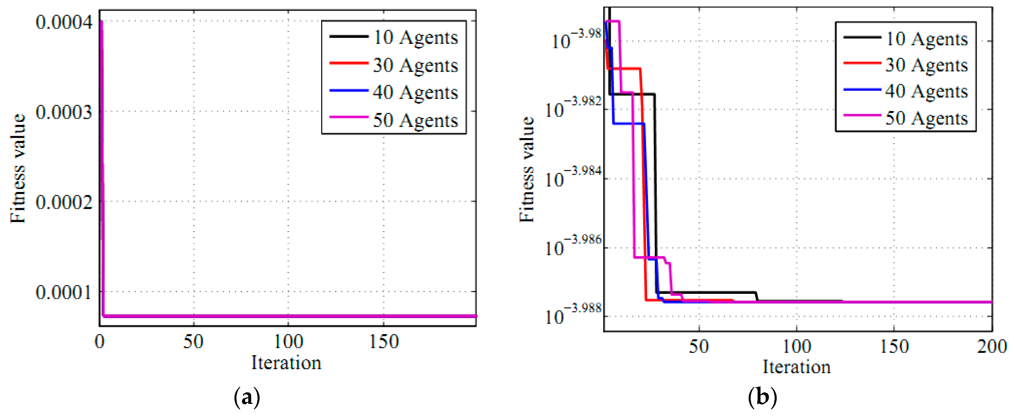
When using the ALO algorithm for identifying the optimal SVR parameters, some parameters must be determined, such as the maximum number of iterations, the number of search agents (candidate solutions), the fitness function, the number of variables, and the upper/lower bounds of variables. In the present study, the number of iterations was set to 200 with a various number of search agents (10, 30, 40, and 50) to evaluate the impact of these parameters on SVR performance. The RMSE was considered as a fitness function in the optimization process. Moreover, the stopping criterion in this study is the set number of maximum iteration. The ranges of C, γ, and ε parameters are as follows: [1 1000], [0.0001 0.1], and [0.1 1], respectively. The iterative RMSE trend of the ALO searching of the SVR optimal parameters in the training stage is displayed in Figure 2a,b. It can be seen from this figure that the ALO algorithms based 10, 30, 40, and 50 search agents can all achieve the best fitness values, which are 3.2718 × 10⁻⁴ and 1.0290 × 10⁻⁴ in the cases of IEEE 30-bus and IEEE 118-bus, respectively. However, there is a small difference among them in the convergence speed. The optimal found values of C, γ and ε parameters for both systems are shown in Table 4.
The subsequent implementation of SVR will be the subtractive clustering method that used to construct the ANFIS model for predicting the VSI. In order to generate fuzzy rules by using the subtractive clustering method, it is essential to determine a proper cluster radius (radii). According to [54], the recommended values for ‘radii’ should be in the range between 0.2 and 0.5. The RMSE results for different values of cluster radius in testing process are presented in Table 5. Based on the obtained results, a cluster radius of 0.2 and 0.4 are selected for the case studies of IEEE 30-bus system and IEEE 118-bus system, respectively, for the reason that these values are corresponding to the minimum RMSE.
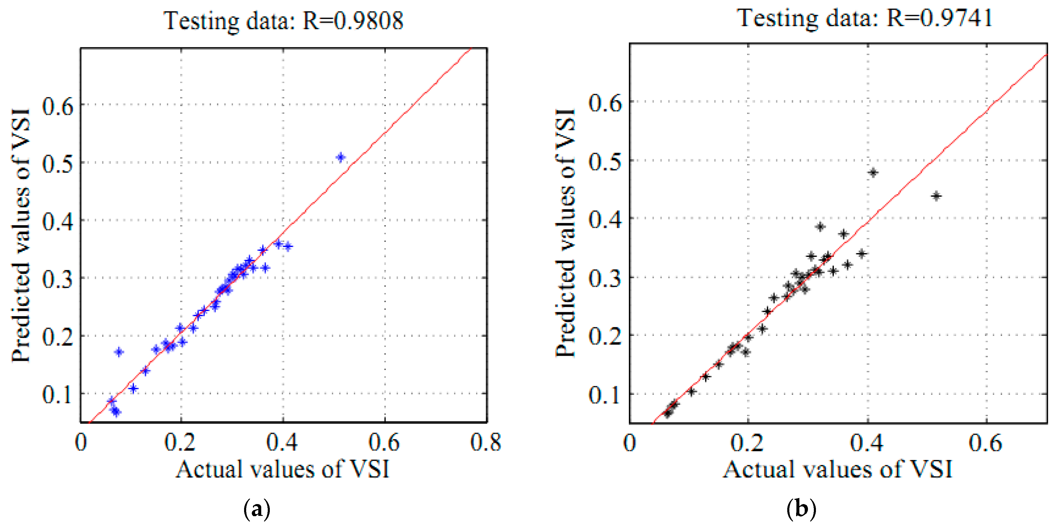
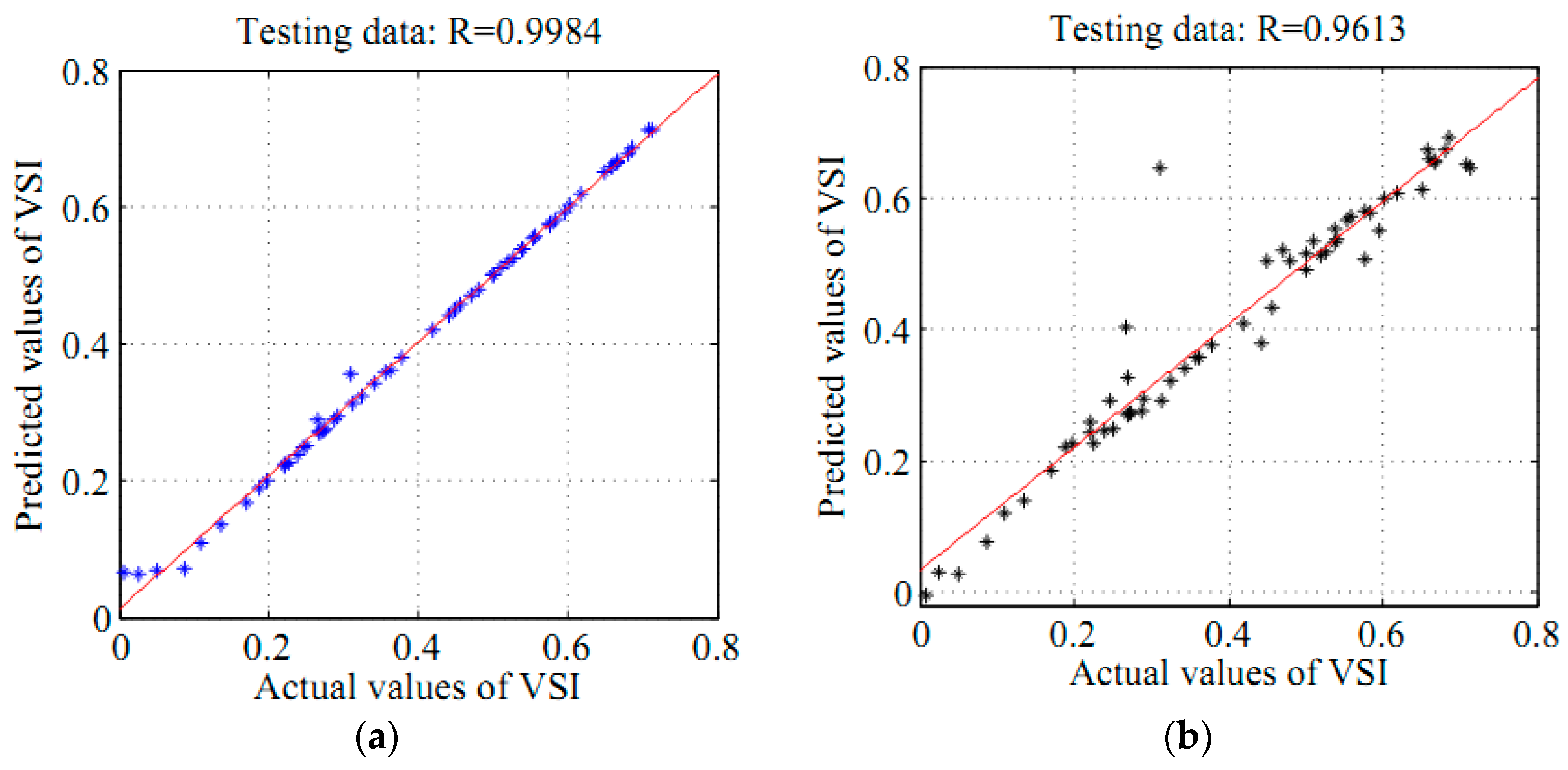
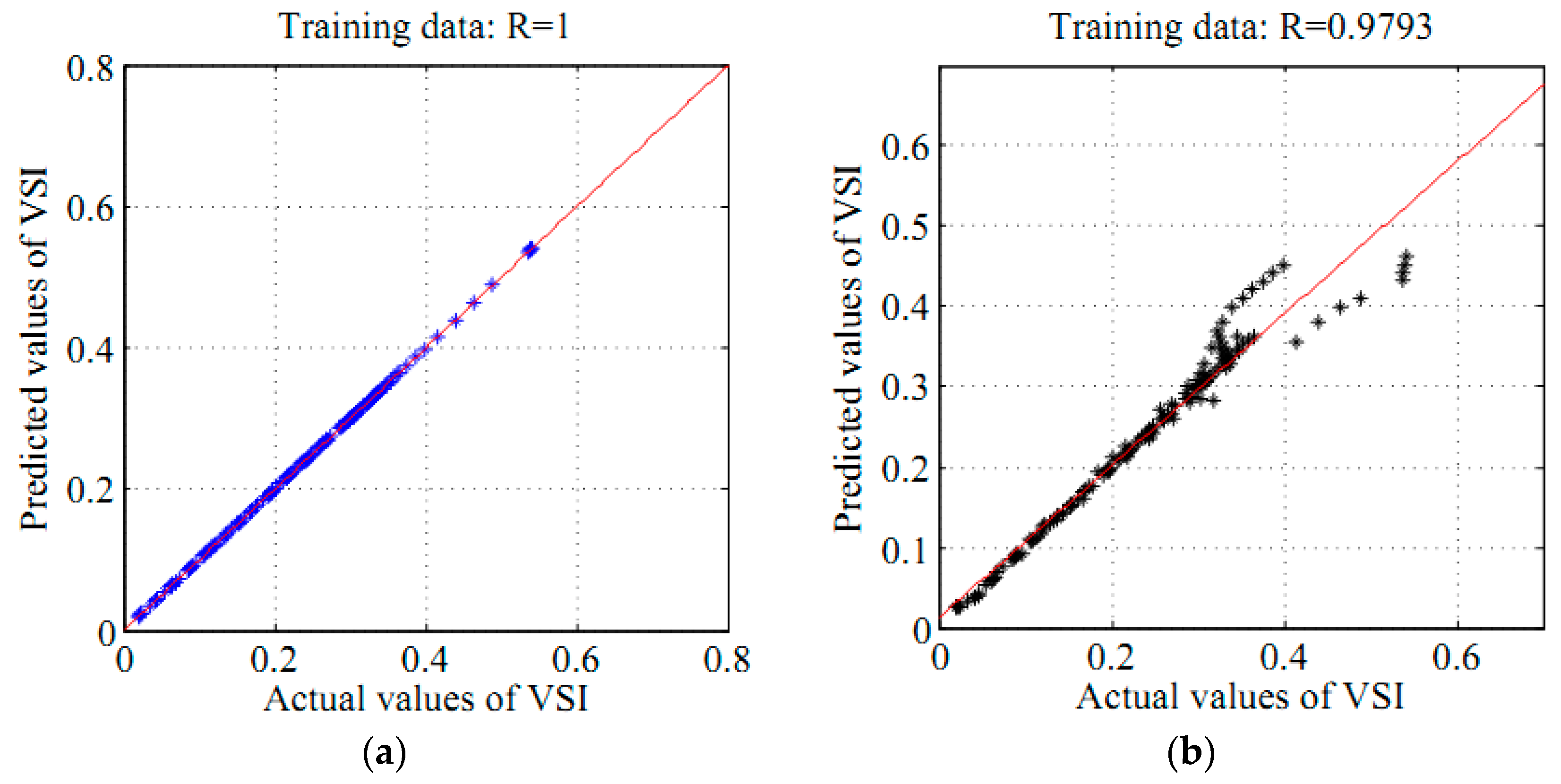
Once the optimal parameters of SVR and ANFIS models are obtained, the ability of both models in prediction of voltage stability margin was evaluated. In Figure 3 and Figure 4, the conventional load flow solution inflicting to the actual values of VSI is compared with the predicted values of VSI determined by using the training and testing processes of ANFIS and ALO-SVR models. Figure 3a,b, evince that the ALO-SVR provide the results that are in good agreement with the actual values in contrast with the ANFIS and this is referring to the case study of IEEE 30-bus system. The abovementioned discussion is similar with compendium, representing the outcome of ALO-SVR model for the cases study of IEEE 118-bus system as shown in Figure 4a,b. The linear fits between the actual and results predicted by the ANFIS and ALO-SVR models for the case of IEEE 30-bus system are illustrated in Figure 5 and Figure 6. It is obvious that the ALO-SVR model has a good prediction performance in both training and testing processes giving to the linear fits with the correlation coefficient (R) close to 1 when compared to the ANFIS model. This finding is supported by comparing the correlation coefficients (R) of 1 and 0.9947 obtained from the ALO-SVR and ANFIS training processes, respectively. Withal the findings are also supported based on the comparison between the correlation coefficients (R) of 0.9984 and 0.9613 determined corresponding to the output of SVR and ANFIS testing processes, respectively. Hence, the comparison revealed that the ALO-SVR performs a better prediction than the ANFIS either during the training or testing processes. Robustness of the SVR used to predict the VSI compared to the ANFIS for the IEEE 118-bus system is also shown in Figure 7 and Figure 8. The finding is proven particularly referring to the R of 1 and 0.9793 for the ALO-SVR and ANFIS training processes, respectively. Similarly, the ensuing particular also corroborates the findings such that the R of 0.9807 and 0.9741 for the ALO-SVR and ANFIS testing processes, respectively. These values show that the ALO-SVR prediction is better than the ANFIS prediction.
In order to further assess the performance of ALO-SVR model to discern with the ANFIS model, the performance indicator predicated by the root mean square error will be used in the comparative analysis. The model’s performance towards training and testing processes for the case studies of IEEE 30-bus and IEEE 118-bus systems is expounded in Table 6. The statistical error obtained from training process indicated that the ALO-SVR model produced relatively lower RMSE of 3.2718 × 10⁻⁴ for the case study of IEEE 30-bus and 1.0290 × 10⁻⁴ for the case study of IEEE 118-bus than the results provided using the ANFIS model which is 0.0209 for the case of IEEE 30-bus and 0.0238 for the case of IEEE 118-bus. For the testing process, the RMSE values of 0.0118 and 0.0535 are obtained by the ALO-SVR and ANFIS models for the case study of IEEE 30-bus system, respectively. For the case study of IEEE 118-bus system, the predictions are resulting to the RMSE of 0.0230 for ALO-SVR testing process and RMSE of 0.0238 for ANFIS testing process. From the obtained results, it is clear that the ALO-SVR model acquired relatively smaller RMSE and larger R contradictory with the ANFIS model during both training and testing processes. In other words, the ALO-SVR performance culminates in giving the best prediction results than the ANFIS model. Table 6 shows the results of the comparative study between the ALO-SVR and ANFIS models for both test systems.
5.2. Impact of PMUs Outage on ALO-SVR Performance
The effectiveness of the proposed ALO-SVR model in the estimation of VSI was also checked in the case of PMUs loss contingency. Table 7 lists the performance indices of three test scenarios with PMUs outage for both test systems. These scenarios include the outages of one, two, and three PMUs in both case studies of IEEE 30-bus and IEEE 118-bus test systems. From the Table 7, it can be seen that the proposed ALO-SVR model is still able to accurately predict the VSI when PMUs outage is considered.
6. Conclusions
In this paper, the use of SVR and ANFIS based synchrophasor measurements for on-line voltage stability assessment has been presented. The antlion optimizer (ALO) algorithm is adopted as a search strategy to seek for the optimal parameters of SVR and a new hybrid model, namely ALO-SVR, model is proposed. The voltage magnitudes obtained from PMUs, for both the base case and for a selected number of contingencies, are used as the input variables of ALO-SVR and ANFIS models, while the output variables are the minimum values of VSI. The performances of the two models are evaluated in terms of the correlation coefficient (R) and RMSE. The results suggested that the two models can be successfully applied to predict the VSI. However, the ALO-SVR model gave a better performance than the ANFIS model. The study showed also the impact of PMUs loss contingency on the predictive ability of the ALO-SVR. The results revealed that the model is able to accurately predict the VSI in the case of PMUs loss contingency.
Acknowledgments
The authors would like to acknowledge The Institute of Research Management and Innovation (IRMI) UiTM, Shah Alam, Selangor, Malaysia for the financial support of this research. This research is supported by IRMI under the BESTARI Research Grant Scheme with project code: 600-IRMI/MYRA 5/3/BESTARI (027/2017).
Author Contributions
Mohammed Amroune contributed in designing and developing the proposed methodology and implemented the Matlab code. Ismail Musirin, Tarek Bouktir and Muhammad Murtadha Othman contributed in analyzing and interpret the simulation results. The main revisions were done by all of the authors before finalizing the manuscript.
Conflicts of Interest
The authors declare no conflict of interest.
References
- Kanimozhi, R.; Selvi, K.; Balaji, S. Multi-objective approach for load shedding based on voltage stability index consideration. Alex. Eng. J. 2014, 53, 817–825. [Google Scholar] [CrossRef]
- Dan, S.; Sidhu, T.S. Application of compressive sampling in synchrophasor data communication in WAMS. IEEE Trans. Ind. Inform. 2014, 10, 450–460. [Google Scholar]
- Maria, L.; Michael, L. A review of the development of smart grid technologies. Renew. Sustain. Energy Rev. 2016, 59, 710–725. [Google Scholar]
- Nazari-Heris, M.; Mohammadi-Ivatloo, B. Application of heuristic algorithms to optimal PMU placement in electric power systems: An updated review. Renew. Sustain. Energy Rev. 2015, 50, 214–228. [Google Scholar] [CrossRef]
- Mousavi, O.; Cherkaoui, R. Investigation of P–V and V–Q based optimization methods for voltage and reactive power analysis. Electr. Power Energy Syst. 2014, 63, 769–778. [Google Scholar] [CrossRef]
- Milano, F. Continuation power flow analysis. In Power System Modeling and Scripting; Springer: Berlin/Heidelberg, Germany, 2015; pp. 103–130. [Google Scholar]
- Modarresi, J.; Gholipour, E.; Khodabakhshian, A. A comprehensive review of the voltage stability indices. Renew. Sustain. Energy Rev. 2016, 63, 1–12. [Google Scholar] [CrossRef]
- Debbie, Q.; Zhou, U.; Annakkage, D. Online Monitoring of Voltage Stability Margin Using an Artificial Neural Network. IEEE Trans. Power Syst. 2010, 25, 1566–1574. [Google Scholar]
- Chakrabarti, S. Voltage stability monitoring by artificial neural network using a regression-based feature selection method. Expert Syst. Appl. 2008, 35, 1802–1808. [Google Scholar] [CrossRef]
- Jayasankar, V.; Kamaraj, N.; Vanaja, N. Estimation of voltage stability index for power system employing artificial neural network technique and TCSC placement. Neurocomputing 2010, 73, 3005–3011. [Google Scholar] [CrossRef]
- Syed, A.; Ankur, G.; Dinesh, K.; Saikat, C. Voltage stability monitoring of power systems using reduced network and artificial neural network. Electr. Power Energy Syst. 2017, 87, 43–51. [Google Scholar]
- Chakrabarti, S.; Jeyasurya, B. An enhanced Radial Basis Function Network for voltage stability monitoring considering multiple contingencies. Electr. Power Syst. Res. 2007, 77, 780–787. [Google Scholar] [CrossRef]
- Chakrabarti, S.; Jeyasurya, B. Multi-contingency voltage stability monitoring of a power system using an adaptive radial basis function network. Electr. Power Energy Syst. 2008, 30, 1–7. [Google Scholar] [CrossRef]
- Devaraj, D.; Preetha, J. On-line voltage stability assessment using radial basis function network model with reduced input features. Electr. Power Energy Syst. 2011, 33, 1550–1555. [Google Scholar] [CrossRef]
- Javan, D.; Mashhadi, H.; Rouhani, M. A fast static security assessment method based on radial basis function neural networks using enhanced clustering. Electr. Power Energy Syst. 2013, 44, 988–996. [Google Scholar] [CrossRef]
- Hashemi, S.; Aghamohammadi, M. Wavelet based feature extraction of voltage profile for online voltage stability assessment using RBF neural network. Electr. Power Energy Syst. 2013, 49, 86–94. [Google Scholar] [CrossRef]
- Handschin, E.; Kuhlmann, D.; Rehtazn, C. Visualisation and analysis of voltage stability using Self-Organizing neural network. In Artificial Neural Network—ICANN’97; Lecture Notes in Computer Science, 1327; Springer: Berlin/Heidelberg, Germany, 1997. [Google Scholar]
- Chakraborty, K.; De, A.; Chakrabarti, A. Voltage stability assessment in power network using self-organizing feature map and radial basis function. Comput. Electr. Eng. 2012, 38, 819–826. [Google Scholar] [CrossRef]
- Duraipandy, P.; Devaraj, D. Extreme Learning Machine Approach for On-Line Voltage Stability Assessment. Swarm Evolut. Emotic Comput. 2013, 8298, 397–405. [Google Scholar]
- Berizzi, A.; Bovo, C.; Delfanti, M.; Merlo, M.; Pozzi, M. A Neuro-Fuzzy Inference System for the Evaluation of Voltage Collapse Risk Indices. In Proceedings of the Bulk Power System Dynamics and Control—VI, Cortina d’Ampezzo, Italy, 22–27 August 2004. [Google Scholar]
- Zheng, C.; Malbasa, V.; Kezunovic, M. A Fast Stability Assessment Scheme based on Classification and Regression Tree. In Proceedings of the IEEE International Conference on Power System Technology, Auckland, New Zealand, 30 October–2 November 2012. [Google Scholar]
- Li, Z.; Wu, W. Phasor Measurements-Aided Decision Trees for Power System Security Assessment. In Proceedings of the Second International Conference on Information and Computing Science, Manchester, UK, 21–22 May 2009. [Google Scholar]
- Beiraghi, M.; Ranjbar, A. Online Voltage Security Assessment Based on Wide-Area Measurements. IEEE Trans. Power Deliv. 2013, 28, 989–997. [Google Scholar] [CrossRef]
- Bruno, L.; Venkataramana, A. Development of Multilinear Regression Models for Online Voltage Stability Margin Estimation. IEEE Trans. Power Syst. 2011, 26, 374–383. [Google Scholar]
- Torres, P.; Peralta, H.; Castro, A. Power System Loading Margin Estimation Using a Neuro-Fuzzy Approach. IEEE Trans. Power Syst. 2007, 22, 1955–1964. [Google Scholar] [CrossRef]
- Modi, P.; Singh, S.; Sharma, J. Fuzzy neural network based voltage stability evaluation of power systems with SVC. Appl. Soft Comput. 2008, 8, 657–665. [Google Scholar] [CrossRef]
- Vapnik, V. The Nature of Statistical Learning Theory; Springer: New York, NY, USA, 1995. [Google Scholar]
- Suganyadevi, M.V.; Babulal, C.K. Support Vector Regression Model for the prediction of Loadability Margin of a Power System. Appl. Soft Comput. 2014, 24, 304–315. [Google Scholar] [CrossRef]
- Cortés-Carmona, M.; Jiménez-Estévez, G.; Guevara-Cedeño, J. Support Vector Machines for On-Line Security Analysis of Power Systems. In Proceedings of the Transmission and Distribution Conference and Exposition: Latin America, 2008 IEEE/PES, Bogota, Colombia, 13–15 August 2008. [Google Scholar]
- Mohammadi, M.; Gharehpetian, G. Power System on-line Static Security Assessment by using Multi-Class Support Vector Machines. J. Appl. Sci. 2008, 8, 2226–2233. [Google Scholar] [CrossRef]
- Kalyani, S.; Swarup, K. Classification of Static Security Status Using Multi-Class Support Vector Machines. TJER 2012, 9, 21–30. [Google Scholar] [CrossRef]
- Suganyadevi, M.; Babulal, C. Fast Assessment of Voltage Stability Margin of a Power System. J. Electr. Syst. 2014, 10, 305–316. [Google Scholar]
- Schölkopf, B.; Smola, J. Learning with Kernels. Ph.D. Thesis, Technische Universität Berlin, Birlinghoven, Germany, 1998. [Google Scholar]
- Utpal, K.; Kok, S.; Mehdi, S.; Mohd, Y.; Saad, M.; Ben, H.; Alex, S. SVR-Based Model to Forecast PV Power Generation under Different Weather Conditions. Energies 2017, 10, 876. [Google Scholar]
- Hsu, C.; Chang, C.; Lin, C. A Practical Guide to Support Vector Classification. Available online: www.datascienceassn.org/sites/default/files/Practical%20Guide%20to%20Support%20Vector%20Classification.pdf (accessed on 19 October 2017).
- Chung, K.; Kao, W.; Sun, C.; Wang, L.; Lin, C. Radius margin bounds for support vector machines with the RBF kernel. Neural Comput. 2003, 15, 2643–2681. [Google Scholar] [CrossRef] [PubMed]
- Al-Shammari, E.; Keivani, A.; Shamshirband, S.; Mostafaeipour, A.; Yee, P.; Petkovi, L.; Sudheer, C. Prediction of heat load in district heating systems by Support Vector Machine with Firefly searching algorithm. Energy 2016, 95, 266–273. [Google Scholar] [CrossRef]
- Sajan, K.S.; Vishal, K.; Barjeev, T. Genetic algorithm based support vector machine for on-line voltage stability monitoring. Electr. Power Energy Syst. 2015, 73, 200–208. [Google Scholar] [CrossRef]
- Hu, W.; Kaizeng, Y.; Wang, H. A Short-term Traffic Flow Forecasting Method Based on the Hybrid PSO-SVR. Neural Process. Lett. 2016, 43, 155–172. [Google Scholar] [CrossRef]
- García Nieto, P.; García-Gonzalo, E.; Alonso Fernández, J.; Díaz Muñiz, C. A hybrid wavelet kernel SVM-based method using artificial bee colony algorithm for predicting the cyan toxin content from experimental cyanobacteria concentrations in the Trasona reservoir (Northern Spain). J. Comput. Appl. Math. 2017, 309, 587–602. [Google Scholar] [CrossRef]
- Aldeen, M.; Sahaa, S.; Alpcana, T.; Evans, R. New online voltage stability margins and risk assessment for multi-bus smart power grids. Int. J. Control 2015, 88, 1–15. [Google Scholar] [CrossRef]
- Alpcana, M.; Sahaa, T.; Aldeen, S. Assessment of voltage stability risks under intermittent renewable generation. In Proceedings of the IEEE PES General Meeting|Conference & Exposition, National Harbor, MD, USA, 27–31 July 2014. [Google Scholar]
- Ismail, M.; Khawa, A. Novel Fast Voltage Stability Index (FVSI) for Voltage Stability Analysis in Power Transmission System. In Proceedings of the Student Conference on Research and Development, Shah Alam, Malaysia, 16–17 July 2002. [Google Scholar]
- Salehi, V.; Mohammed, O. Real-Time Voltage Stability Monitoring and Evaluation Using Synchorophasors. In Proceedings of the IEEE North American Power Symposium, Boston, MA, USA, 4–6 August 2011. [Google Scholar]
- Drucker, H.; Burges, C.; Kaufman, L.; Smola, A.; Vapnik, V. Support Vector Regression Machines. In Proceedings of the 1996 Conference on Advances in Neural Information Processing Systems; MIT Press: Cambridge, MA, USA, 1997; pp. 155–161. [Google Scholar]
- Jang, J.-S.R. ANFIS: Adaptive-network-based fuzzy inference system. IEEE Trans. Power Syst. Man Cybern. Syst. 1993, 23, 665–685. [Google Scholar] [CrossRef]
- Chiu, S. Fuzzy model identification based on cluster estimation. J. Intell. Fuzzy Syst. 1994, 2, 267–278. [Google Scholar]
- Chiu, S. Method and software for extracting fuzzy classification rules by subtractive clustering. In Proceedings of the Fuzzy Information Processing Society, NAFIPS Biennial Conference of the North American, Berkeley, CA, USA, 19–22 June 1996. [Google Scholar]
- Tong, S.; Miu, K. A Participation Factor Model for Slack Buses in Distribution Systems with DGs. In Proceedings of the 2003 IEEE/PES Transmission & Distribution Conference, Dallas, TX, USA, 7–12 September 2003. [Google Scholar]
- Amroune, M.; Bourzami, A.; Bouktir, T. Weakest buses identification and ranking in large power transmission network by optimal location of reactive power support. TELKOMNIKA Indones. J. Electr. Eng. 2014, 12, 7123–7130. [Google Scholar] [CrossRef]
- Li, X.L.; Li, L.H.; Zhang, B.L.; Guo, Q.J. Hybrid self-adaptive learning based particle swarm optimization and support vector regression model for grade estimation. Neurocomputing 2013, 118, 179–190. [Google Scholar] [CrossRef]
- Mirjalili, S. The ant lion optimizer. Adv. Eng. Softw. 2015, 83, 80–98. [Google Scholar] [CrossRef]
- Milano, F. Power System Analysis Toolbox (PSAT). Available online: http://faraday1.ucd.ie/psat.html (accessed on 19 October 2017).
- Gopalakrishnan, K.; Ceylan, H.; Attoh-Okine, O. Intelligent and Soft Computing in Infrastructure Systems Engineering; Springer: Berlin/Heidelberg, Germany, 2009. [Google Scholar]
Figure 1.
Block diagram of the proposed on-line voltage stability assessment method.

Figure 2.
Convergence curve of antlion optimizer (ALO) algorithm for (a) IEEE 30-bus; (b) IEEE 118-bus.
Figure 2.
Convergence curve of antlion optimizer (ALO) algorithm for (a) IEEE 30-bus; (b) IEEE 118-bus.

Figure 3.
Comparisons between the actual and predicted values of VSI of IEEE 30-bus in (a) Training process; (b) Testing process.
Figure 3.
Comparisons between the actual and predicted values of VSI of IEEE 30-bus in (a) Training process; (b) Testing process.
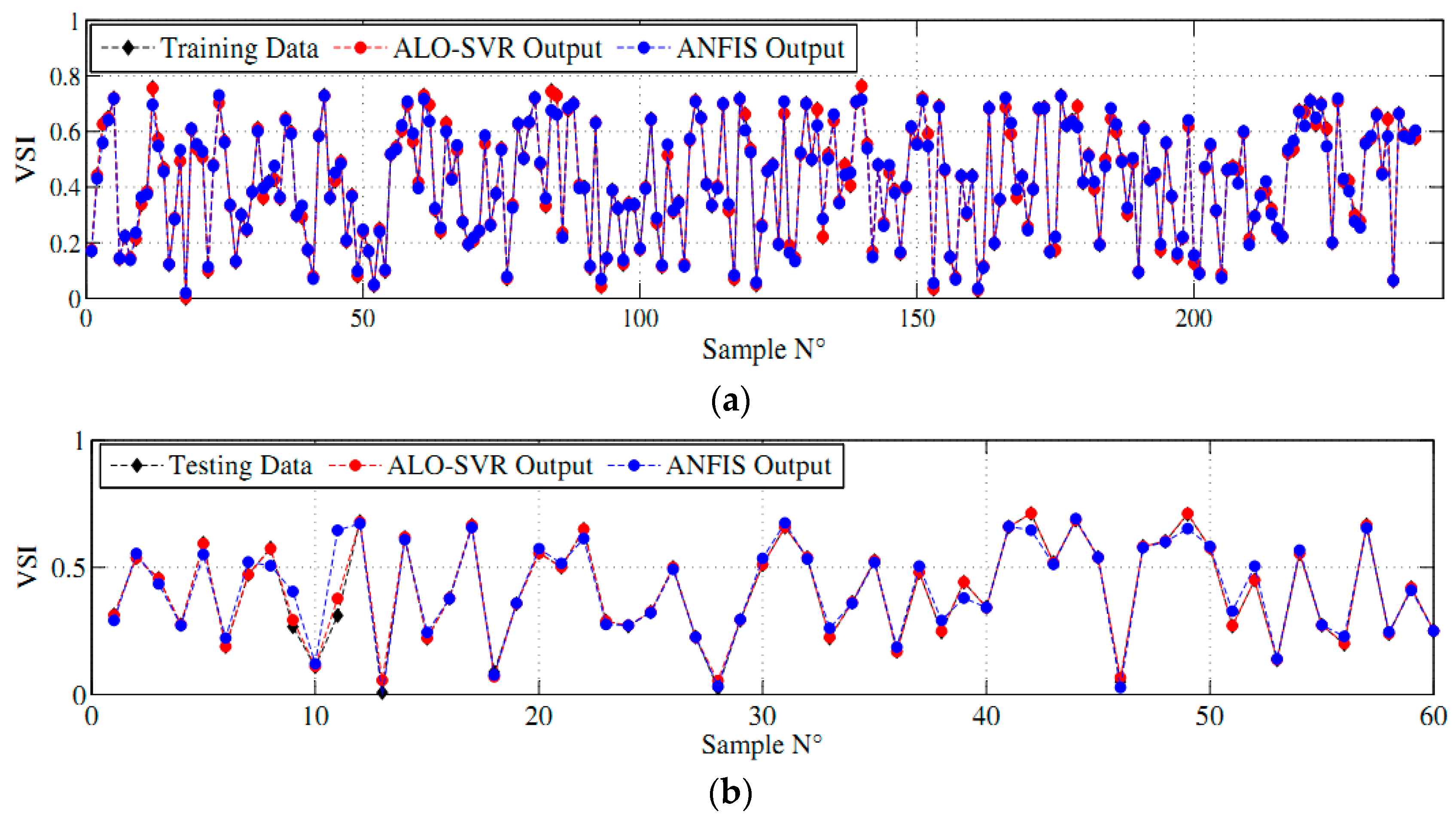
Figure 4.
Comparisons between the actual and predicted values of VSI for IEEE 118-bus in (a) Training process; (b) Testing process.
Figure 4.
Comparisons between the actual and predicted values of VSI for IEEE 118-bus in (a) Training process; (b) Testing process.
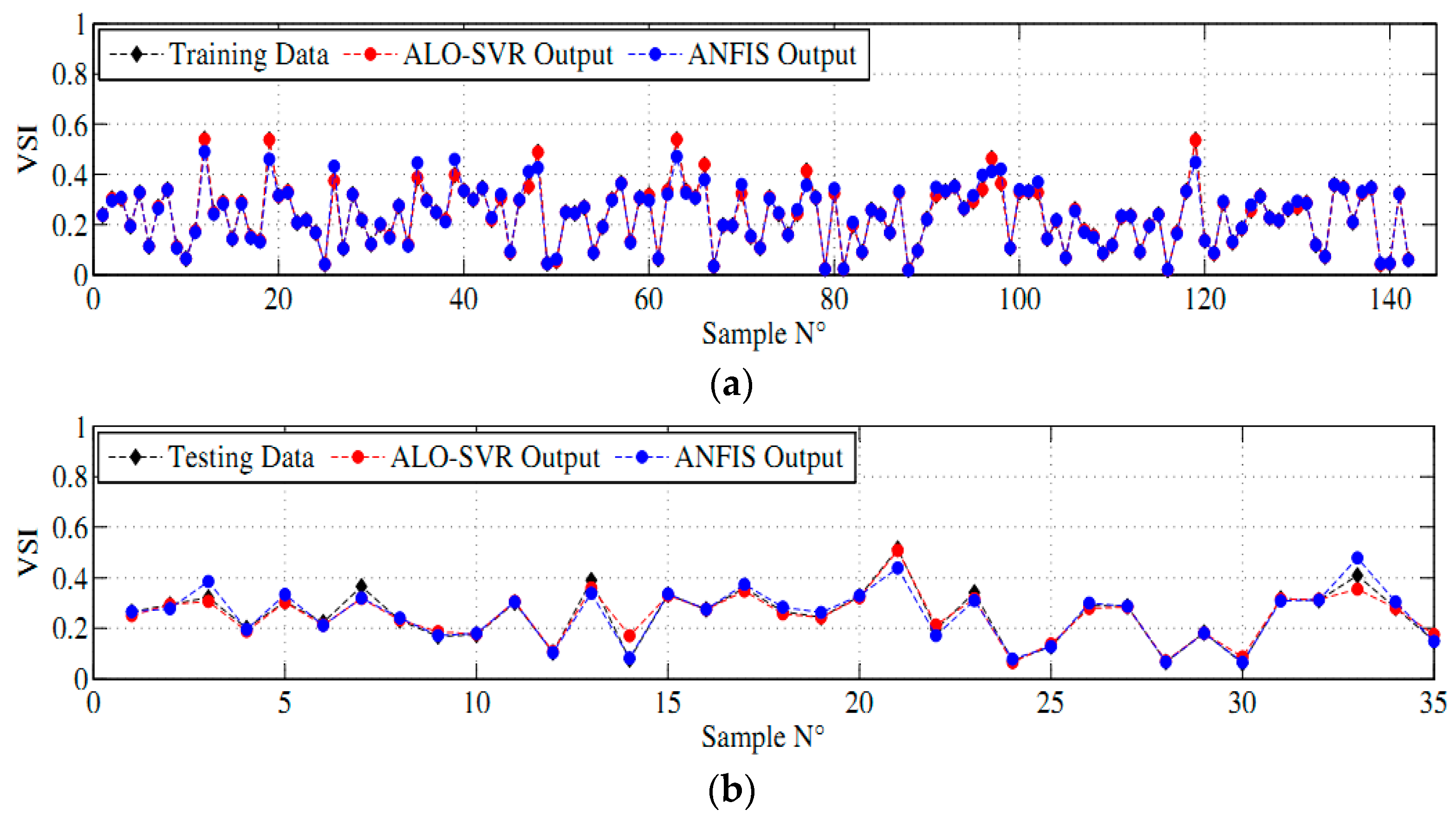
Figure 5.
Linear fits between the actual and predicted VSI for IEEE 30-bus in training phase using (a) ALO-SVR; (b) ANFIS.
Figure 5.
Linear fits between the actual and predicted VSI for IEEE 30-bus in training phase using (a) ALO-SVR; (b) ANFIS.
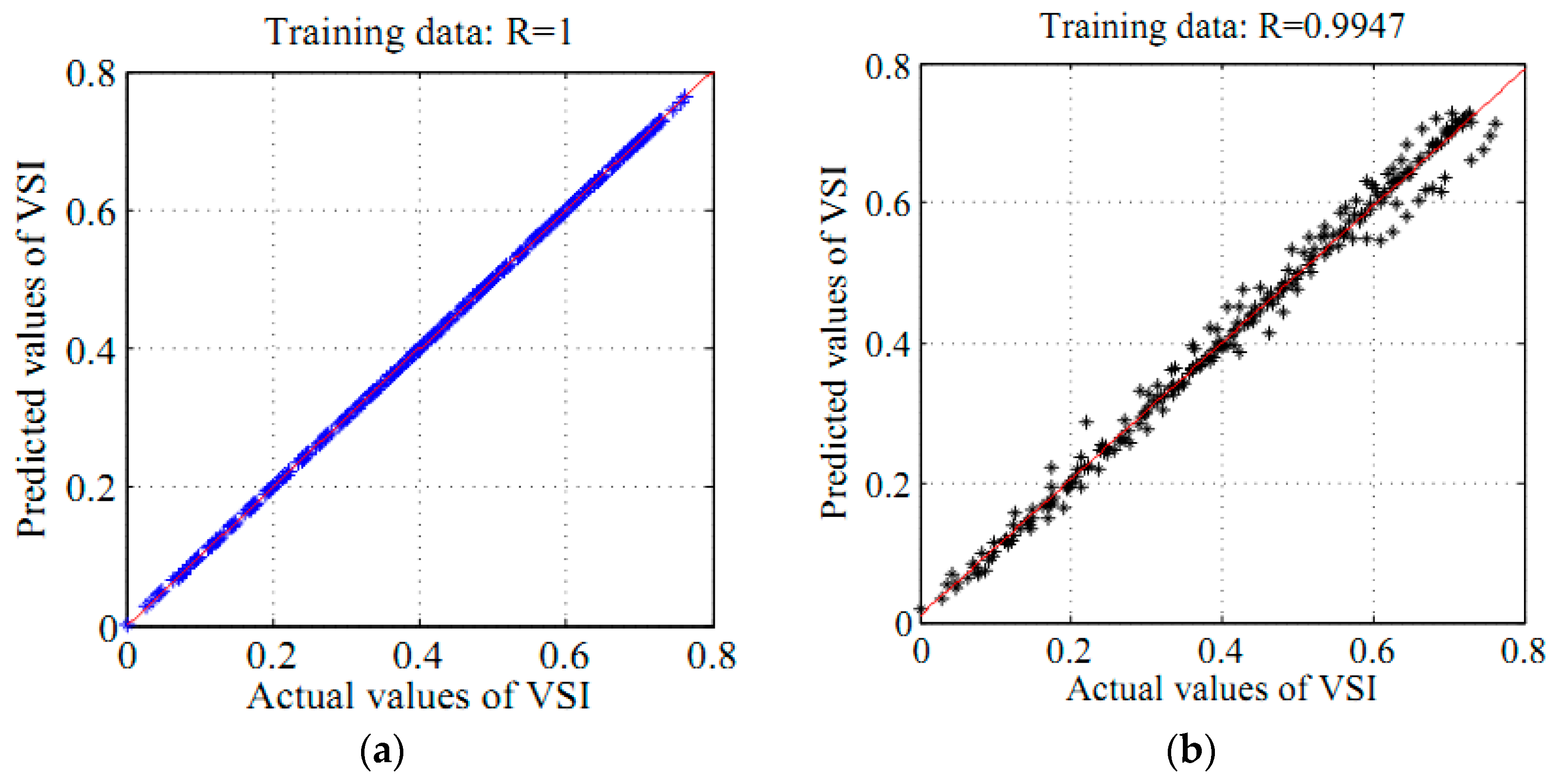
Figure 6.
Linear fits between the actual and predicted VSI for IEEE 30-bus in testing phase using (a) ALO-SVR; (b) ANFIS.
Figure 6.
Linear fits between the actual and predicted VSI for IEEE 30-bus in testing phase using (a) ALO-SVR; (b) ANFIS.

Figure 7.
Linear fits between the actual and predicted VSI for IEEE 118-bus in training phase using (a) ALO-SVR; (b) ANFIS.
Figure 7.
Linear fits between the actual and predicted VSI for IEEE 118-bus in training phase using (a) ALO-SVR; (b) ANFIS.

Figure 8.
Linear fits between the actual and predicted VSI for IEEE 118-bus in testing phase using (a) ALO-SVR; (b) ANFIS.
Figure 8.
Linear fits between the actual and predicted VSI for IEEE 118-bus in testing phase using (a) ALO-SVR; (b) ANFIS.

Table 1.
Important information of IEEE 30-bus and IEEE 118-bus test systems.
| Test System | Number of Generators | Number of Lines | Number of Loads | Total PL (MW) | Total QL (MVAr) | Number of OLTC |
|---|---|---|---|---|---|---|
| IEEE 30-bus | 6 | 41 | 24 | 283.4 | 126.2 | 4 |
| IEEE 118-bus | 54 | 186 | 64 | 3678 | 1438 | 9 |
Table 2.
Optimal number and location of phasor measurement units (PMUs) for the IEEE 30-bus and IEEE 118-bus test systems.
Table 2.
Optimal number and location of phasor measurement units (PMUs) for the IEEE 30-bus and IEEE 118-bus test systems.
| Test System | Number of Required PMUs | Location of PMUs |
|---|---|---|
| IEEE 30-bus | 7 | 3, 5, 10, 12, 19, 23, 27 |
| IEEE 118-bus | 31 | 2, 5, 9, 12, 13, 17, 21, 27, 29, 32, 34, 37, 40, 45, 49, 53, 56, 59, 66, 70, 71, 77, 80, 85, 86, 90, 94, 101, 105, 110, 118 |
Table 3.
Set of the critical contingencies for IEEE 30-bus and 118-bus test systems.
| Contingency No | IEEE 30-Bus System | IEEE 118-Bus System | ||
|---|---|---|---|---|
| Line Outage | VSI | Line Outage | VSI | |
| 1 | 1–2 | 0.3105 | 63–66 | 0.0146 |
| 2 | 6–7 | 0.5911 | 81–90 | 0.0148 |
| 3 | 2–5 | 0.7037 | 85–87 | 0.2690 |
| 4 | 9–10 | 0.7046 | 81–82 | 0.3082 |
| 5 | 4–6 | 0.7097 | 87–100 | 0.3094 |
| 6 | 5–7 | 0.7171 | 82–83 | 0.3219 |
| 7 | 2–6 | 0.7190 | 80–82 | 0.3474 |
| 8 | 1–3 | 0.7281 | 105–101 | 0.3597 |
| 9 | 4–12 | 0.7285 | 103–105 | 0.3649 |
| 10 | 12–13 | 0.7292 | 87–99 | 0.4096 |
| Intact condition | All lines are in service | 0.7622 | All lines are in service | 0.5406 |
Table 4.
Optimal parameters of SVR model found using ALO algorithm.
| SVR Parameters | Optimal Values of SVR Parameters | |
|---|---|---|
| IEEE 30-Bus | IEEE 118-Bus | |
| C | 679.673 | 569.824 |
| γ | 0.1 | 0.11169 |
| ε | 0.0001 | 0.0001 |
Table 5.
Selection of the best ‘Radii’ value of ANFIS model.
| Test System | Performance Index | ‘Radii’ Value | |||
|---|---|---|---|---|---|
| 0.2 | 0.3 | 0.4 | 0.5 | ||
| IEEE 30-bus | RMSE | 0.0210 | 0.0373 | 0.0749 | 0.0735 |
| IEEE 118-bus | RMSE | 0.0261 | 0.0244 | 0.0238 | 0.0292 |
Table 6.
Statistical coefficient of actual and predicted values.
| Test System | Parameters | ALO-SVR | ANFIS |
|---|---|---|---|
| IEEE 30-bus | Training RMSE | 3.2718 × 10⁻⁴ | 0.0209 |
| Training R | 1 | 0.9947 | |
| Testing RMSE | 0.0118 | 0.0535 | |
| Testing R | 0.9984 | 0.9613 | |
| IEEE 118-bus | Training RMSE | 01.0290 × 10⁻⁴ | 0.0238 |
| Training R | 1 | 0.9793 | |
| Testing RMSE | 0.0230 | 0.0238 | |
| Testing R | 0.9808 | 0.9741 |
Table 7.
ALO-SVR performance with PMUs outage.
| Test System | Number of PMUs | RMSE | R |
|---|---|---|---|
| IEEE 30-bus | 0 | 0.0118 | 0.9984 |
| 1 | 0.0168 | 0.9975 | |
| 2 | 0.0423 | 0.9815 | |
| 3 | 0.0584 | 0.9626 | |
| IEEE 118-bus | 0 | 0.0230 | 0.9808 |
| 1 | 0.0247 | 0.9808 | |
| 2 | 0.0251 | 0.9807 | |
| 3 | 0.0317 | 0.9806 |
© 2017 by the authors. Licensee MDPI, Basel, Switzerland. This article is an open access article distributed under the terms and conditions of the Creative Commons Attribution (CC BY) license (http://creativecommons.org/licenses/by/4.0/).
Share and Cite
MDPI and ACS Style
Amroune, M.; Musirin, I.; Bouktir, T.; Othman, M.M. The Amalgamation of SVR and ANFIS Models with Synchronized Phasor Measurements for On-Line Voltage Stability Assessment. Energies 2017, 10, 1693. https://doi.org/10.3390/en10111693
AMA Style
Amroune M, Musirin I, Bouktir T, Othman MM. The Amalgamation of SVR and ANFIS Models with Synchronized Phasor Measurements for On-Line Voltage Stability Assessment. Energies. 2017; 10(11):1693. https://doi.org/10.3390/en10111693
Chicago/Turabian StyleAmroune, Mohammed, Ismail Musirin, Tarek Bouktir, and Muhammad Murtadha Othman. 2017. "The Amalgamation of SVR and ANFIS Models with Synchronized Phasor Measurements for On-Line Voltage Stability Assessment" Energies 10, no. 11: 1693. https://doi.org/10.3390/en10111693
Note that from the first issue of 2016, this journal uses article numbers instead of page numbers. See further details here.