The Fuzzy Logic Method to Efficiently Optimize Electricity Consumption in Individual Housing


Research Group on Materials, Microelectronics, Acoustics, and Nanotechnology, University of Tours, 37000 Tours, France
*
Author to whom correspondence should be addressed.
Energies 2017, 10(11), 1701; https://doi.org/10.3390/en10111701
Submission received: 28 September 2017
/
Revised: 12 October 2017
/
Accepted: 24 October 2017
/
Published: 25 October 2017
(This article belongs to the Special Issue Decentralised Energy Supply Systems)
Abstract
:Electricity demand shifting and reduction still raise a huge interest for end-users at the household level, especially because of the ongoing design of a dynamic pricing approach. In particular, end-users must act as the starting point for decreasing their consumption during peak hours to prevent the need to extend the grid and thus save considerable costs. This article points out the relevance of a fuzzy logic algorithm to efficiently predict short term load consumption (STLC). This approach is the cornerstone of a new home energy management (HEM) algorithm which is able to optimize the cost of electricity consumption, while smoothing the peak demand. The fuzzy logic modeling involves a strong reliance on a complete database of real consumption data from many instrumented show houses. The proposed HEM algorithm enables any end-user to manage his electricity consumption with a high degree of flexibility and transparency, and “reshape” the load profile. For example, this can be mainly achieved using smart control of a storage system coupled with remote management of the electric appliances. The simulation results demonstrate that an accurate prediction of STLC gives the possibility of achieving optimal planning and operation of the HEM system.
1. Introduction
The need in electricity generation and management continues to increase each year. This growth is primarily the result of the rapid increase in the world’s population and the upward trend in the number of electronic devices (that usually are connected objects) per person. World electricity consumption could significantly increase in the near future. According to the latest estimations from the international energy agency (IEA), the world electricity consumption is expected to increase by 75% between 2007 and 2030 (from 19.756 TWh to 34.292 TWh) [1].
Faced with this situation, end-use customers must change their consumption patterns, because power plants have limited capacity, and peak times of electricity use during the day can strain the grid. The objective is not only to reduce the electrical energy consumption, but also to shift it to a different time period. A recent report of EURELECTRIC, the “voice” of the electricity industry in Europe, has underlined several implicit demand response schemes. One of the common options consists of implementing dynamic pricing in the electricity supply [2]. The aim is to charge households various prices throughout the day based on wholesale costs, which might encourage them to shift their electricity usage from high price to low price hours, thus reducing their expenditures, and leading the least efficient power plants to stop production [3]. Such an approach currently exists for residential consumers only in the Nordic (e.g., in Finland, Norway, and Denmark), Estonian, and Spanish electricity markets. However, the problem is that load shifting can generate peak demand at the beginning of low peak hours, especially if many appliances are shifted to start at the same time.
The management of electricity consumption has quickly become a priority for companies in numerous sectors of activities because of their high electricity consumption. The proposed solutions are now fully fledged and mature [4,5,6]. Electricity consumption management in individual housing is equally crucial to warrant the balance between supply and demand of electric power. Today, the concept of smart home energy management is widely discussed [7]. In particular, many systems, based for instance on load control in an efficient way, have been evaluated. Some authors have recently introduced an innovative system both to reduce electricity cost and minimize user inconvenience [8]. Other writers have also proposed smart systems in charge of communicating directly and interacting with the consumers to minimize the peak demand [9]. In all of these examples, electricity end-users must be more proactive in managing their own consumption, especially by using home automation to shift the load in a smart way or starting their devices themselves at the best time [10].
Another approach of smart home electricity management is composed of two parts. The first one, which is the most used, consists of adding a smart plug for each appliance. These smart plugs enable load control in individual housing to either erase the electricity consumption or postpone the operation and consequently, shift the power consumption. The second one consists of using a storage system (e.g., batteries, flywheels, hydrogen or fuel cells). This storage system is used both to postpone the consumption seen by the electricity supplier and save money by recharging the storage system in off-peak hours. Such a method requires the implementation of an algorithm, which is both versatile and totally transparent for the end-users, to predict the electricity consumption [11,12,13,14]. Knowing the total electrical energy used by the consumer, a storage system could so be selected.
The electricity consumption management system proposed in this article takes into consideration dynamic electricity rates and user inconvenience. The ultimate challenge is here to find the best ratio both to minimize users’ constraints and maximize the reduction of electricity cost. The manuscript proposes the following main contributions:
- A fuzzy logic algorithm to efficiently predict the electricity consumption day-to-day in individual housing. The modeling requires a complete database of real electricity consumption from many instrumented show houses.
- A new home energy management (HEM) algorithm, which implements the fuzzy logic short term load consumption, used both to minimize the cost of electrical energy consumption and to smooth the peak-demand.
This article is composed of three main sections. In Section 2, the methodology used to model electricity consumption and management is described. In Section 3, the fuzzy logic as the most appropriate method to predict short term load consumption (STLC) is explained. Many simulation results are discussed to prove the relevance of such an approach. Section 4 proposes a new HEM algorithm which is based on the fuzzy logic STLC prediction. Many simulation results are discussed to demonstrate the possibility to decrease the cost of electricity consumption, while at the same time smoothing the peak demand.
2. Methodology
2.1. System Modeling
A simplified illustration of a smart house is shown in Figure 1. A smart home can be composed of a storage system, sensors such as temperature or presence sensors, and switches used to turn on/off appliances [15,16,17,18]. Moreover, smart plugs are used to control the AC loads. They are primarily in charge of erasing the electricity consumption. It is important to note that the storage system is supposed to be controlled in an efficient way to shift the consumption. The dwelling is powered by the electricity supplier. From a literature review, in most cases, the electricity is both generated by the grid and photovoltaic systems and/or wind turbines [19,20].
The manuscript focuses only on the user interface or smart system which is responsible for both the optimization of the cost of electricity consumption, and, at the same time, peak demand smoothing. To optimally adjust the users’ preferences and achieve their complete satisfaction, it is proposed to classify all appliances. This classification is divided into flexible, inflexible, and night loads. The Home Electricity Management System (HEMS) uses real consumption databases and external parameters (i.e., electricity rates and temperature sensors). Experimental measurement requires three temperature sensors, with one outdoor, one in the bedroom and one in the living room.
The HEMS is composed of an electricity consumption prediction model (see Section 3.3) useful to better use the storage system, and switch the devices on and off in an intelligent way. The prediction horizon is on a day-to-day basis. The prediction accuracy particularly changes between houses equipped with temperature-dependent devices (i.e., electric heating or air conditioning).
Finally, the main constraints of the system proposed are: appliance classification, users’ preferences, and an optimal management of the storage system. It is important to note that the whole system described in this article is totally modular. It means that any electrical device can easily be added or removed. Similarly, the classification of loads is not fixed and users’ preferences can be modified.
2.2. Experimental Procedure
2.2.1. Measurement of Electricity Consumption
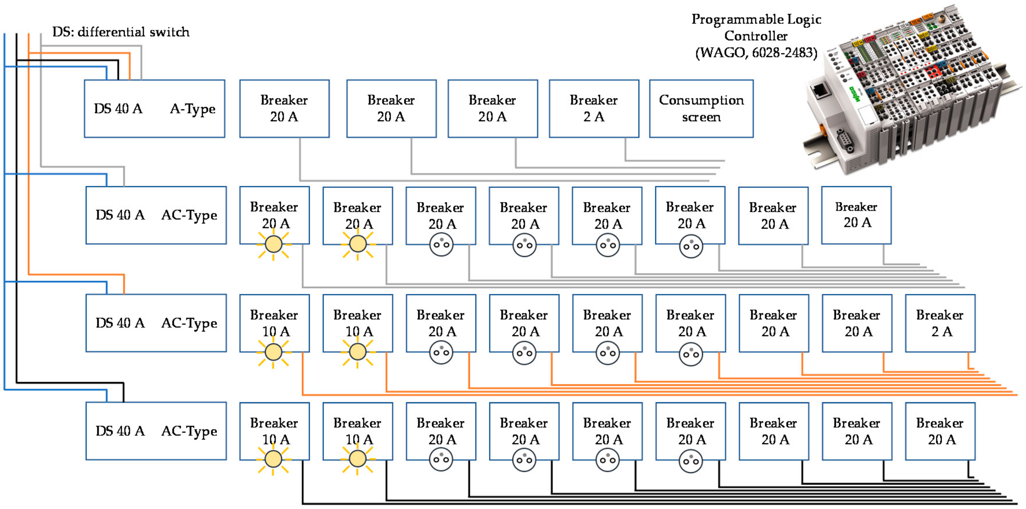
All consumption and temperature data used in this paper were obtained with a programmable logic controller (PLC) from the manufacturer named WAGO.
The PLC is used to build a database of real load electricity consumption. It was mainly chosen because of its modularity. Each module can independently be reconfigured. To carry out the experimental measurements, the PLC is composed of:
- Nine power measuring 3-phase terminals.
- One terminal with four 24 V dc input digital channels.
In order to get complete temperature databases, three acquisition modules are used. One temperature sensor is located in the bedroom, one is positioned in the living room, and the last one is located outside the house.
To build a model of each load, knowledge of load-per-load consumption is of utmost importance. Figure 2 shows how the connections were made to measure the electricity consumption.
2.2.2. Electricity Consumption Monitoring in Reference Houses
Five dwellings were monitored to build a complete database of load electricity consumption. Table 1 gives the mean features of the houses. In all instrumented houses, electricity is provided by the largest electricity supplier in France. It is important to note that consumption depends on the season of the experimentation. For example, from Table 1, 89% of the consumption of the house No. 1 is due to electric heating which is not used over the summer period.
Flexible loads, such as washing machine, dryer, dishwasher, electric heater, fridge, and oven, are defined by the users. The degree of load flexibility (FLR) ranges from 12% to 93%. The flexible power demand is calculated as shown in Equation (1).
- N: Number of samples.
- : Real power demand for time t (W).
- : Flexible power demand for time t (W).
- : Cost of electricity (Euros).
- N: Number of sampling.
- : Real power demand for time t (W).
- : Duration between two samples (s).
- : Cost of the electricity at time t (Euros/kWh).
Without the electric heating, the load flexibility rate decreases significantly. For example, from Table 2, for the first reference house (house type No. 1), this ratio decreases from 93% to 4%. This is mainly due to the heating mode i.e., electric heating, which represents 89% of the global consumption.
2.3. Load Curve Modeling
2.3.1. Methodology
A load curve is a graphical representation of an electrical variable as a function of time. In this paper, real curves are measured thanks to the system presented above. The power (in watts) is measured each minute on various loads. The aim of this study is to extract a model for each load. These models are of utmost importance to better optimize electrical energy consumption. Two examples are expressly given in the next paragraphs: a fridge and a washing machine.
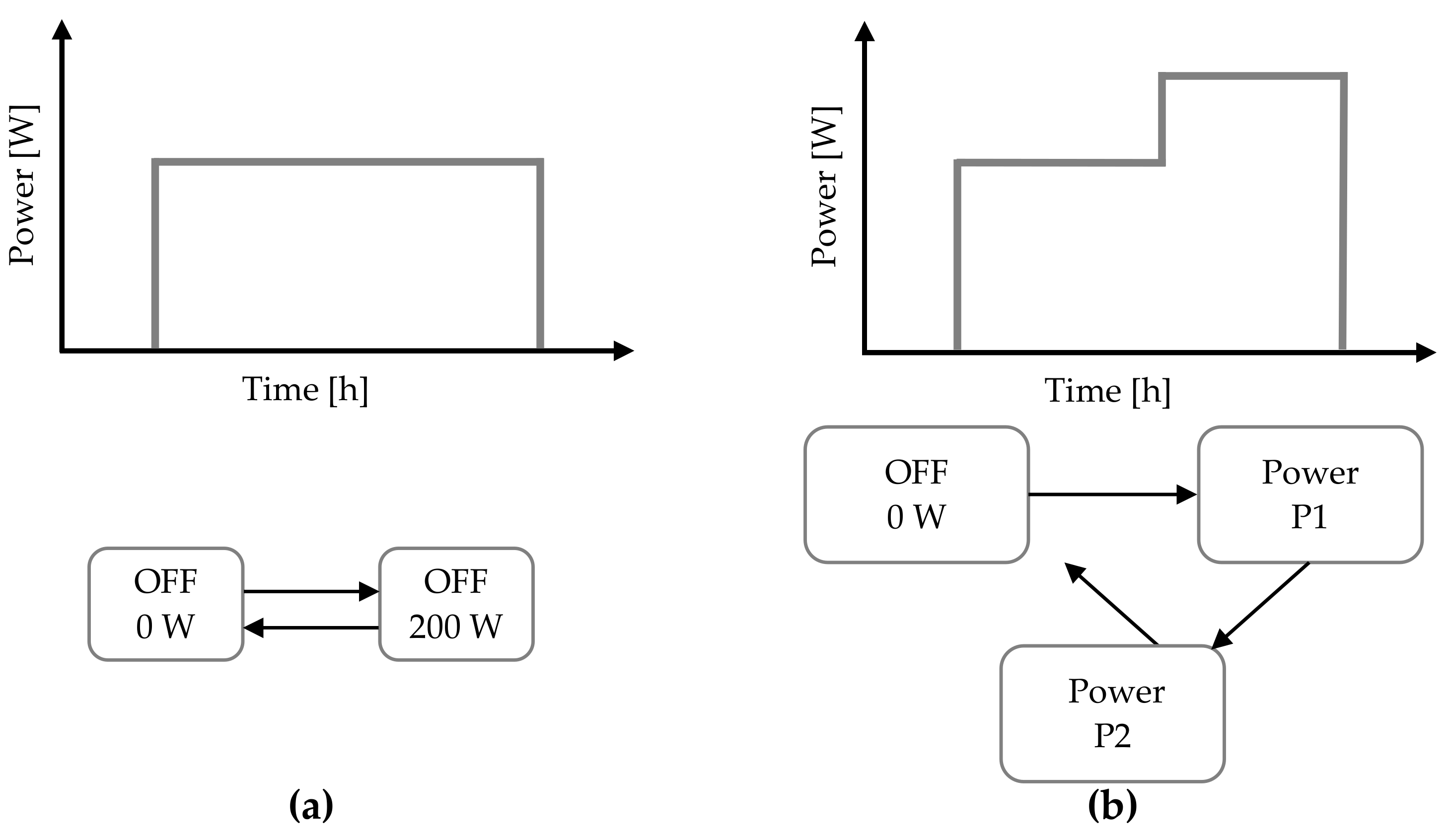
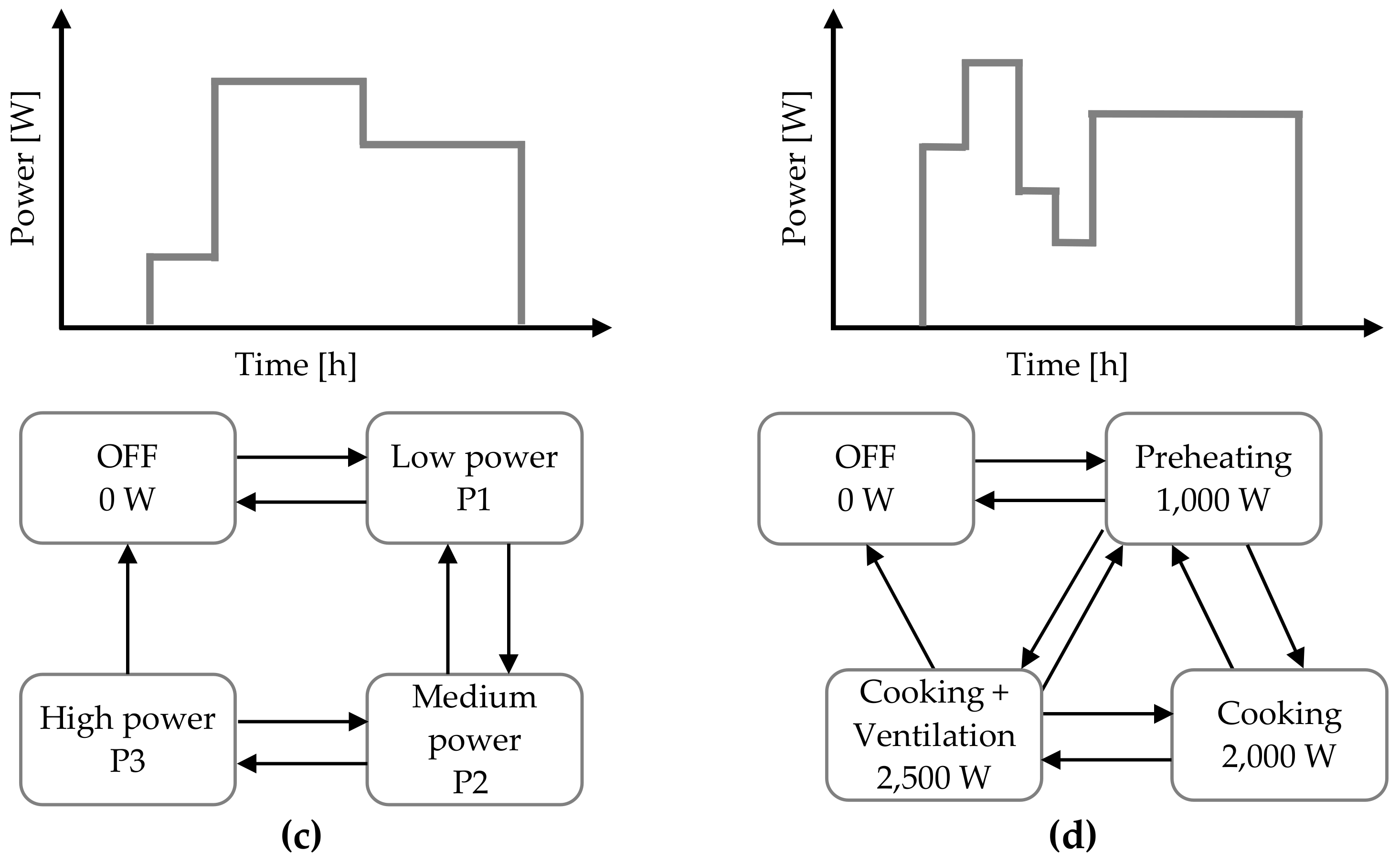
An important objective to manage any household appliance is to get a better understanding both of its consumption profile, and capacity to change (shiftable, interruptible or neither one). As can be seen in Figure 3, the procedure for identifying models may depend on the category of the device:
- Cycle and time-limited operation.
- Continuous cycle operation (type ON/OFF).
- No cycle (Computer, TV etc.).
Cycle and time-limited operations can easily be shiftable in time, but they cannot be considered as interruptible. Continuous cycle operation can also be shiftable and interruptible, but with a narrow range. Finally, devices which have no cycle are shiftable and interruptible.
2.3.2. Example of Modeling for a Fridge
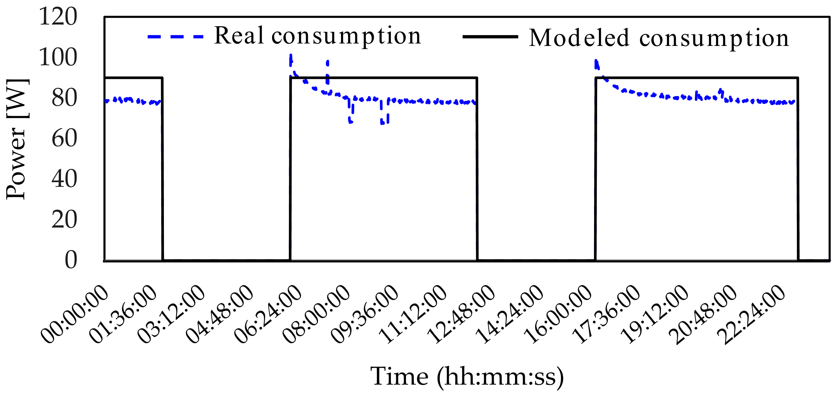
The first kind of load studied is a fridge which is an on/off operating load as shown in Figure 4. This kind of load operates typically during a period of 3 h (called on-period), and shuts down during 4 h (off-period). Its curve can so be modeled by a squared signal. The on and off-periods depend on the fridge model, its thermal insulation (if someone opens it) etc. Measurements give the necessary information to classify the fridge electricity consumption as a continuous cycle. As described previously, continuous cycle operation can be shiftable and interruptible, but with a narrow range. The fridge can be disconnected from the grid, but only for a few minutes because of its internal temperature which must be maintained at a low temperature. The off-duration depends on the manufacturer because of the quality of the thermal insulation.
2.3.3. Example of Modeling for a Washing Machine
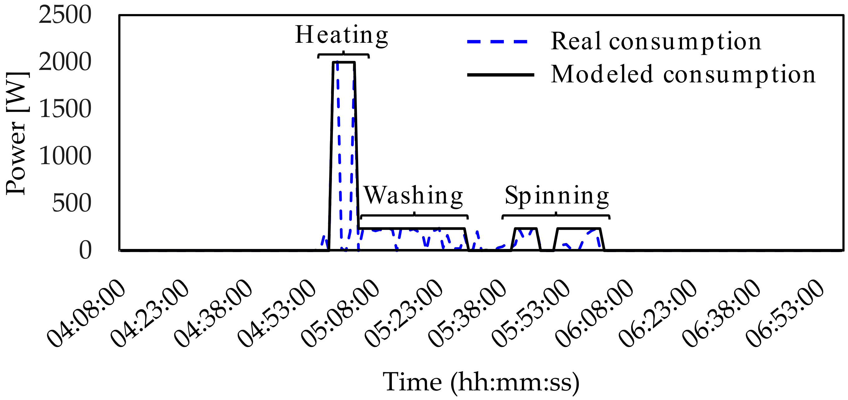
The power demand of a washing machine is shown in Figure 5. In terms of electricity consumption, this load has a cyclic behavior. Its operation depends on three elements: a drum, a heating resistance, and a pump. So, its load curve is composed of three parts. The first one is the consumption of the heating resistance necessary to heat the water. The second one represents the pump operation during the rinse cycle. The last one represents the influence of the spin cycle.
Many experimental measurements allowed the behavior of the washing machine energy consumption to be classified as a cycle and time-limited operation. This kind of power demand can easily be shiftable in time, but it is not interruptible. Therefore, to save money, it is important to shift the washing machine to start up in off-peak time. However, from Figure 5, the first cycle requires a power higher than 2000 W. So, the washing machine startup must be performed in a smart way because of the high-power demand at the beginning of the washing cycle.
2.3.4. The Importance of Sampling
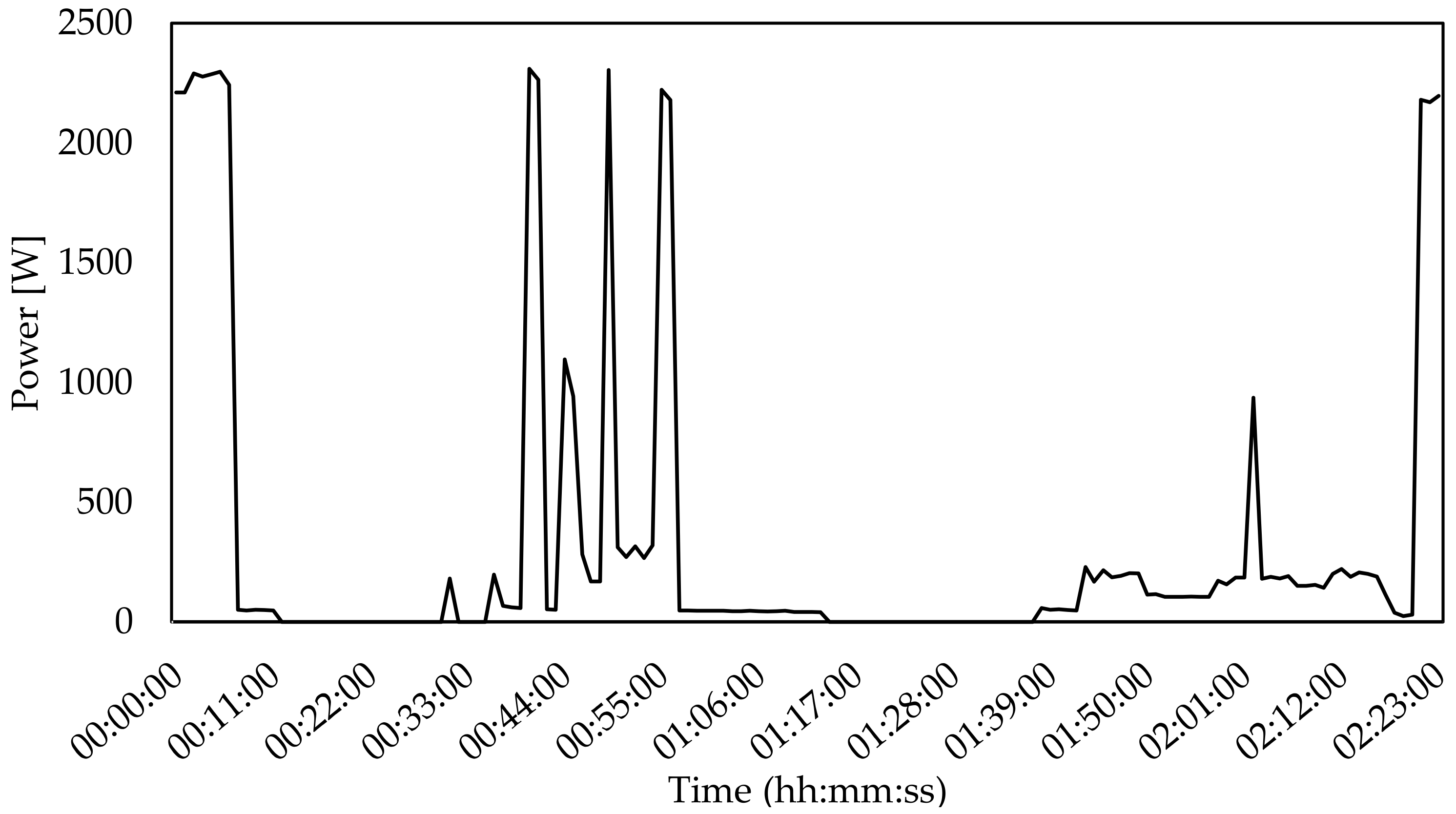
One of the most important parameters to be optimized is the sampling period. Many experiments highlighted that a sampling period of 10 min leads to an estimated electricity consumption higher than 5% in comparison with a sampling period equal to 1 min (see Figure 6 and Figure 7). This error in the prediction could be acceptable. However, with a sampling period of 10 min, a few spikes in power demand are not visible. So, it may be difficult to characterize accurately the profile of the power demand. This is the reason why a sampling period of 1 min was chosen.
3. Short Term Prediction of Load Consumption
3.1. Foreword
The strategic part of the electricity management system proposed in this article is the electricity consumption prediction that enables the quantity of harvested energy to be increased. Load forecasting has always played an important role in the planning operation. Artificial intelligence techniques are used in the prediction system. In load forecasting, the prediction is typically divided into short term load forecasting (STLF), medium term load forecasting (MTLF), and long term load forecasting (LTLF) [21,22,23]. LTLF is widely used today to decide when it is necessary to upgrade existing electricity distribution systems and build new lines or substations. MTLF is intended to predict the power demand in advance for a few weeks or months. It is mostly used to predict seasonal changes. STLF is useful to provide information to the electricity management system on day-to-day or hour-to-hour operations.
Nowadays, STLF has an important place in many operations such as real-time generation control (to balance supply and demand), security of the distribution system, and energy transaction scheduling. That is the reason why, this method was chosen to build the prediction model.
3.2. Main Inputs to Build the Prediction Model
Most prediction models have several inputs, such as the position of the day (weekday/weekend/holyday, month and/or season), temperatures, and load databases [24].
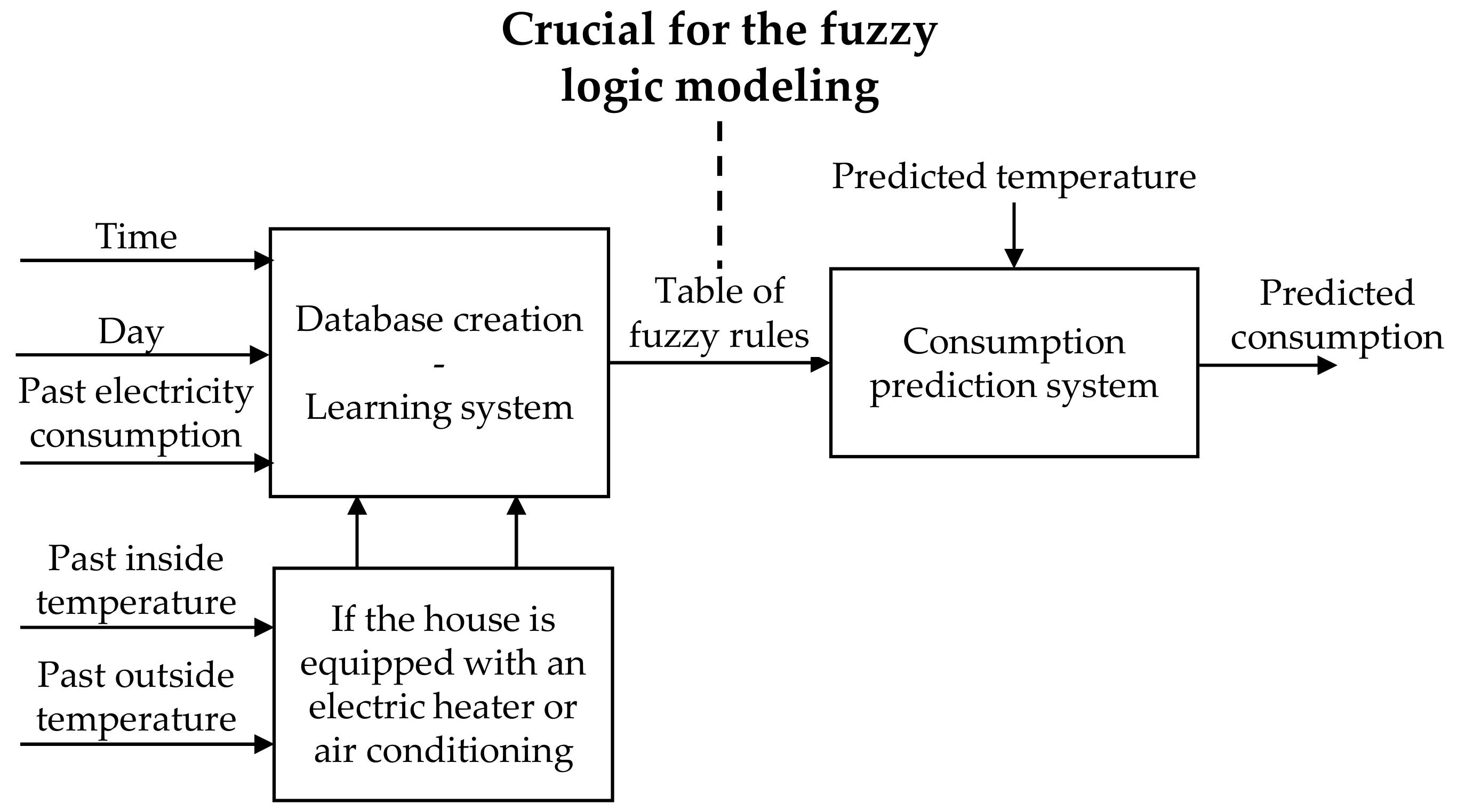
The accuracy of the prediction model relies not only on the method used to calculate the load consumption, but also the inputs. As can be seen in Figure 8, the prediction system is composed of six main inputs: day, time, past electricity consumption, past inside and outside temperatures, and predicted temperatures. In the next paragraphs, the importance of these inputs is expressly discussed.
3.2.1. Input 1: Time
The most important input is time. As can be seen in Figure 9, the power demand changes most obviously during the day. In most cases, two peak demands are particularly visible. The first one occurs during the morning between 7 a.m. and 8 a.m. The second one happens at the end of the day between 5 p.m. and 7 p.m.
3.2.2. Input 2: Day
For most people, the week is divided into two parts. The first one begins usually on Monday, and ends on Friday. The second one is the week-end from Saturday to Sunday. The experimental measurements exhibited that users’ habits do not change daily during the first part of the week. However, the energy consumption between week and weekend is rarely the same. That is the reason why the prediction system divides the week into two parts (see Figure 10).
3.2.3. Input 3: Past Electricity Consumption
The global consumption of a house is typically composed of two parts: a constant energy consumption, and a variable one. The constant part is due to standby losses (e.g., TV decoder, internet box, etc.). Therefore, it may be estimated knowing all appliances connected to the grid for the dwelling. The variable electricity consumption is more difficult to calculate. Indeed, it depends on the users’ habits (for instance, the start of the vacuum cleaner or the oven etc.).
As a consequence, a learning phase is essential. It means that a complete database of experimental measurements is mandatory to better anticipate users’ habits. The more the measurement database is refined, the more the prediction system is aware of users’ habits.
3.2.4. Inputs 4 and 5: Past Temperatures
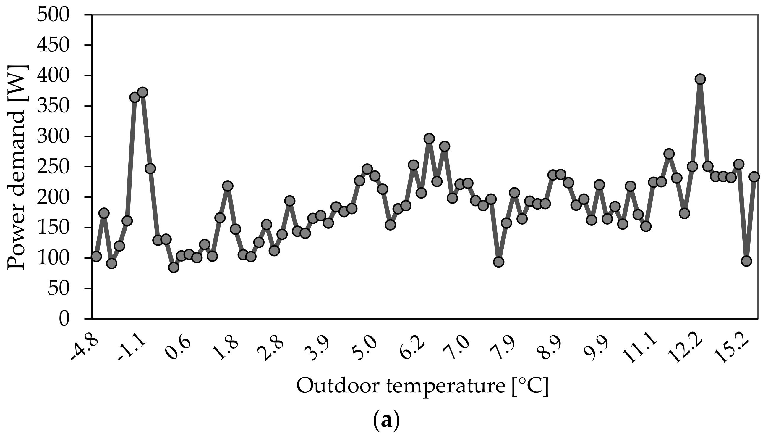
Another important input is the difference between the inside temperature and the outside one. The experimental measurements were carried out particularly to extract the relationship between the electricity consumption of a house, and the outdoor-indoor temperature mismatch. As can be seen in Figure 11a, the electricity consumption of a house without electric heaters does not depend on the temperature mismatch. Figure 11b gives the electricity consumption of a house equipped with electric heaters. A complete campaign of experimental measurements was carried out in 10 dwellings. In these 10 instrumented houses, seven were equipped with electric heaters and 40% to 80% of the electricity consumption is due to electric heating. This campaign demonstrated a significant difference in power demand between dwellings equipped with electric heaters, and those without electric heating. In all cases, a strong temperature dependence of the power demand was visible.
3.2.5. Input 6: Predicted Temperature
To better predict the electricity consumption, the modeling requires to know the indoor and outdoor temperatures for the forecasted day. For the outdoor temperature, the prediction system is connected to a statistical tool dedicated to climatology (for example, “meteo France”), and downloads the appropriate databases. For the indoor temperature, there are two possibilities as described in Equation (3).
3.3. The Fuzzy Logic as a Versatile Method Used to Predict Electricity Consumption
Existing prediction models use typically mathematical models, such as artificial neural networks (ANN), auto regressive integrated moving average (ARIMA), fuzzy neural network, time series, or advanced wavelet neural network (AWNN) [25,26,27,28,29]. Many operations such as electricity generation control, energy planning, and security studies are based on STLF. Table 3 gives particularly a comparison between the ANN, ARIMA, and fuzzy logic methods used for STLF [30,31,32,33,34,35,36]. A review of literature highlights that the fuzzy logic approach is both sufficiently efficient and versatile to meet the expectations defined at the beginning of the article. Indeed, mathematical models meet a major obstacle in the prediction of load consumption because of the non-linear relationships between the inputs (past load, past and predicted temperatures) and the output (predicted load). Such methods are also usually computationally expensive, many convergence issues are reported in the literature.
Figure 12 gives an example of fuzzy logic implementation. The definition of fuzzy rules is an important part to optimize the prediction. The fuzzy logic method offers a new approach with a logic table composed of “If-Then” rules, such as “If temperature is low”, then “electricity consumption is high”. The fuzzy logic method appears to be a great way to predict electricity consumption, because human behavior can be considered as random, and at the same time, foreseeable.
The prediction system based on the fuzzy logic method is composed of the following steps:
- The fuzzification used to convert the digital inputs into fuzzy inputs.
- The fuzzy rules necessary to stem from a learning phase to get a better understanding of the users’ habits.
- The fuzzy inference which uses the table of rules to find the electricity consumption.
- The defuzzification used to convert the fuzzy values into digital values.
One key element of the fuzzy logic approach is the definition of the membership functions. As can be seen in Figure 13, one example is given for the first input (i.e., time). From the experimental procedure, it is possible to get a complete database of the electricity consumption for the main electric devices in individual housing. From this database, it is possible to extract the mean useful duration in most appliances. In particular, it appears that most of the useful durations were a multiple of 30 min. So, time (the first input of the model) is divided into 48 triangular functions (each one lasts 30 min).
Using the same method as described above, the other inputs are divided into:
- Input 2 (day): two intervals (trapezoidal membership functions).
- Input 3 (past electricity consumption): 299 intervals (triangular membership functions).
- Input 4 and 5 (past temperatures): eight intervals (trapezoidal membership functions).
- Input 6 (predicted temperature): eight intervals (trapezoidal membership functions).
The more the number of intervals is high, the more the users’ habits are taken into consideration, whatever the inputs. Several simulation results highlighted that the accuracy of the prediction modeling can particularly be improved by changing the number of intervals for input 2 (day). The strategy consists of optimizing the division of input 2 based on a complete study of human behavior. When its membership functions are divided into seven parts (it means that each day is considered independently), the users’ habits are better taken into consideration. However, a measurement period of at least three weeks is mandatory to build an exploitable database. When the membership functions are composed of two intervals, a database of one week is satisfactory.
To illustrate what this means, the root mean square error (RMSE) is defined (see Equations (4) and (5)). This parameter is frequently used to measure the differences between values predicted by the modeling and real values (i.e., from a measurement procedure). Figure 14 shows that the RMSE-parameter decreases when the membership functions of the second input (day) are composed of two parts instead of seven parts.
- : Prediction error for time t.
- : Real power demand for time t.
- : Predicted power demand for time t.
- N: Number of samples.
Regarding the fuzzy logic diagram (see Figure 12), another important step consists of determining the fuzzy rules. Those rules, which are involved in the fuzzification and defuzzification processes, are defined during the learning period. The split of the input 1 (time), input 2 (day), and inputs 3 and 4 (temperature mismatch) into 48 intervals, 7 intervals, and 8 intervals respectively leads to 2688 possibilities. So, the table of rules is composed of 2688 h/Day/ combinations. The rules are stored in terms of “If-Then” rules such as:
- If ( is “LM”) and (DAY is “WEEK”) and (TIME is “H10”), then (Load is “LOW140”).
- If ( is “MHNM”) and (DAY is “WEEKEND”) and (TIME is “H10”), then (Load is “HIGH52”).
For each input, the more the number of interval is high, the more the prediction is accurate. Due to the increase of fuzzy rules’ possibilities, the increase of membership functions leads to the increase of Hour/Day/ combinations. The more the number of combinations is important, the more the duration to meet an acceptable prediction (i.e., error rate less than 5%) is important. However, the number of membership functions does not change the computation time. Conversely, as can be seen in Equation (6), this calculation time depends directly on the number of days.
3.4. Relevance of the Fuzzy Logic Approach : Example of Results
Figure 15 gives an example of prediction result for the house No. 1. In this case, the sampling period was equal to 1 min. The power demand was calculated for 1 day. During this period of time, the real electrical energy consumption and the modeled one are about 42.3 kWh and 38.2 kWh, respectively. So, the prediction results are very close to the measurements. It is important to note that the prediction algorithm is based on the estimation of an average consumption. Using the model, it is possible to predict the peak demand of a few loads such as water heaters, because these kinds of loads operate at the same time each day. However, regarding on/off behaviors such as heaters, the peak demand cannot easily be predicted, because their operation is directly in relation to the temperature mismatch.
4. Energy Management: Examples of Results and Discussion
4.1. New HEM Algorithm Proposal
In the previous section, the prediction algorithm based on the fuzzy logic approach enabled to better identify the users’ habits in terms of average electricity consumption. Regarding the simplified schematic of the smart home (see Figure 1), it is now very important to define the best way to use the storage system. In particular, its role is first and foremost to smooth peak demand. As a consequence, an efficient energy management algorithm is mandatory.
At the moment, HEMS plays an important role in response to the global warming effect. Since its first use in 1976, the topic has been widely discussed both in higher education and by companies [37]. Any energy management system can be achieved at the global, national, residential, or tertiary level. Today, the global and national management systems are greatly developed. The residential area is a growing market segment, particularly because of the increase of the level of pricing by the electricity suppliers. So, a smart electrical energy management system can offer a significant advantage today. New systems and technologies for home automation represent two key elements to support the development of an energy management system [38].
The HEMS enables optimal use of electricity to be defined, and helps both to reduce peak demand, and users’ electricity bills [15,39]. Numerous HEMSs are reported in the literature. They are based on existing algorithms. Most basic management systems are built to shift the consumption during off-peak time through the control of a storage system. Figure 16 gives an example of a basic flowchart [38].
In this section of the paper, a HEMS with the prediction of electricity consumption is compared with a HEMS without any prediction system. In particular, a new algorithm is discussed.
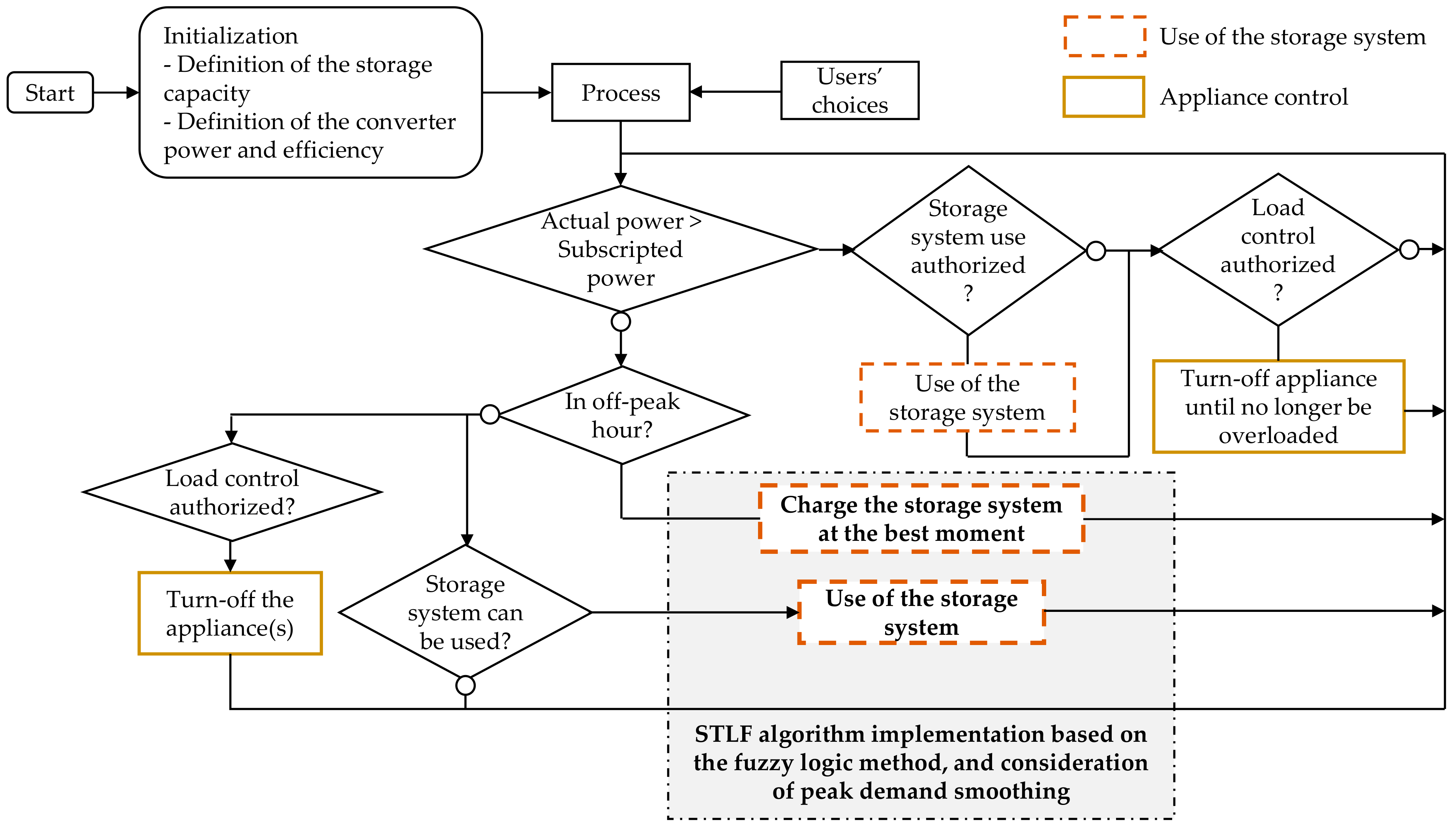
Figure 17 gives the simplified flow chart of the new algorithm. The proposed system is based on the management of the storage system in an efficient way, and the possibility to turn on/off appliances to save electricity and consequently, to decrease the cost of electricity consumption. In comparison with a basic approach, one key element of the proposed HEMS is the use of the prediction of electricity consumption based on the fuzzy logic method. Thanks to this methodology, it is possible to combine electricity savings, and the decrease of peak demand.
From a literature review, Equation (7) gives an example of the formula used to calculate the cost of electricity consumption (Ec) [40]. The aim of the algorithm is to get a better understanding of the way to reduce the Ec-parameter. The influence of the shifting of the appliances’ operation is taken into consideration by the -parameter (see Equation (8)).
- : Cost of the electricity consumption (Euros).
- : Cost of the electricity at time named t (Euros).
- . : Number of samples.
- : Efficiency of the storage system.
- . : Duration between 2 points (s).
From Equation (8), the , , and -parameters are directly linked with the classification of the appliances. In particular, these parameters represent inflexible, night, and flexible loads, respectively. Table 4 gives an example of such a classification. The flexible loads depend on the users’ choices. The users are encouraged to use night loads, i.e., during off-peak time (from 11 p.m. to 7 a.m.). The users can also choose inflexible appliances not to ensure any shifting. In the following sections, the efficiency of the storage system ( and its converter is supposed to be equal to 95%.
To better fit in with the users’ preference, it is possible to configure the system using three inputs:
- The discomfort (Dis) from 0 (0%) to 0.5 (100%).
- The use of the storage system (Su) from 0 (0%) to 0.5 (100%).
- The savings (Cs) from 0 (0%) to 1 (100%).
Equation (9) gives the relationship between these three inputs. In particular, this equation highlights that the more the discomfort and the use of the storage are important, the greater the savings are:
4.2. Examples of Simulation Results
The management strategy may be divided into two parts. The first one is dedicated to the control of the loads. The second one deals with the use of the storage system in an efficient way. Both cases are described in this section of the manuscript.
4.2.1. Smart Control of the Loads
One of the possibilities to avoid electricity waste is to optimize the operation of electric heaters. One example may consist in stopping such electrical devices during the 15 min before the off-peak period. Figure 18 gives an example of a simulation result. It is important to remember that the behavior of such heating systems strongly depends on the outdoor-indoor temperature mismatch. This switch off duration does not disturb significantly the users, because the temperature mismatch decrease is not so important.
A second possibility to avoid electricity waste may consist of shifting the electricity consumption in off-peak time. For example, it is possible to postpone the start of some electrical appliances using a smart plug. In particular, as can be seen in Figure 19, the aim is to start the devices at appropriate times to limit peak demand. When those electrical appliances cannot be equipped with any smart plug, the manufacturers of the equipment offer most often the possibility to activate an option to shift the start-up. The benefits are obviously the same.
For instance, based on a literature review, it is possible to estimate the cost savings (see Table 5) after a smart control of a few loads from their average consumption [41]:
- 288 kWh/year for a dishwasher.
- 192 kWh/year for a tumble dryer.
- 173 kWh/year for a washing machine (A+++-type).
4.2.2. Use of the Storage System in an Efficient Way
A new approach is proposed here to control the storage system in an efficient way. In this section of this paper, a new method is described to better manage electricity consumption using the predictive modeling based on the fuzzy logic approach. In the following simulations, a house with three inhabitants was considered (home No. 1).
An example of electricity consumption of this house is shown in Figure 20. When the power demand was higher than 2.6 kW, it was arbitrarily considered as a peak demand. From Figure 20, and considering the assumption described previously, 269 peaks of consumption are visible. The storage system must so be controlled in an efficient way so as to smooth those peaks.
4.3. Discussion
From the various simulation results, the proposed HEM algorithm, which implements the STLF approach based on a fuzzy logic algorithm, highlights the possibility both to optimize electricity waste, and decrease the peak demand in a significant manner. In the latter case, the efficient control of a storage system is of utmost importance both to smooth the peak demand, and shift the electricity consumption.
Many simulations were carried out from the features of the first show house (see Table 1, house type No. 1). These simulations were based on a management of the electricity consumption during 1 day, 2 days, and 9 days, respectively. Table 6 exhibits the relevance of the proposed HEM algorithm in terms of electricity saving, and peak demand reduction. To illustrate the performances of such an approach, the simulation results are compared with the ones from a basic approach as described in Figure 16. From Table 6, the decrease of the peak demand is significant when an HEMS is coupled with a STLF algorithm in all simulation cases. A basic HEM algorithm does not exhibit such positive results. Regarding electricity savings, even if a basic HEM algorithm gives acceptable results, the new algorithm proposed in this manuscript clearly strengthens the expectations.
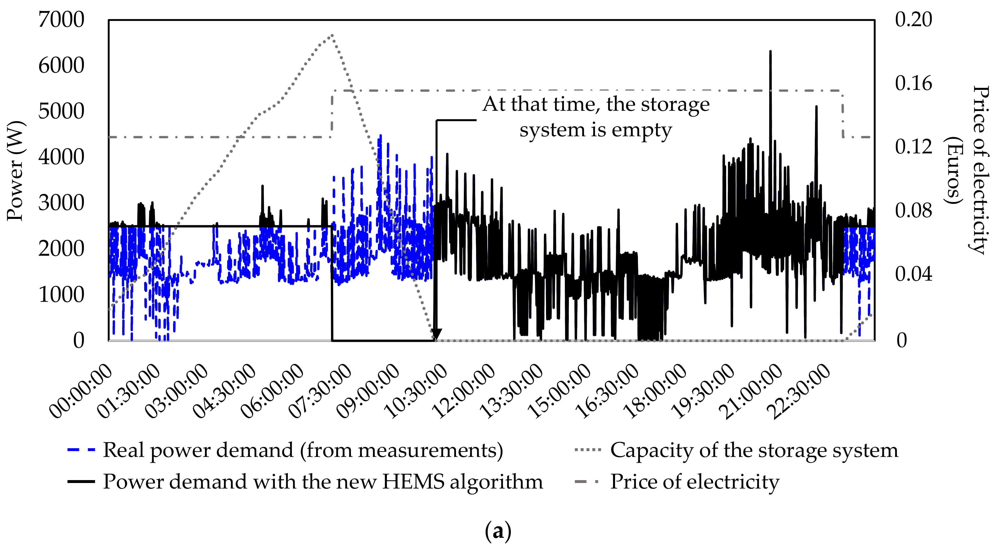
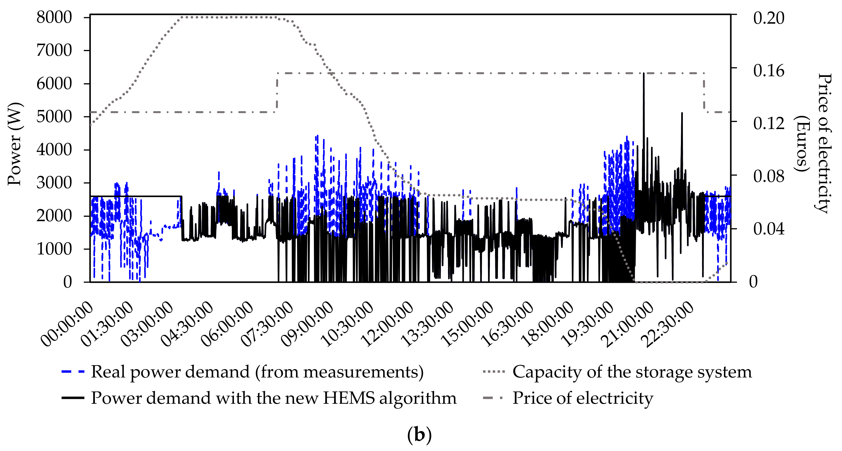
Figure 21 illustrates the impact of the control of the storage system on the management of the electricity consumption. Two cases were considered.
The first one (see Figure 21a) is based on the use of the storage system at any particular time. In particular, the storage system is charged during the peak hours (i.e., when the price of electricity is low). It is discharged without any smart control during off-peak hours (i.e., when the price of electricity is the highest). In that case, it is not possible to optimize the electricity consumption during the whole duration of the simulation because the system becomes empty very rapidly.
The second one offers the possibility to control the storage system at appropriate times through the implementation of the STLF algorithm based on the fuzzy logic method (see Figure 21b). In particular, the storage system is also charged during peak hours. However, in off-peak hours, it is progressively discharged. In that case, there are two main positive effects. The power demand of the smart house is optimized during the whole day. Moreover, most of the peak demand can be smoothed.
5. Conclusions and Prospects
This article proposed a fuzzy logic method to predict the short term load consumption in individual housing. To build the model, a complete database of real measurements was necessary. Several show houses were instrumented to meet this objective. This model represents a real cornerstone of a new algorithm used both to better manage the cost of electricity consumption in a smart home, and limit the peak demand.
The main achievements of this study are summed up below:
- The STLF algorithm based on the fuzzy logic method gave sufficient results. Many simulation results highlighted the importance of the database of real measurements to warrant an accurate prediction.
- Both simulation and experimental results highlighted the difficulty to predict STLF when a dwelling is not equipped with an electric heating.
- The electricity management system proposed in this manuscript was intended to smooth the peak demand. This can be mainly achieved using a smart control of the storage system. In particular, the HEMS allows any user to manage his energy consumption, and “reshape” the load profile. A compromise was finally highlighted between electricity waste and the reduction of the peak demand.
- The HEMS proposed in this article emphasized its strong flexibility in not disturbing the users’ comfort by scheduling home appliances.
The performances of the prediction algorithm may be improved. The existing approach is based on a day-to-day prediction. It could be interesting to take into consideration the presence of any user in the smart home to predict STLF hour by hour or minute by minute.
Acknowledgments
These research activities are currently supported by “Région Centre Val-de-Loire” (research project number: 2015-00099656). The authors of this manuscript thank our colleagues from this institution who provided insight and expertise that greatly assisted the project.
Author Contributions
Sébastien Jacques and Jean-Charles Le Bunetel organized and refined the manuscript. Sébastien Bissey conducted all the simulations and co-authored the article.
Conflicts of Interest
The authors declare no conflict of interest.
Abbreviation
The following abbreviations are used in this manuscript:
| ANN | Artificial Neural Networks |
| AP | Appliance |
| ARIMA | Auto Regressive Integrated Moving Average |
| AWNN | Advanced Wavelet Neural Network |
| FLR | Flexibility Load Range |
| HEMS | Home Energy Management System |
| LTLF | Long Term Load Forecasting |
| MTLF | Medium Term Load Forecasting |
| RMSE | Root Mean Square Error |
| STLF | Short Term Load Forecasting |
References
- U.S. Energy Information Administration. International Energy Outlook 2017; U.S. Energy Information Administration: Washington, DC, USA, 2017.
- Dynamic Pricing in Electricity Supply—A Eurelectric Position Paper. Available online: http://www.eurelectric.org/media/309103/dynamic_pricing_in_electricity_supply-2017-2520-0003-01-e.pdf (accessed on 11 February 2017).
- Mahmood, D.; Javaid, N.; Alrajeh, N.; Khan, Z.A.; Qasim, U.; Ahmed, I.; Ilahi, M. Realistic Scheduling Mechanism for Smart Homes. Energies 2016, 9, 202. [Google Scholar] [CrossRef]
- International Organization for Standardization. ISO 50001—Energy Management Systems—Requirements with Guidance for Use; International Organization for Standardization: Geneva, Switzerland, 2011. [Google Scholar]
- Laskurain, I.; Heras-Saizarbitoria, I.; Casadesús, M. Fostering renewable energy sources by standards for environmental and energy management. Renew. Sustain. Energy Rev. 2015, 50, 1148–1156. [Google Scholar] [CrossRef]
- Zobel, T.; Malmgren, C. Evaluating the Management System Approach for Industrial Energy Efficiency Improvements. Energies 2016, 9, 774. [Google Scholar] [CrossRef]
- Pau, G.; Collotta, M.; Ruano, A.; Qin, J. Smart Home Energy Management. Energies 2017, 10, 382. [Google Scholar] [CrossRef]
- Bae, H.; Yoon, J.; Lee, Y.; Lee, J.; Kim, T.; Yu, J.; Cho, S. User-friendly demand side management for smart grid networks. In Proceedings of the 2014 International Conference on Information Networking (ICOIN2014), Phuket, Thailand, 10–12 February 2014; pp. 481–485. [Google Scholar]
- Mohsenian-Rad, A.-H.; Wong, V.W.S.; Jatskevich, J.; Schober, R.; Leon-Garcia, A. Autonomous Demand-Side Management Based on Game-Theoretic Energy Consumption Scheduling for the Future Smart Grid. IEEE Trans. Smart Grid 2010, 1, 320–331. [Google Scholar] [CrossRef]
- Rodrigues, E.M.G.; Godina, R.; Shafie-khah, M.; Catalão, J.P.S. Experimental Results on a Wireless Wattmeter Device for the Integration in Home Energy Management Systems. Energies 2017, 10, 398. [Google Scholar] [CrossRef]
- Ryu, S.; Noh, J.; Kim, H. Deep Neural Network Based Demand Side Short Term Load Forecasting. Energies 2017, 10, 3. [Google Scholar] [CrossRef]
- Buitrago, J.; Asfour, S. Short-Term Forecasting of Electric Loads Using Nonlinear Autoregressive Artificial Neural Networks with Exogenous Vector Inputs. Energies 2017, 10, 40. [Google Scholar] [CrossRef]
- Hernández-Hernández, C.; Rodríguez, F.; da Costa Mendes, P.R.; Normey-Rico, J.E.; Guzmán, J.L. The Comparison Study of Short-Term Prediction Methods to Enhance the Model Predictive Controller Applied to Microgrid Energy Management. Energies 2017, 10, 884. [Google Scholar] [CrossRef]
- Zheng, H.; Yuan, J.; Chen, L. Short-Term Load Forecasting Using EMD-LSTM Neural Networks with a Xgboost Algorithm for Feature Importance Evaluation. Energies 2017, 10, 1168. [Google Scholar] [CrossRef]
- Palensky, P.; Dietrich, D. Demand Side Management: Demand Response, Intelligent Energy Systems, and Smart Loads. IEEE Trans. Ind. Inform. 2011, 7, 381–388. [Google Scholar] [CrossRef]
- Setlhaolo, D.; Xia, X. Optimal scheduling of household appliances with a battery storage system and coordination. Energy Build. 2015, 94, 61–70. [Google Scholar] [CrossRef]
- Esther, B.P.; Kumar, K.S. A survey on residential Demand Side Management architecture, approaches, optimization models and methods. Renew. Sustain. Energy Rev. 2016, 59, 342–351. [Google Scholar] [CrossRef]
- Rasheed, M.; Javaid, N.; Awais, M.; Khan, Z.; Qasim, U.; Alrajeh, N.; Iqbal, Z.; Javaid, Q. Real Time Information Based Energy Management Using Customer Preferences and Dynamic Pricing in Smart Homes. Energies 2016, 9, 542. [Google Scholar] [CrossRef]
- Dolara, A.; Grimaccia, F.; Magistrati, G.; Marchegiani, G. Optimization Models for Islanded Micro-Grids: A Comparative Analysis between Linear Programming and Mixed Integer Programming. Energies 2017, 10, 241. [Google Scholar] [CrossRef]
- Ahmad, A.; Khan, A.; Javaid, N.; Hussain, H.M.; Abdul, W.; Almogren, A.; Alamri, A.; Azim Niaz, I. An Optimized Home Energy Management System with Integrated Renewable Energy and Storage Resources. Energies 2017, 10, 549. [Google Scholar] [CrossRef]
- Ghiassi, M.; Zimbra, D.K.; Saidane, H. Medium term system load forecasting with a dynamic artificial neural network model. Electr. Power Syst. Res. 2006, 76, 302–316. [Google Scholar] [CrossRef]
- Ali, D.; Yohanna, M.; Puwu, M.I.; Garkida, B.M. Long-term load forecast modelling using a fuzzy logic approach. Pac. Sci. Rev. A Nat. Sci. Eng. 2016, 18, 123–127. [Google Scholar] [CrossRef]
- Sadaei, H.J.; Guimarães, F.G.; da Silva, C.J.; Hisyam Lee, M.; Eslami, T. Short-term load forecasting method based on fuzzy time series, seasonality and long memory process. Int. J. Approx. Reason. 2017, 83, 196–217. [Google Scholar] [CrossRef]
- Byeon, G.; Yoon, T.; Oh, S.; Jang, G. Energy Management Strategy of the DC Distribution System in Buildings Using the EV Service Model. IEEE Trans. Power Electron. 2013, 28, 1544–1554. [Google Scholar] [CrossRef]
- Rana, M.; Koprinska, I. Forecasting electricity load with advanced wavelet neural networks. Neurocomputing 2016, 182, 118–132. [Google Scholar] [CrossRef]
- Barak, S.; Sadegh, S.S. Forecasting energy consumption using ensemble ARIMA–ANFIS hybrid algorithm. Int. J. Electr. Power Energy Syst. 2016, 82, 92–104. [Google Scholar] [CrossRef]
- Liao, G.-C.; Tsao, T.-P. Application of fuzzy neural networks and artificial intelligence for load forecasting. Electr. Power Syst. Res. 2004, 70, 237–244. [Google Scholar] [CrossRef]
- Clements, A.E.; Hurn, A.S.; Li, Z. Forecasting day-ahead electricity load using a multiple equation time series approach. Eur. J. Oper. Res. 2016, 251, 522–530. [Google Scholar] [CrossRef]
- Jovanović, R.Ž.; Sretenović, A.A.; Živković, B.D. Ensemble of various neural networks for prediction of heating energy consumption. Energy Build. 2015, 94, 189–199. [Google Scholar] [CrossRef]
- Kavaklioglu, K.; Ceylan, H.; Ozturk, H.K.; Canyurt, O.E. Modeling and prediction of Turkey’s electricity consumption using Artificial Neural Networks. Energy Convers. Manag. 2009, 50, 2719–2727. [Google Scholar] [CrossRef]
- Yuce, B.; Mourshed, M.; Rezgui, Y. A Smart Forecasting Approach to District Energy Management. Energies 2017, 10, 1073. [Google Scholar]
- Pappas, S.S.; Ekonomou, L.; Karamousantas, D.C.; Chatzarakis, G.E.; Katsikas, S.K.; Liatsis, P. Electricity demand loads modeling using AutoRegressive Moving Average (ARMA) models. Energy 2008, 33, 1353–1360. [Google Scholar] [CrossRef]
- Azadeh, A.; Saberi, M.; Seraj, O. An integrated fuzzy regression algorithm for energy consumption estimation with non-stationary data: A case study of Iran. Energy 2010, 35, 2351–2366. [Google Scholar] [CrossRef]
- Chaturvedi, D.K.; Sinha, A.P.; Malik, O.P. Short term load forecast using fuzzy logic and wavelet transform integrated generalized neural network. Int. J. Electr. Power Energy Syst. 2015, 67, 230–237. [Google Scholar] [CrossRef]
- Mamlook, R.; Badran, O.; Abdulhadi, E. A fuzzy inference model for short-term load forecasting. Energy Policy 2009, 37, 1239–1248. [Google Scholar] [CrossRef]
- Castro Torrini, F.; Castro Souza, R.; Cyrino Oliveira, F.L.; Moreira Passanha, J.F. Long term electricity consumption forecast in Brazil: A fuzzy logic approach. Socioecon. Plann. Sci. 2016, 54, 18–27. [Google Scholar] [CrossRef]
- Berlad, A.L.; Salzano, F.J.; Batey, J. On enthalpy management in small buildings. Energy 1976, 1, 429–443. [Google Scholar] [CrossRef]
- Lobaccaro, G.; Carlucci, S.; Löfström, E. A Review of Systems and Technologies for Smart Homes and Smart Grids. Energies 2016, 9, 348. [Google Scholar] [CrossRef]
- Strbac, G. Demand side management: Benefits and challenges. Energy Policy 2008, 36, 4419–4426. [Google Scholar] [CrossRef]
- Setlhaolo, D.; Xia, X. Combined residential demand side management strategies with coordination and economic analysis. Int. J. Electr. Power Energy Syst. 2016, 79, 150–160. [Google Scholar] [CrossRef]
- How Much Energy Do My Household Appliances Use?—Energuide. Available online: https://www.energuide.be/en/questions-answers/how-much-energy-do-my-household-appliances-use/71/ (accessed on 11 August 2017).
Figure 1.
Simplified illustration of the proposed smart home.
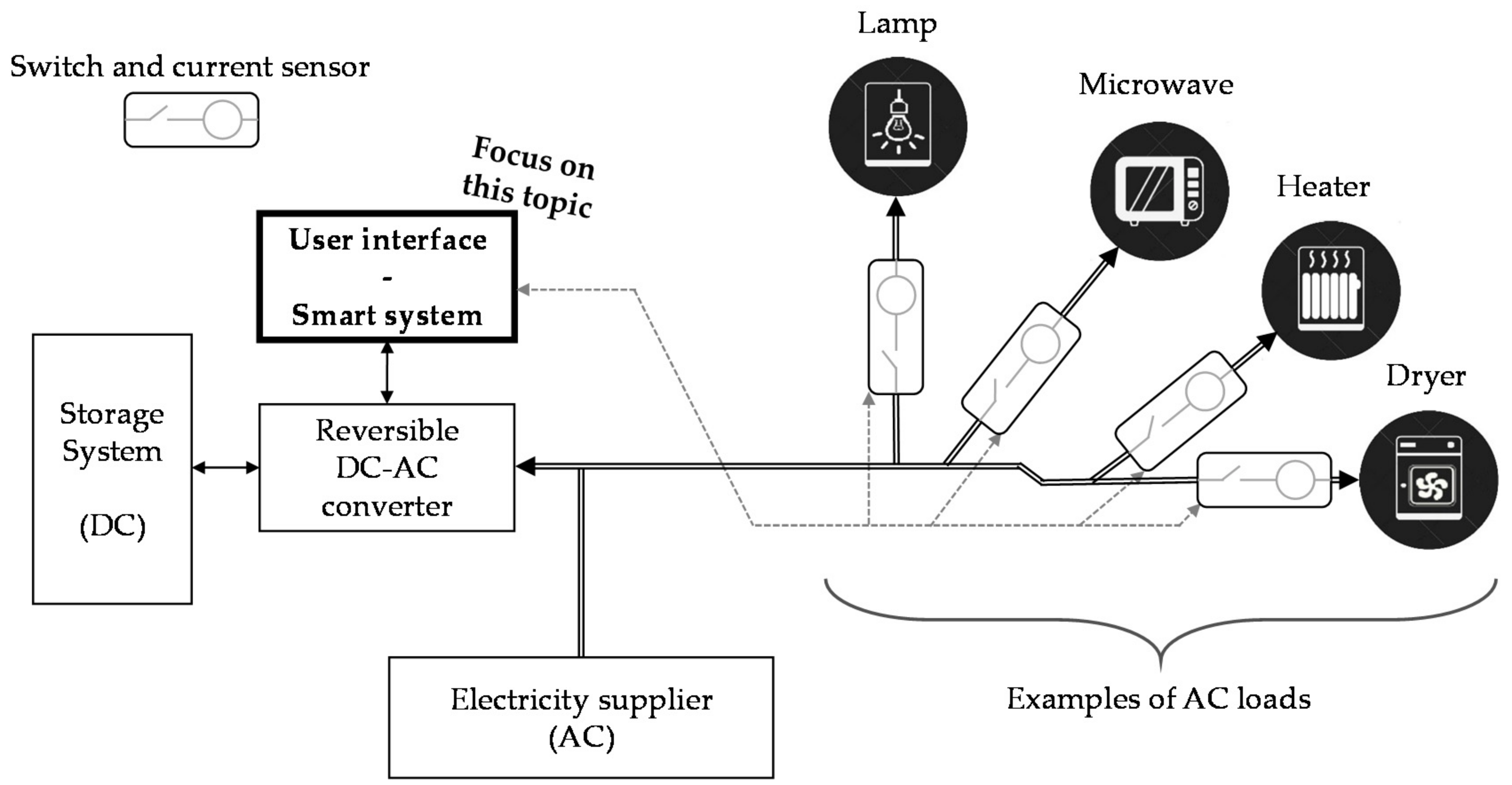
Figure 2.
Example of wiring of the measurement system in the electric panel of a smart home.

Figure 3.
Finite state models: (a) two states model e.g., electric heating, toaster; (b) two operating modes appliances, e.g., lamp; (c) multiple states appliances e.g., devices on battery (with battery in charge/loaded battery); (d) multiple states and paths, e.g., oven, washing machine, dishwasher.


Figure 4.
Example of power demand for a fridge.

Figure 5.
Example of power demand for a washing machine.

Figure 6.
Example of power demand of a house with sampling equal to 10 min.

Figure 7.
Example of power demand of a house with sampling equal to 1 min.
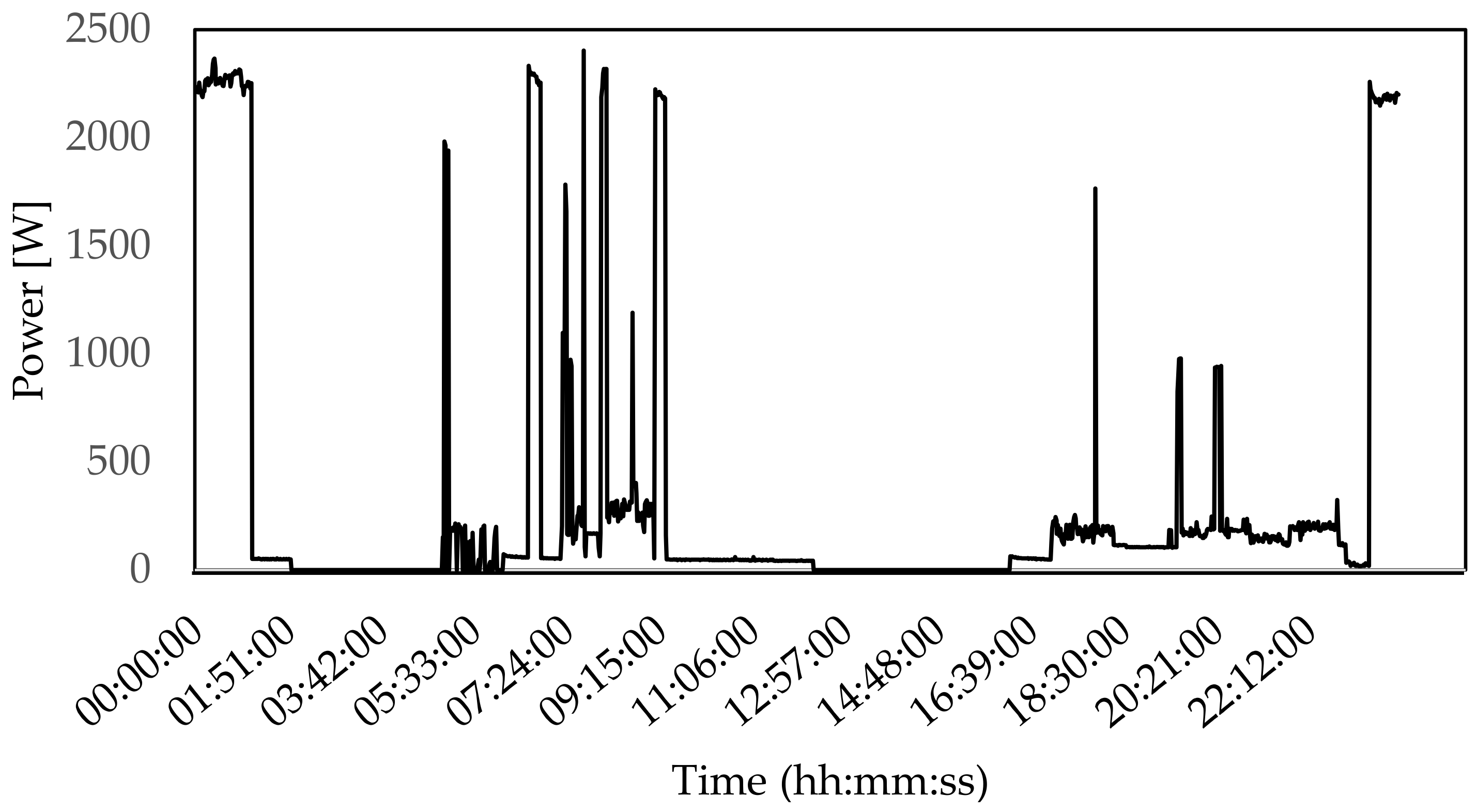
Figure 8.
Diagram of the electricity prediction system.

Figure 9.
Example of electricity demand depending on time (house with 4 inhabitants).
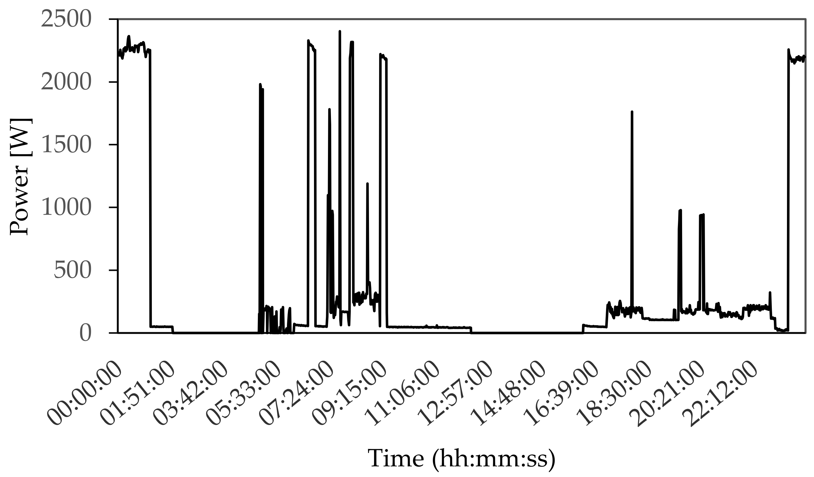
Figure 10.
Division of the input 2 (day).
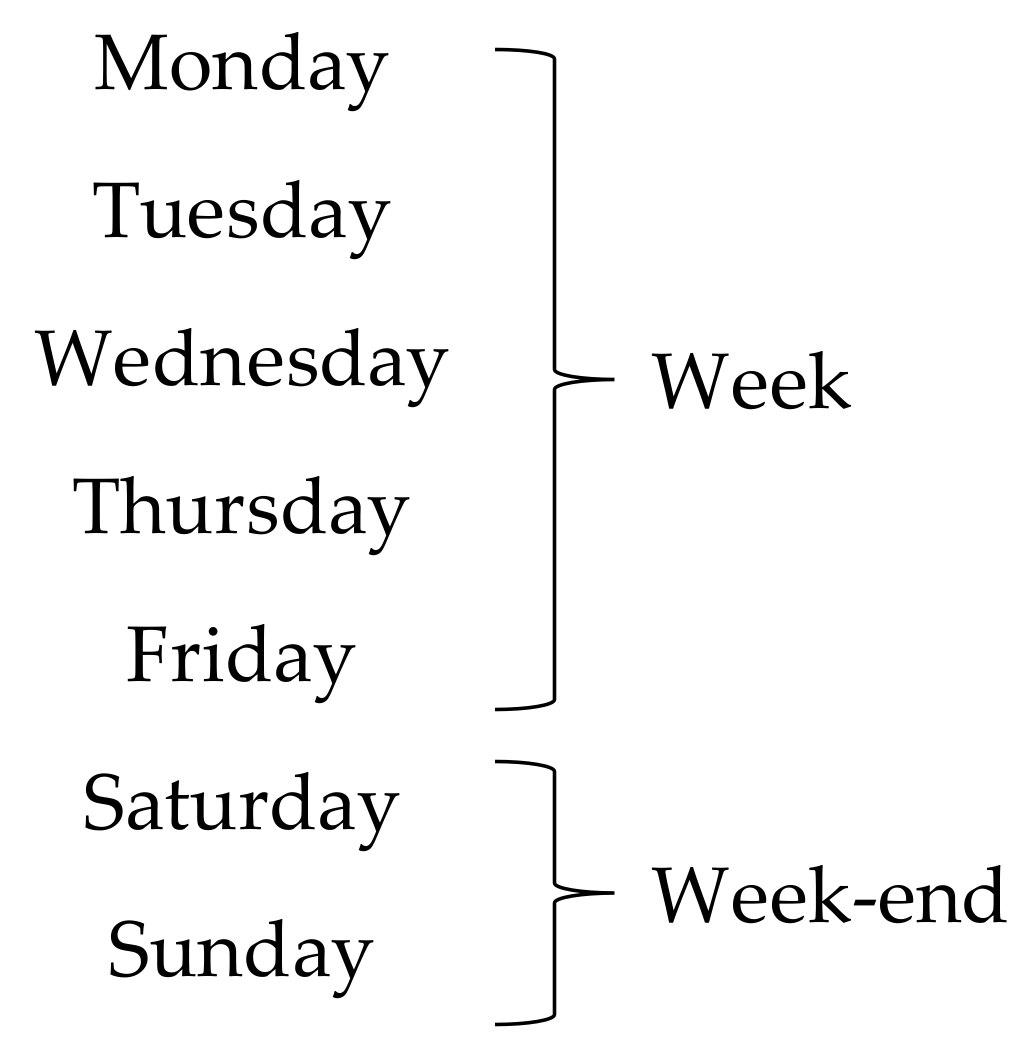
Figure 11.
Relationship between electricity demand, and the difference between the outside and inside temperatures of the house. (a) Without any electric heater. (b) With several electric heaters.
Figure 11.
Relationship between electricity demand, and the difference between the outside and inside temperatures of the house. (a) Without any electric heater. (b) With several electric heaters.

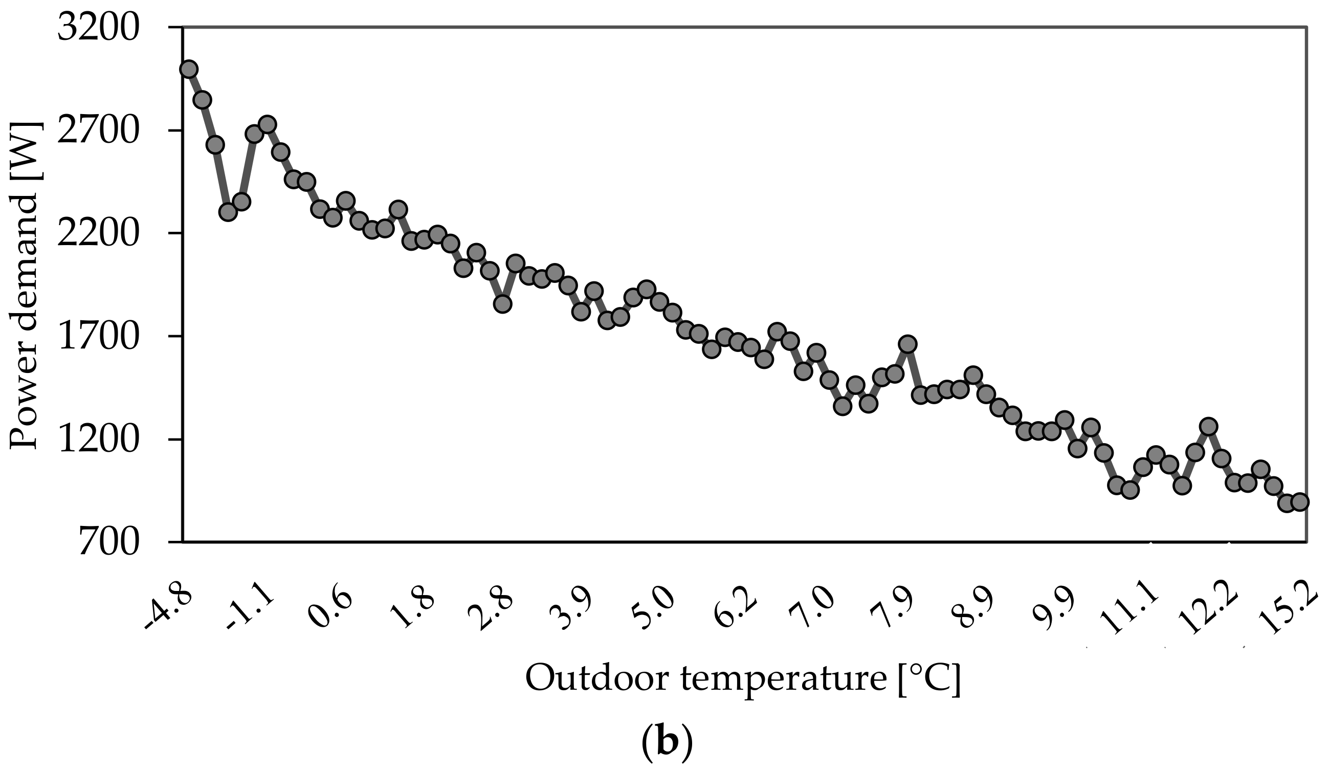
Figure 12.
Block diagram of a fuzzy logic system dedicated to STLF.
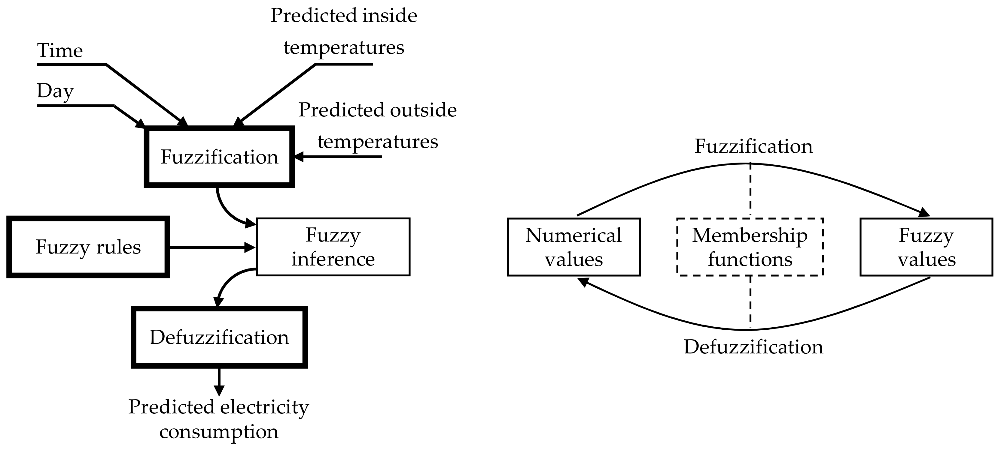
Figure 13.
Example of triangular membership functions for the first input of the model (Time).
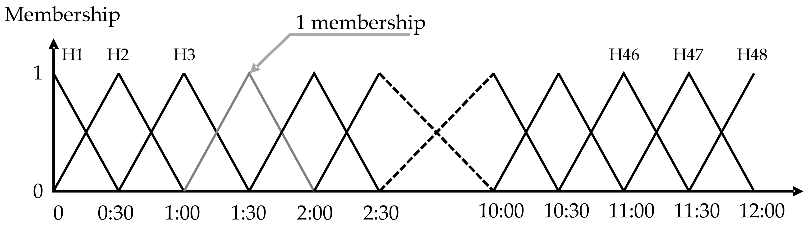
Figure 14.
Root Mean Square Error comparison for input 2 (day).
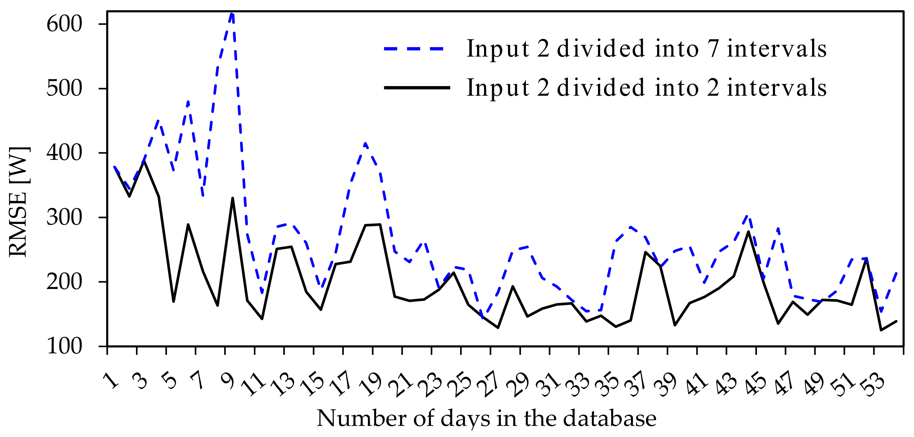
Figure 15.
Example of an electricity consumption prediction for 1 day (house No. 1, 3 inhabitants, 130 m2, electric heating, sampling period equal to 1 min).
Figure 15.
Example of an electricity consumption prediction for 1 day (house No. 1, 3 inhabitants, 130 m2, electric heating, sampling period equal to 1 min).
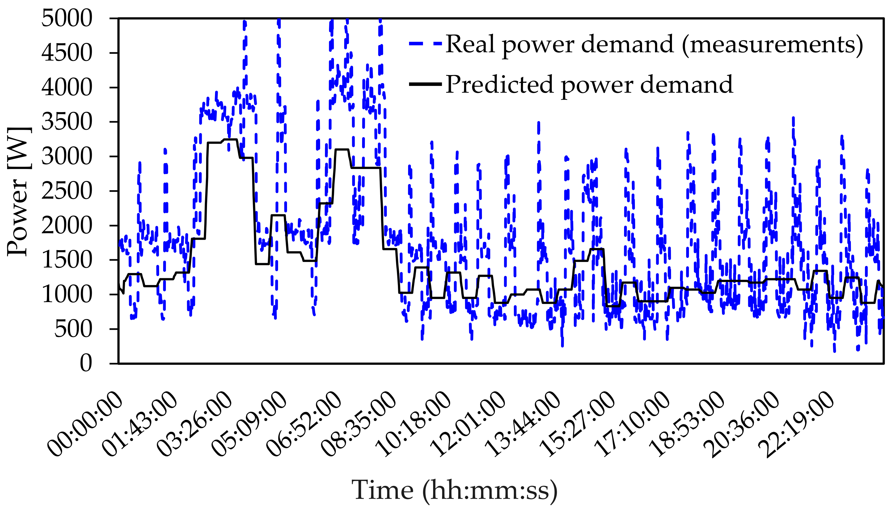
Figure 16.
Flowchart of a basic HEMS without any STLF algorithm [38].
Figure 16.
Flowchart of a basic HEMS without any STLF algorithm [38].
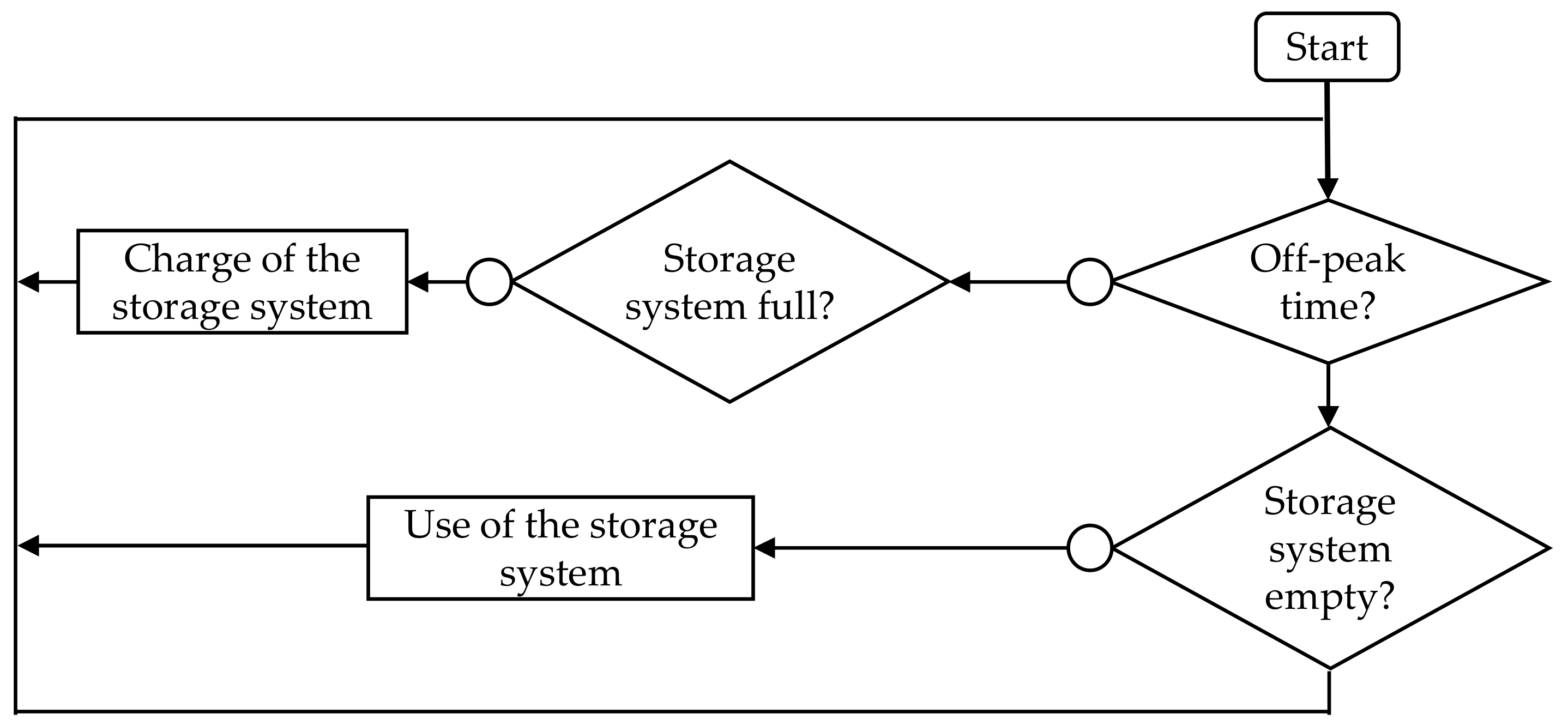
Figure 17.
Simplified flow chart of the proposed HEMS algorithm that implements both STLF and peak demand smoothing.
Figure 17.
Simplified flow chart of the proposed HEMS algorithm that implements both STLF and peak demand smoothing.

Figure 18.
Example of electricity management of an electrical heater.

Figure 19.
Example of electricity management of 2 electrical devices: real power demand (from measurements) (a). Power demand after a smart control of the loads (b).
Figure 19.
Example of electricity management of 2 electrical devices: real power demand (from measurements) (a). Power demand after a smart control of the loads (b).
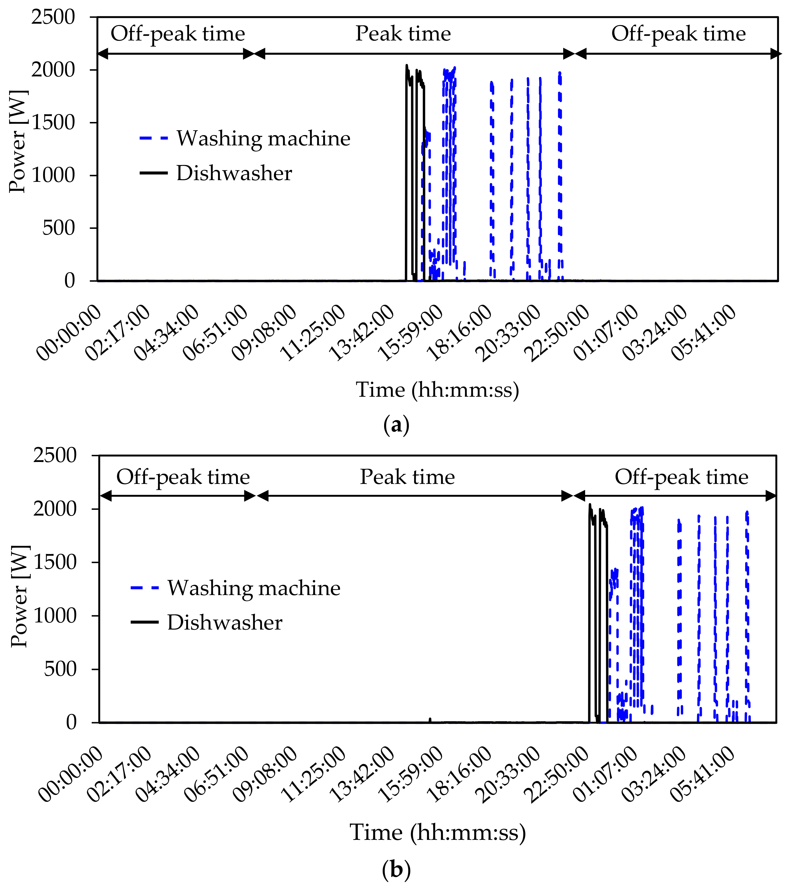
Figure 20.
Power demand for the show house No. 1 (3 inhabitants, 130 m2, electric heating, sampling period equal to 1 min).
Figure 20.
Power demand for the show house No. 1 (3 inhabitants, 130 m2, electric heating, sampling period equal to 1 min).

Figure 21.
Relevance of the proposed HEMS with an appropriate control of the storage system. Without any STLF algorithm (a). With the STLF algorithm based on the fuzzy logic method (b).
Figure 21.
Relevance of the proposed HEMS with an appropriate control of the storage system. Without any STLF algorithm (a). With the STLF algorithm based on the fuzzy logic method (b).

Table 1.
Main features of the reference houses.
| House Type No. | House Type | Surface Area (m2) | Small Appliances Consumption (Wh/Day) | Consumption of Energy-Inefficient Appliances (Wh/Day) | Monthly Invoice * (Euros) | Season of the Experimentation |
|---|---|---|---|---|---|---|
| 1 | House | 130 | 2773 | 38,190 | 170 | Winter |
| 2 | Apartment | 50 | 1701 | 2708 | 15.6 | Autumn |
| 3 | Apartment | 35 | 2566 | 6084 | 26.8 | Autumn |
| 4 | House | 100 | 3783 | 5483 | 39 | Summer |
| 5 | House | 150 | 11,942 | 45,847 | 244 | Winter |
* The monthly invoice is estimated using Equation (2).
Table 2.
Review of flexible loads in instrumented houses.
| House Type No. | Heating Mode | Load Flexibility Rate (%) | Load Flexibility Rate without Electic Heating (%) |
|---|---|---|---|
| 1 | Electric | 93 | 4 |
| 2 | Gas and electric | 12 | 8 |
| 3 | Electric | 32 | 30 |
| 4 | Gas | 25 | 25 |
| 5 | Electric | 84 | 29 |
Table 3.
Relevance of the fuzzy logic method in comparison with the ANN and ARIMA mathematical approaches.
Table 3.
Relevance of the fuzzy logic method in comparison with the ANN and ARIMA mathematical approaches.
| Model | ANN | ARIMA | Fuzzy Logic | ||||||
|---|---|---|---|---|---|---|---|---|---|
| Study | [30] | [31] | [12] | [32] | [26] | [33] | [34] | [35] | [36] |
| Prediction basis | Yearly | Daily | Daily | Daily | Yearly | Monthly | Hourly | Daily | Yearly |
| Scope of the prediction | Country (Turkey) | Country (Ireland) | Region (USA) | Country (Greece) | Country (Iran) | Country (Iran) | Substation (India) | Country (Jordan) | Country (Brazil) |
| Operating mode |
|
|
| ||||||
| Advantages |
|
|
| ||||||
| Drawbacks |
|
|
| ||||||
| Appliances | Type | Flexibility Classification | Flexibility Time (min) (Assumption) | Rated Power (kW) | Time-of-Use (Average Duration) |
|---|---|---|---|---|---|
| Washing Machine | C * | N ** | ±120 | 2.5 | 48 weeks/year—4 times a week |
| Dishwasher | C * | N ** | ±120 | 1.2 | 48 weeks/year—5 times a week |
| Dryer | C * | F ** | ±30 | 2.75 | 32 weeks/year—2 times a week |
| Fridge | C * | F ** | ±5 | 0.25 | 365 days/year |
| Electric oven | C * | F ** | ±15 | 2.25 | 48 weeks/year—1.5 h/week |
| Electric vehicle | C * | F ** | ±120 | 3 | 9 h/recharge |
| Electric heater | C * | F ** | ±30 | 1.5 | 100 kWh/year/m2 |
| Water heater | C * | F ** | ±120 | 2.2 | 365 days/year—70 min/day |
| Microwave | NC * | I ** | - | 1.25 | 48 weeks/year—1.5 h/week |
| Coffee maker | NC * | I ** | - | 0.60 | 335 days/year—10 min/day |
| Hair dryer | NC * | I ** | - | 0.5 | 48 weeks/year—30 min/day |
C *: controllable load; NC *: non-controllable load. N **: night load; F **: flexible load; I **: inflexible load.
Table 5.
Electricity cost savings: benefits of a smart management of the electricity consumption.
| Electrical Appliances | Electricity Cost without Management (Euros) | Electricity Cost with a Smart Management (Euros) | ||
|---|---|---|---|---|
| One Cycle | Annual | One Cycle | Annual | |
| Dishwasher | 0.1911 | 45.88 | 0.1502 | 36.06 |
| Tumble dryer | 0.4779 | 30.60 | 0.3756 | 24.04 |
| Washing machine (A+++-type) | 0.1434 | 27.56 | 0.1127 | 21.66 |
Table 6.
Relevance of the new HEM algorithm implementing the STLF based on the fuzzy logic method, and, at the same time, peak demand smoothing.
Table 6.
Relevance of the new HEM algorithm implementing the STLF based on the fuzzy logic method, and, at the same time, peak demand smoothing.
| Number of Days for the Simulation | Electricity Savings and Number of Peaks | Before the Management | After Basic Management without Prediction System | After Management with Prediction System |
|---|---|---|---|---|
| 1 day | Electricity savings | 0 | 17.5% | 13.5% |
| Number of peaks | 269 | 162 | 0 | |
| 2 days | Electricity savings | 0 | 11.0% | 5.0% |
| Number of peaks | 372 | 253 | 0 | |
| 9 days | Electricity savings | 0 | 5.0% | 4.3% |
| Number of peaks | 2042 | 1461 | 342 |
© 2017 by the authors. Licensee MDPI, Basel, Switzerland. This article is an open access article distributed under the terms and conditions of the Creative Commons Attribution (CC BY) license (http://creativecommons.org/licenses/by/4.0/).
Share and Cite
MDPI and ACS Style
Bissey, S.; Jacques, S.; Le Bunetel, J.-C. The Fuzzy Logic Method to Efficiently Optimize Electricity Consumption in Individual Housing. Energies 2017, 10, 1701. https://doi.org/10.3390/en10111701
AMA Style
Bissey S, Jacques S, Le Bunetel J-C. The Fuzzy Logic Method to Efficiently Optimize Electricity Consumption in Individual Housing. Energies. 2017; 10(11):1701. https://doi.org/10.3390/en10111701
Chicago/Turabian StyleBissey, Sébastien, Sébastien Jacques, and Jean-Charles Le Bunetel. 2017. "The Fuzzy Logic Method to Efficiently Optimize Electricity Consumption in Individual Housing" Energies 10, no. 11: 1701. https://doi.org/10.3390/en10111701
Note that from the first issue of 2016, this journal uses article numbers instead of page numbers. See further details here.