Pressure-Drop Coefficients for Cushioning System of Hydraulic Cylinder With Grooved Piston: A Computational Fluid Dynamic Simulation

Abstract

Cushioning is an important aspect in hydraulic cylinder performance. The piston has to be decelerated before it strikes the end cap in order to avoid stresses in the cylinder components and reduce vibration that can be transmitted to the machine. One of the least-studied methods is internal cushioning by grooves in the piston. In this method, the flow is throttled with adequately designed grooves when the piston reaches the outlet port position. The purpose of the present work is to present a method to estimate the pressure-drop coefficients for a certain design of piston grooves in order to provide a model to develop a dynamic system simulation of the cushion system. The method is based on a computational fluid dynamic simulation of flow through piston grooves to the outlet port for each piston’s static position. The results are compared with experimental measurements, and a correction, based on Reynolds number, is proposed. Good agreement, below 16%, was obtained for all the positions but particularly for the last grooves, for which the numerical result’s deviation to the experimental measurements was less than 10%. In general, the numerical simulation tended to underestimate the pressure drop for the first grooves and overestimate the calculation for the last grooves.

1. Introduction

End stroke cushioning in a hydraulic cylinder is important because it avoids mechanical shocks by reducing the piston velocity at the end of the cycle. However, the cushioning system has to be carefully designed in order to minimize the operating cycle time, allowing faster machine operating cycles for productivity increase. A proper cushioning system reduces machine noise for less downtime and lowers the machine maintenance costs [1].

Cushioning can be done with external control, but for mobile applications, this is not generally appropriate, as it requires a complex set-up of mechanical and hydraulic components [2,3]. Alternatively, in this case of mobile applications, internal end-stroke cushioning systems are preferably used.

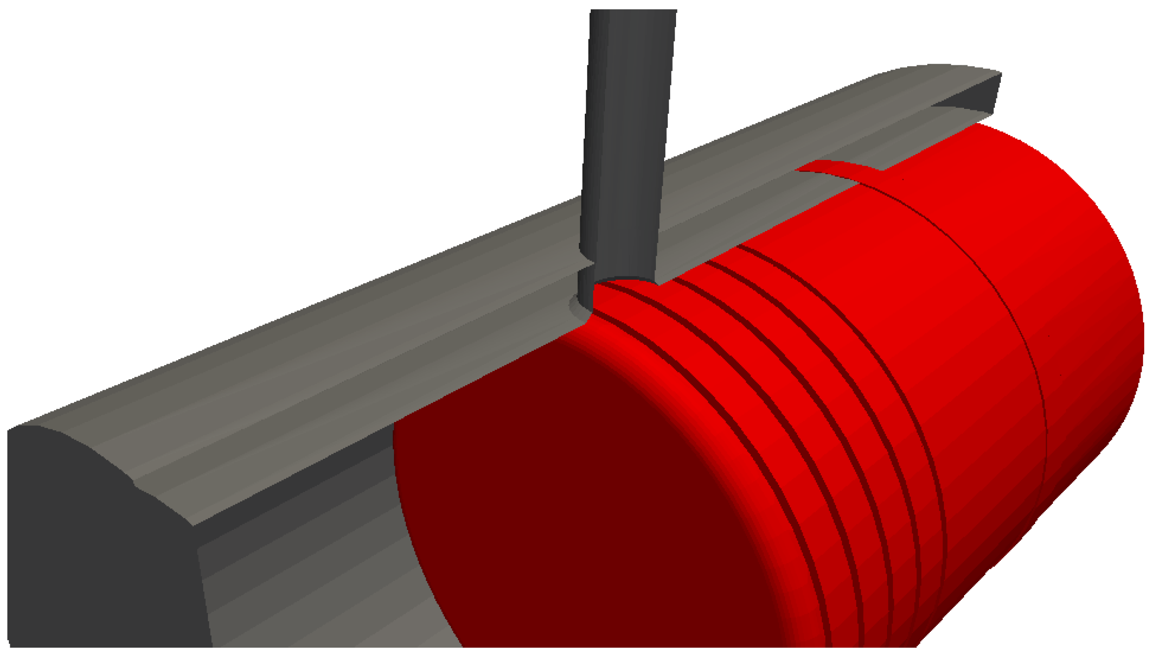
There are two main types of stroke-end hydraulic cylinder cushioning. On the one hand, it is usual to include a spear with a profile that fits conveniently in a hole drilled at the end of the cylinder. Throttling is then performed in this orifice in order to control the velocity of the piston and the pressure in the cylinder chamber. On the other hand, machining can be performed in the piston with a given number of grooves that control the oil flow rate and the pressure loss.

The first case has been extensively studied. Borgui et al. [4] present a numerical model, supported by experimental results, obtained by the analysis of a considerable number of geometries. Schwartz et al. [5] presented a similar work to Borghi et al. Both works demonstrate the complexity of the cushioning system and the sensitivity to the main geometric parameters. The recent work by Prahallad and Raveender [6] analyses different geometries used in end-stroke cushioning systems. Gao et al. [7] use the commercial simulation software of mechatronic systems AMESIM to optimize a cushioning system with a step-shaped spear.

The second type of internal cushioning, with groove machining in the piston, has not received much attention. The effect of grooves in friction reduction in pistons is well documented [8,9], but the effect on stability or cushioning performance has not been extensively studied.

Viscous flow in cylinder gaps has been thoroughly studied in the context of piston pumps. Recently, Zawistowski and Kleiber [10] made an extensive review of simulation methods in this field, remarking on the contributions of Bergada et al. [11,12] and Hao and Qi [13], who solved Reynolds equations for flow leakage in piston pumps. Ivantysynova and Huang [14] considered elastohydrodynamic effects. Similarly, the effect of grooves in the piston has been numerically analyzed from the point of view of stability in piston pumps by Khumar and Bergada [15].

Very recently, Algar et al. [16] published an experimental test of cushioning performance of a cylinder with two grooves in the piston, finding that the three dimensional piston displacement plays an important role as a self-adjusting element.

The purpose of this work is to present a method to estimate the value of the pressure-drop coefficients for the flow through piston grooves towards the outlet port. Special attention is paid to the role of eccentricity on the cushioning performance, as a result of the research reported by Algar et al. [16]. This method is aimed at providing the model to be introduced in a dynamic system simulation of the cushion system of a cylinder. The long-term project objective is to develop a dynamic system simulation for the accurate design of a grooved-piston cushioning cylinder in order to improve and optimize operating cycles of cylinders for mobile applications, enhancing the efficiency and reducing noise.

The work is organized as follows. In the next section, the numerical simulation is described, comprising the geometry, the meshing and the numerical model. Section 3 describes the experimental test bench. Section 4 presents the results obtained from the numerical simulation. In Section 5, the results are discussed and the main conclusions are drawn.

2. The Numerical Simulation

2.1. The Geometry

The nominal diameter of both the piston and cylinder was 50 mm. However, given the manufacturing tolerances, values of 49.7 mm for the piston diameter and 50.02 mm for the cylinder were considered, so that the value of the gap between the piston and the internal wall of the cylinder was 0.16 mm. Accurate measurements of the diameter with a nominal diameter comparator and a Mitutoyo ID-S112SPXB revealed an error in the gap height of 0.01 mm as a result of roundness deviations.

The tested piston in the present work had five grooves with different values of the depth (D) and width (W). The dimensions of the grooves are listed in

Table 1. Dimensions of grooves in piston. All the dimensions are in millimeters.

Groove	Width	Depth
1	0.8	1.4
2	0.8	1.4
3	0.8	1.0
4	0.8	0.9
5	0.8	0.5

. The distance between the grooves, l, was 3.7 mm, which was smaller than the diameter of the cylinder outlet, so that there would be two grooves simultaneously feeding the outlet that were neither the first nor the last. The grooves were labelled in the present work from 1 to 5, beginning with the opposite side to the rod. In this way, when the cylinder was retracting, the first groove acting in the cushioning system would be groove 1. In the simulations, five positions were considered: R1 denoted when only the first groove was feeding the outlet. R12 denoted both grooves 1 and 2 being in the outlet position. R23 represented grooves 2 and 3; R34 represented grooves 3 and 4; R45 represented grooves 4 and 5; and, finally, R5 represented only the last groove feeding the outlet. In Figure 1, a 3D view of the piston and cylinder is depicted, and in Figure 2, a scheme of the piston position is shown, both in the position R12.

It has been experimentally reported [16] that grooves creates a pressure distribution that displaces the piston towards the outlet port. In order to study the effect of this displacement in the pressure-drop coefficients, simulations were conducted both with a centered piston (i.e., concentric to the cylinder) and with an off-centered piston, with the piston attached to cylinder’s internal wall on the side of the outlet port.

2.2. The Mesh

Meshing was performed with the open-source code snappyHexMesh. This code has the advantages of being robust, stable and able to perform parallel meshing with domain decomposition in a multi-core computer or a cluster. Additionally, it can provide a high-quality hexahedral-dominant mesh [17]. The main drawback is that it needs a structured block-shaped mesh acting as a background mesh, and the form of this background mesh is crucial to obtain a suitable mesh that correctly fits the geometry.

In the present work, a combination of a cylindrical mesh for the central flow in the pressure chamber, a very thin shell for the flow in the gap and a hexahedral block for the outlet pipe were used for the background mesh. This base mesh is shown in Figure 3.

The program snappyHexMesh creates the mesh by refining the background mesh in the geometry surfaces, discarding the unused cells and fitting as many as possible of the remaining cells to the surface. The final mesh, with 2.1 M cells, is shown in Figure 4. Coarser and finer meshes have been tested, and the results of the pressure drop obtained were tested and compared with the used mesh. With a coarser mesh and 1.7 M cells, a value of the pressure drop that was 1.3% lower was obtained. With a finer mesh and 2.8 M cells, the result was a value that was 1.3% higher. Calculation of the grid convergence index, as reported in [18], gave an uncertainty of 9% in the obtained value of the pressure drop with the used mesh, with a confidence level of 95%.

2.3. The Numerical Model

The solver used for the simulations was simpleFoam. It is a standard code distributed with OpenFoam that solves steady-state incompressible laminar or turbulent flow, by using the Semi-Implicit Method for Pressure-Linked Equations (SIMPLE) algorithm for the velocity–pressure coupling [19].

The code solves the standard steady-state Navier–Stokes equations without an inertial term for incompressible and Newtonian fluids:

$$\left(\mathbf{u}·\nabla \right)\mathbf{u}=-\frac{1}{\rho }\nabla p+\nu {\nabla }^2\mathbf{u}$$

(1)

$$\nabla ·\mathbf{u}=0$$

(2)

where $\mathbf{u}$ is the fluid velocity, p is the pressure, $\rho$ is the density of the fluid and $\nu$ is the kinematic viscosity.

Although small dimensions of the grooves suggest that flow is laminar, the influence of turbulence was checked with the $k-\omega SST$ turbulence model [20]. This model works as $k-\omega$ near the walls and as $k-ϵ$ in the far field [21]. These Reynolds-averaged Navier–Stokes (RANS) equation models are based on the Boussinesq assumption that computes the effective viscosity as the combination of the kinematic viscosity plus an eddy viscosity [22], ${\nu }_{\mathrm{eff}}=\nu +{\nu }_t$, where ${\nu }_t$ is calculated from turbulent magnitudes.

The Reynolds number, defined as

$${\mathrm{Re}}_d=\frac{Ud}{\nu }$$

(3)

where d is the piston diameter, U is the piston velocity and $\nu$ is the oil viscosity, is used to obtain the turbulence intensity as follows [23]:

$$I=0.16{\mathrm{Re}}_d^{-1/8}$$

(4)

Then initial values of the turbulence kinetic energy k, dissipation rate $ϵ$ and specific dissipation rate $\omega$ are estimated with

$$k=\frac{3}{2}{\left(UI\right)}^2,ϵ=C_{\mu }\frac{k^{3/2}}{l},\omega =\frac{\sqrt{k}}{l}$$

(5)

where $C_{\mu }=0.09$ and the turbulence length scale l has been estimated as $l=0.07d$. Activating turbulence, after laminar simulation convergence, gives, for the particular case of the simulation R12 with a velocity of $U=0.05\mathrm{m}/\mathrm{s}$, a pressure loss that is around $0.1\%$ less, compared with the laminar simulation. It can be concluded then that, as expected, turbulence has minimal influence on the results, and turbulence models have thus not been used in the present simulations. However, it has been noted that, although negligible, effects of turbulence are more appreciable when the position of the piston is towards the end of the stroke (i.e., positions R45 and R5).

The pressure was fixed at 0 Pa in the outlet port and was measured with a probe in the buffer chamber of the cylinder. The velocity of the piston was set as 0.05 m/s in the direction of the cylinder retraction. This imposed a flow rate in the outlet port of 5.85 L/min. This velocity was chosen as a compromise between the typical velocity of the cylinder stroke at the start and at the end of the cushioning process, on the basis of experimental observations of operating cycles.

The simulations were conducted with a second-order linear upwind divergence scheme for the velocity, and they have were considered to converge, with residuals falling below ${10}^{-3}$. The computer used for the simulations was an Ubuntu cluster of two 32 core nodes. Each simulation used eight cores and needed around 5 h to reach convergence over about 600 iterations for the centered piston, and around 12 h and about 2600 iterations for the attached piston. This difference in the time convergence for the centered and off-centered piston could be attributed to the lesser mesh quality of the latter.

3. Experimental Test Bench

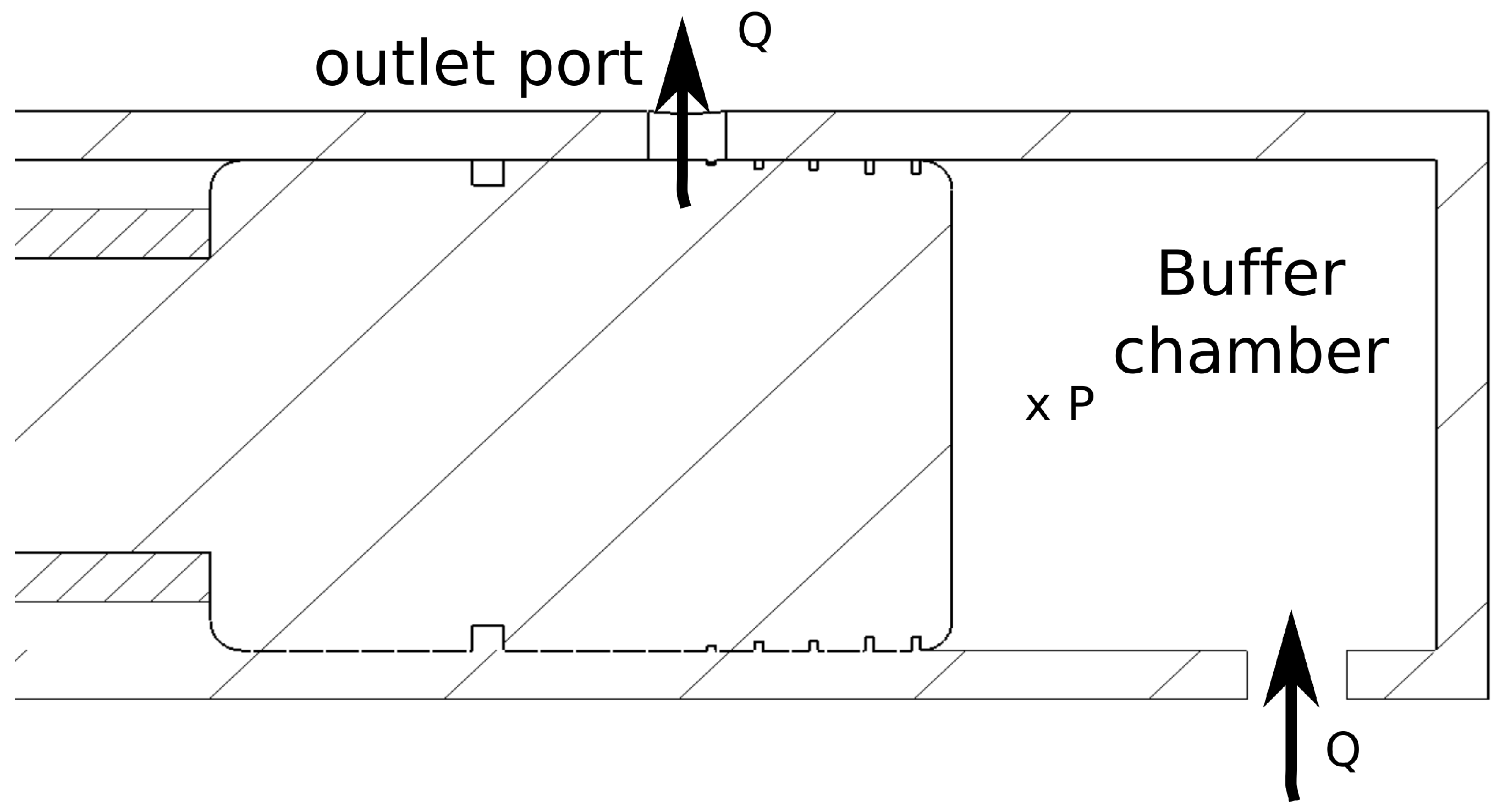
The numerical results have been compared and contrasted with the experimental measurements. A cylinder with a piston identical to the simulated geometries was exposed to a certain flow rate, and the pressure in the buffer chamber was measured. As in the numerical simulations, the piston was kept static, with a mechanical constraint, for the defined positions R12, R23, R34, R45 and R5. The flow rate was introduced in the buffer chamber through an additional inlet port, as schematically presented in Figure 5. For the centered piston experiments, the concentricity was imposed with two modified wear rings installed behind the seal. For the attached piston experiments, the wear rings were taken off and the piston was mechanically forced against the outlet port with a wedge.

The mechanical constraint of the piston in the experimental tests posed a question with respect to the velocity condition of the piston in the numerical experiments. In real acting pistons, and also in the present numerical simulations, this is essentially Poiseuille flow with some Couette component due to piston drag. Nevertheless, as the velocity ratio between the piston and the mean flow in the gap was the surface ratio between the piston and the gap surface, which, for our case, was around 80, the effect of the piston drag has been neglected. A rough estimation of the pressure-drop variation due to the velocity in the piston gave around 0.5%.

The pressure and flow rate were acquired with a Parker Service Master Easy, equipped with a pressure transducer PD-1500 and a hydraulic flow meter SCFT-0116-PD. The pressure transducer, installed in the buffer chamber and in the outlet port, had a measurement range of between 0 and 400 bar and an accuracy of 0.5% full scale, that is, 2 bar. The measurement range of the flow meter was between 4 and 60 L/min with an accuracy of 1% full scale, that is, 0.6 L/min. The temperature of the experiments was set at $60{}^{\circ }$C. The oil was class 32S, with a viscosity of $1.5\times {10}^{-5}{\mathrm{m}}^2/\mathrm{s}$ and a density of $921\mathrm{kg}/{\mathrm{m}}^3$ at this temperature. The temperature was monitored with the temperature sensor for the Parker Service Master Easy SCT-150-04-02. This sensor measured the temperature in the hydraulic flow meter, which was located just behind the outlet port of the cylinder. The temperature of the oil was controlled with a heat exchanger in an auxiliary circuit. Therefore, it could be assumed that the variation in the temperature of the oil flowing through the grooves was negligible. Additionally, it should be noted that the experimental rig was disassembled and reassembled, and the repeatability of experimental measurements had not been tested. Similarly, as a result of roundness uncertainty, experimental measurements can be affected by a particular orientation of the piston inside the cylinder. These issues have not been considered in the present work.

4. Results

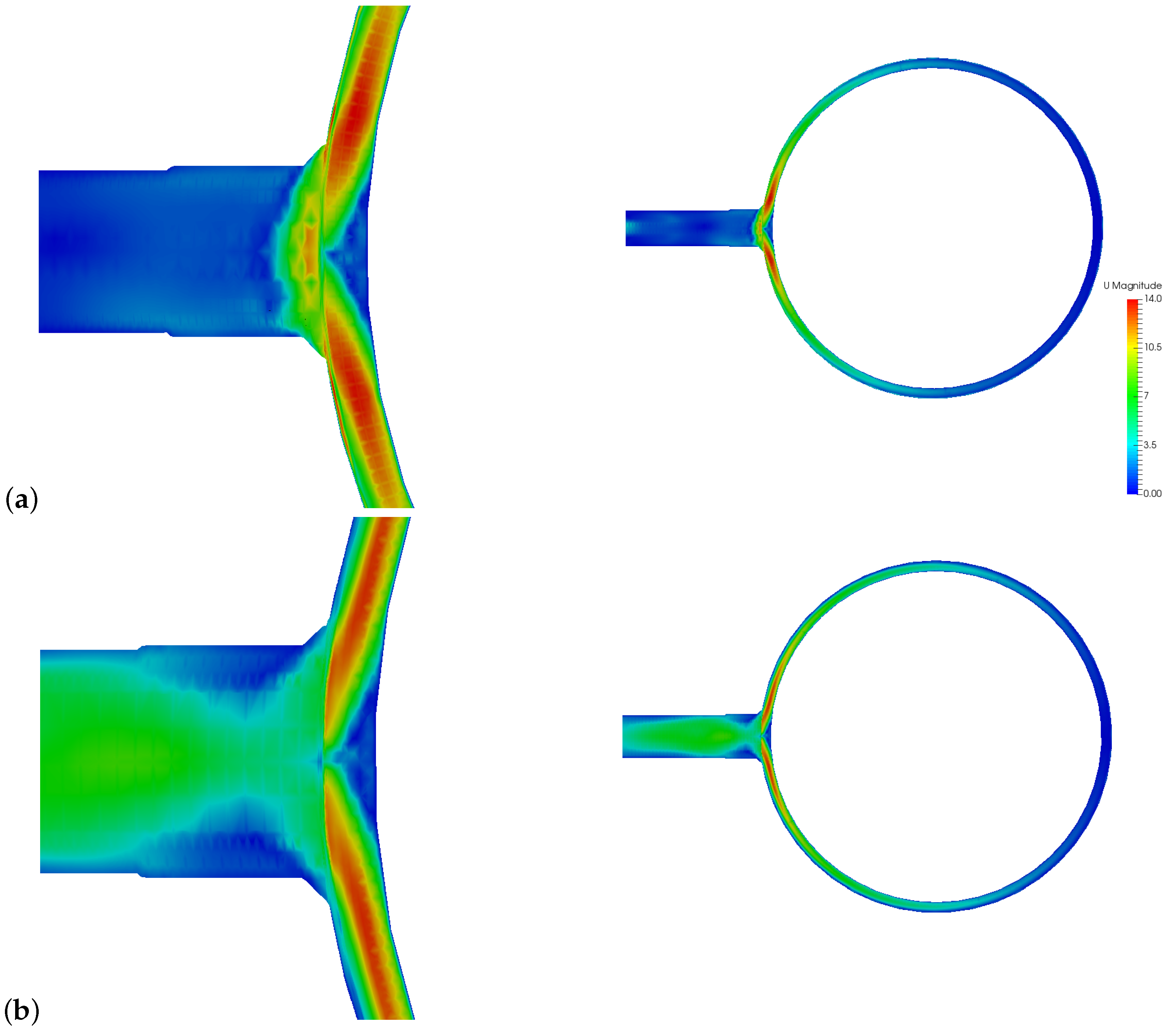
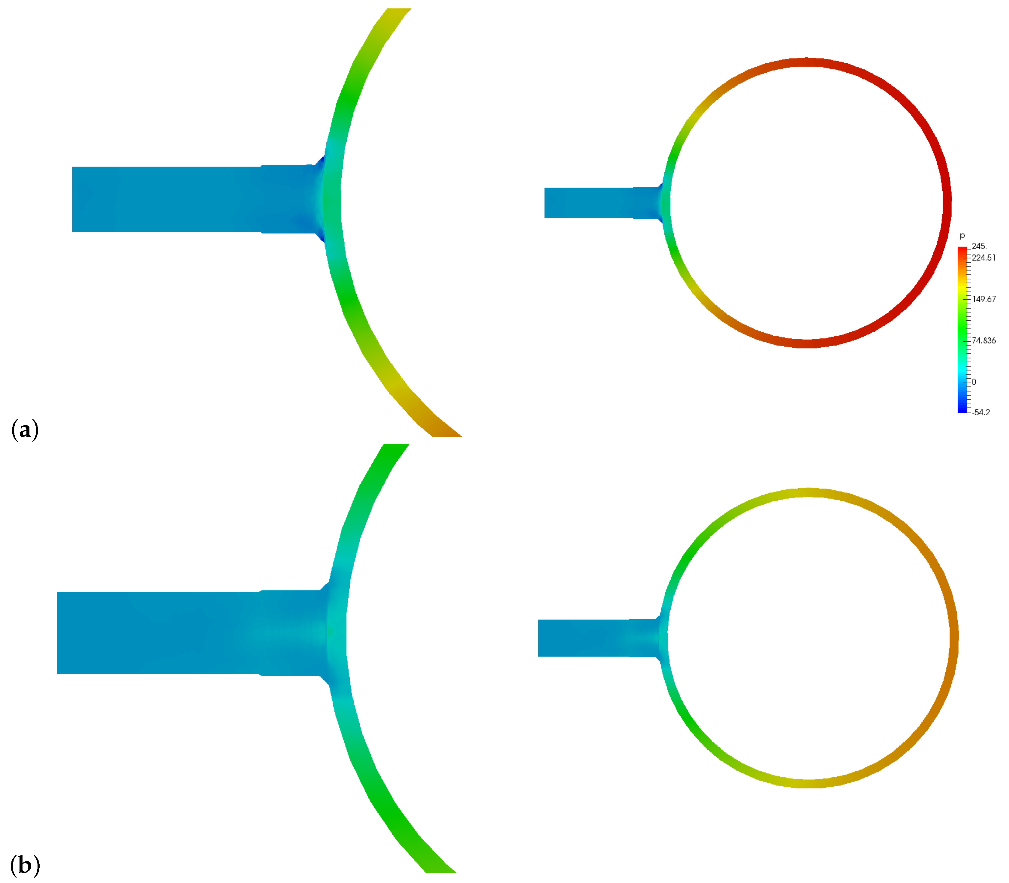
The distribution of the pressure and velocity magnitude has been plotted for all the grooves in all the piston positions, that is, grooves 1 and 2 for R12, grooves 2 and 3 for R23, grooves 3 and 4 for R34, grooves 4 and 5 for R45 and, finally, groove 5 for R5. These distributions have been extracted for the centered and off-centered piston. For the sake of illustration, the pressure and velocity contours are shown for the centered piston position R12 in Figure 6a,b and Figure 7a,b. These plots reveal that both the pressure and velocity magnitude take a constant value in almost half the circle, in the opposite side of the outlet port. 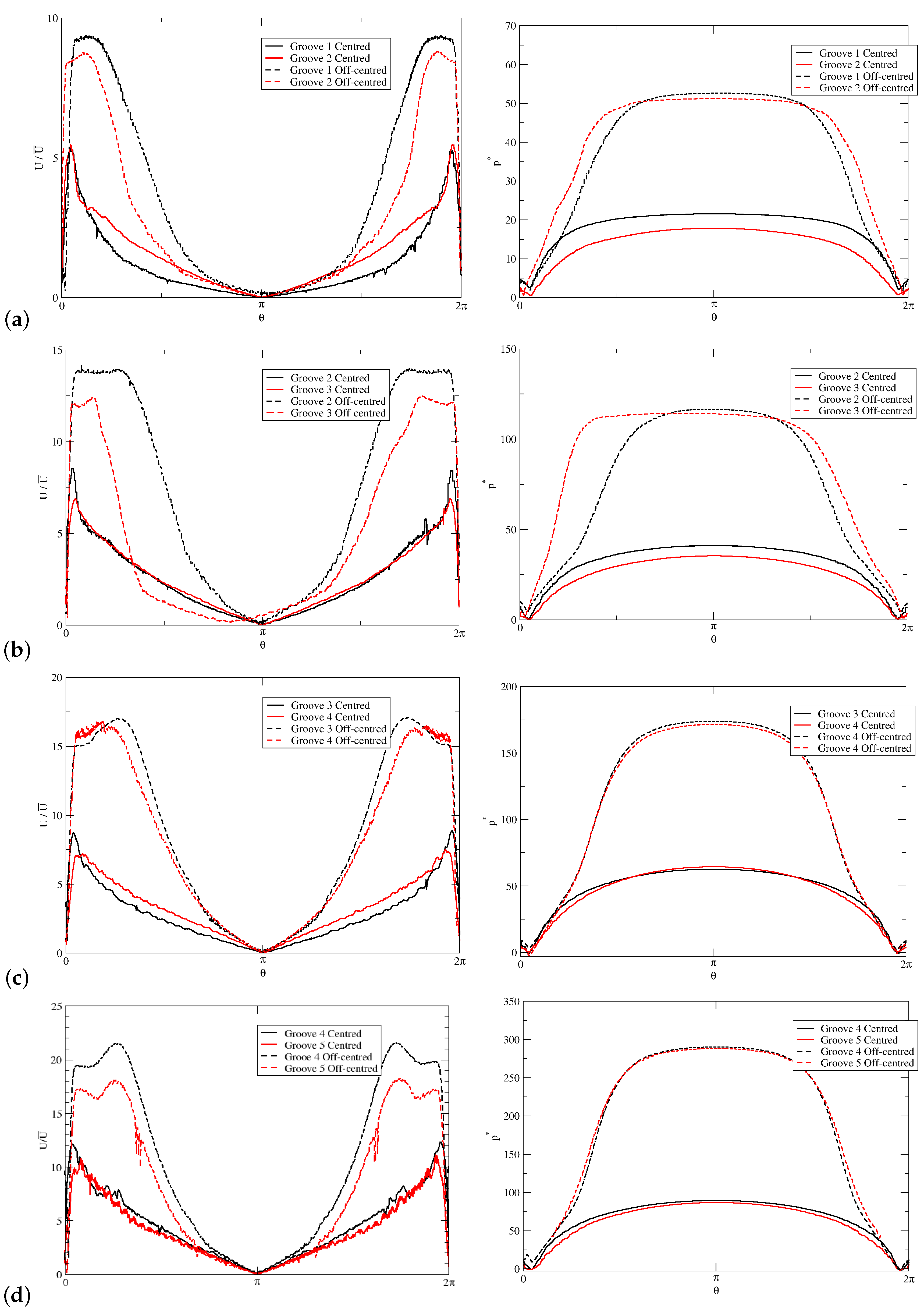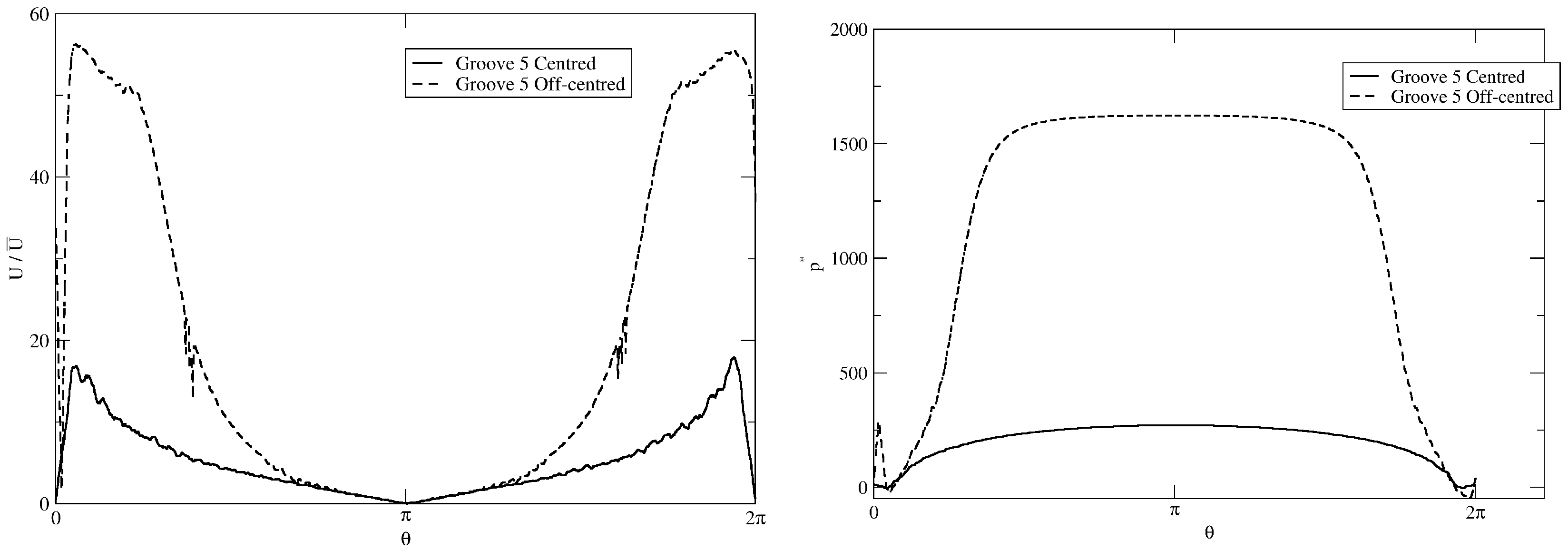Figure 8 and Figure 9 show the pressure and velocity distribution for all the grooves for the centered and off-centered piston in all the analyzed positions.

The velocity has been normalized with the average velocity in the outlet port, and the pressure has been normalized with the dynamic pressure in the outlet port. The graphs are plotted versus the polar angle, where 0 and $2\pi$ are the positions of the outlet port. The flow behaviour was clearly different for the centered and off-centered piston. Several points can be highlighted. First, the fluid velocity is much higher in grooves when the piston is radially displaced. When the piston is attached to the cylinder, all the flow is drawn through the grooves. When the piston is centered, this flow rate is distributed between the grooves and the gap between the cylinder and piston. 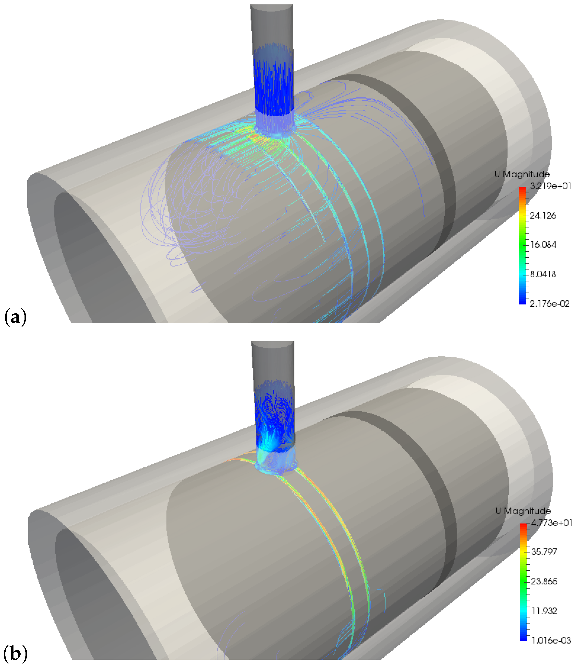Figure 10a,b shows the streamlines with the velocity for flow at position R34. Figure 10a shows the streamlines for the centered piston. It shows how fluid reaches the outlet port both through the grooves and the gap, particularly in the zone next to the outlet port. Part of the flow is even fed through grooves 2 and 5. Figure 10b shows streamlines for the attached piston. The fluid dynamic behaviour is completely different. The low is null in the gap, except in the opposite side of the outlet port, feeding only grooves 3 and 4 that lead fluid to the outlet port. Consequently the velocity is higher and so is the pressure drop. Second, the pressure is also much greater in grooves when the piston is attached to the cylinder. That indicates that, as expected, the pressure drop is larger through the grooves than in the gap. This pressure presents a central plateau that is more extended and flat for the attached piston.

Flow coefficients, defined as

$$C_D=\frac{Q}{S_o\sqrt{\frac{2\mathsf{\Delta }p}{\rho }}}$$

(6)

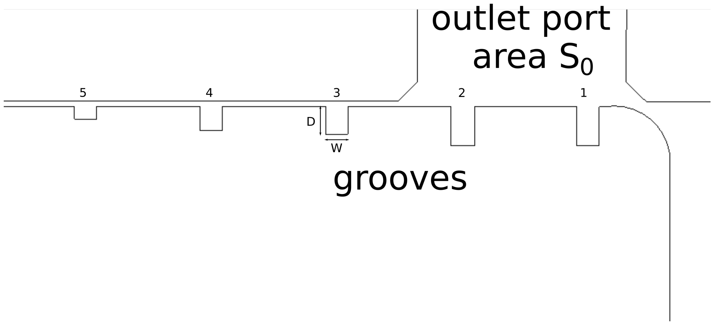
where Q is the flow rate; $S_o$ is the outlet port area, as depicted in Figure 2; $\mathsf{\Delta }p$ is the difference in pressure between the outlet port and buffer chamber in the cylinder; and $\rho$ is the density of the fluid, have been analyzed and compared with experimental measurements. The results are listed in

Table 2. Flow coefficients for numerical simulations and experimental measurements for centered piston.

Piston Position	CFD Results	Experimental Measurement	Experimental Reynolds	Deviation
R12	$0.104\pm 0.005$	$0.135\pm 0.026$	166	$-23.0$%
R23	$0.068\pm 0.003$	$0.055\pm 0.010$	161	+23.6%
R34	$0.050\pm 0.003$	$0.052\pm 0.010$	154	$-3.8$%
R45	$0.044\pm 0.002$	$0.031\pm 0.006$	92	+41.9%
R5	$0.026\pm 0.001$	$0.011\pm 0.001$	36	+136.4%

and

Table 3. Flow coefficients for numerical simulations and experimental measurements for off-centered piston.

Piston Position	CFD Results	Experimental Measurement	Experimental Reynolds	Deviation
R12	$0.068\pm 0.003$	$0.081\pm 0.003$	166	$-16.0$%
R23	$0.045\pm 0.002$	$0.047\pm 0.001$	142	$-4.2$%
R34	$0.036\pm 0.002$	$0.038\pm 0.001$	112	$-5.3$%
R45	$0.034\pm 0.002$	$0.025\pm 0.001$	75	+34.8%
R5	$0.012\pm 0.001$	$0.008\pm 0.001$	26	+50.0%

. Additionally, Reynolds numbers, as defined in Equation (3), are presented for experimental measurements. For all the numerical results, Reynolds number is 167. The error for the CFD results has been estimated from uncertainty due to mesh convergence. As this gives an uncertainty of 9% for the pressure drop, this leads to an estimated error of 5% for $C_D$.

The Reynolds number was kept constant in the CFD simulations for the sake of simplicity. In the case of the experimental measurements, the value of the flow rate and, consequently, of the Reynolds number was limited by the capacity of the pressure transducer. Because pressure loss was appreciably higher for positions R45 and R5, the flow rate had to be reduced in order to adequately measure the pressure in the buffer chamber.

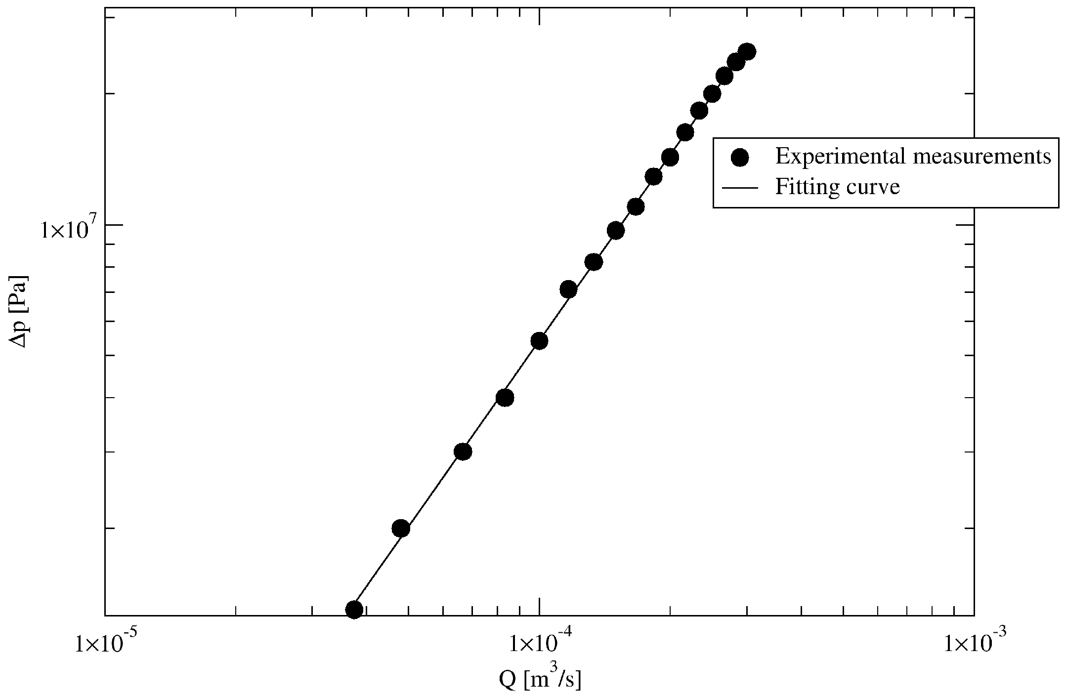
As a consequence of the increase in the pressure loss, the values of the flow coefficients decreased with the position of the piston. Nevertheless, a significant discrepancy between the CFD calculation and experimental measurements was found, essentially as a result of the difference in the Reynolds numbers. In order to correct the numerical calculation, a correlation between the pressure drop and flow rate was estimated from experimental tests. These results, presented in Figure 11, suggest that the pressure drop scales with the flow rate as

$$\mathsf{\Delta }p\sim Q^{1.4}$$

(7)

Using this correlation with Equation (6), this yields

$$C_D\sim {\mathrm{Re}}^{0.3}$$

(8)

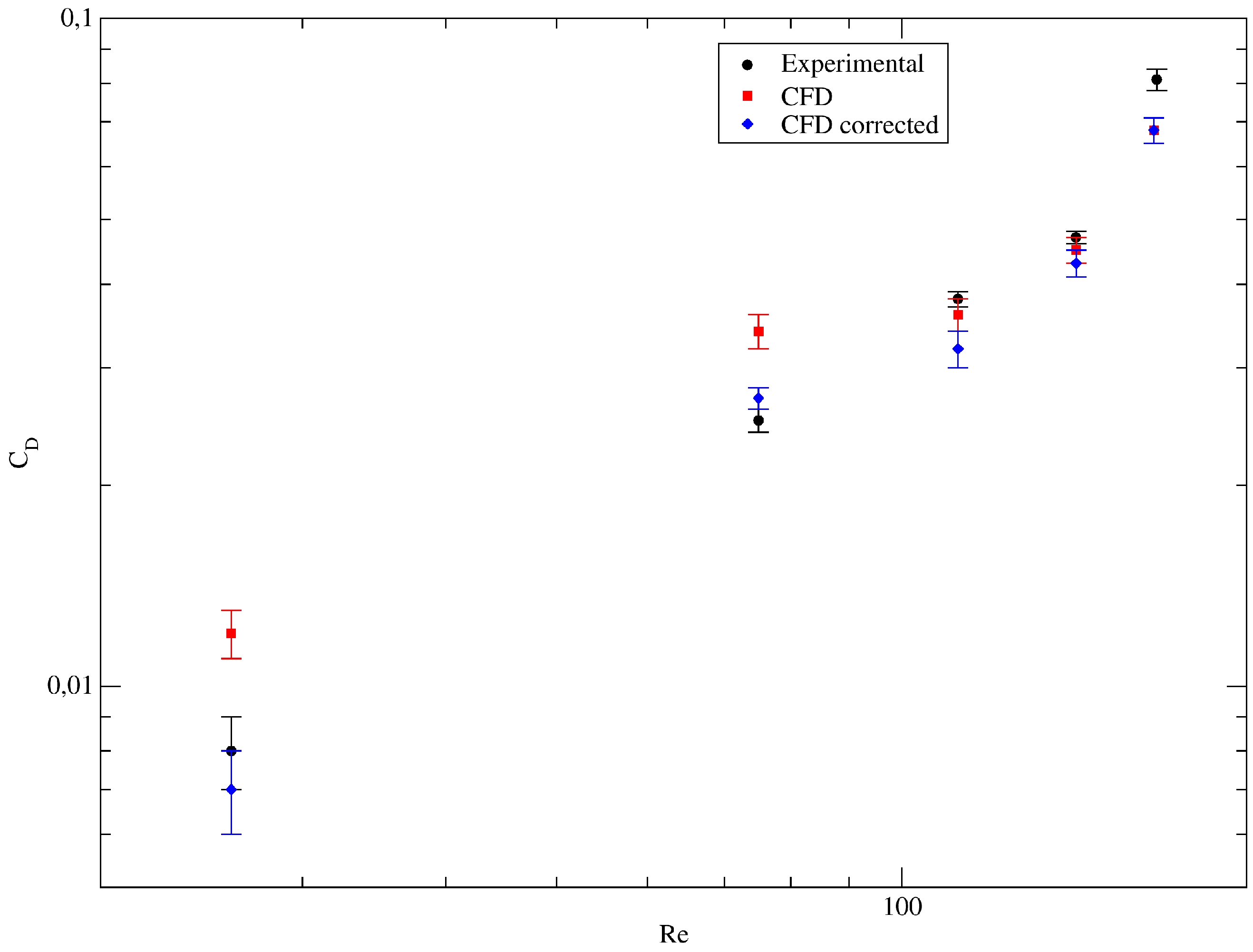
This correlation can be used to correct the numerical flow-rate coefficients. The corrected results are listed in

Table 4. Flow coefficients for numerical simulations and experimental measurements for off-centered piston.

Piston Position	Corrected CFD Results	Experimental Measurement	Experimental Reynolds	Deviation
R12	$0.068\pm 0.003$	$0.081\pm 0.003$	166	$-16.0$%
R23	$0.043\pm 0.002$	$0.047\pm 0.001$	142	$-8.5$%
R34	$0.032\pm 0.002$	$0.038\pm 0.001$	112	$-15.8$%
R45	$0.027\pm 0.001$	$0.025\pm 0.001$	75	+8.0%
R5	$0.007\pm 0.001$	$0.008\pm 0.001$	26	+1.25%

and are also plotted, along with the non-corrected $C_D$, in Figure 12. The deviation for R23 and R34 has been increased, but now the agreement is very good between R45 and R5, for a lower Reynolds number. In general, the deviation from experimental measurements was bounded, with a maximum underestimation of 16%. This deviation was considered acceptable, given that the error in the measured gap height, due to roundness uncertainty in the cylinder and piston, was around 6%; hence, this led to an error of around 10% in the numerical $C_D$ estimation.

5. Discussion and Conclusions

Numerical CFD simulations were conducted for the analysis of the pressure drop in a groove-machined piston for the cushioning system of a hydraulic cylinder. The aim of the work is to provide a method to estimate the values for a certain design of a piston groove pattern. This method has been used in a dynamical system simulation that is able to predict the behaviour of the cushioning performance of the cylinder.

The numerical results, obtained with a constant value of Re = 167 have been compared with experimental measurements. The value of the numerical Reynolds number was constant, because the estimated value of the flow-rate coefficient had to be used in the dynamic simulation with an a priori unknown Reynolds number. The proposed method is to numerically estimate a $C_D$ value with a given Re and then to correct it for a certain velocity condition in the cushioning process. The experimental Reynolds number was bounded by the limitation of the pressure transducer used. The agreement was acceptable for similar Reynolds numbers, in positions R23 and R34 for the attached piston, considering that, according to the definition of the flow-rate coefficient (Equation (6)) and the confidence level estimated in the grid independence analysis, the uncertainty in the values of $C_D$ was about 5%. For the centered piston, the agreement was only good for R34. For R12, both the attached- and centered-piston simulation underestimate the value of the flow coefficient, at 23% and 16%. The reason for this disagreement was likely the more complex flow in the rounded corner, which led the flow towards the outlet port (see Figure 2 for position R12 of piston). As a future work for the improvement of the method, a better mesh that could resolve the boundary layer and the flow separation in this zone could likely allow for a better estimation of $C_D$ for position R12. For positions R45 and R5, with low Reynolds numbers, the value of $C_D$ was highly overestimated, due to the difference in the Reynolds number. These estimations of $C_D$ can be corrected if the correlation between the pressure drop and flow rate is known. This correlation was experimentally obtained for a range of the Reynolds number between 12 and 92 for position R45 with the piston attached to the cylinder, yielding the expression of Equation (8) that allows for correcting $C_D$ with the Reynolds number. This correction gives an excellent agreement for R45 and R5 while it worsens the agreement between R23 and R34. Nevertheless, the overall results are better than the uncorrected estimations. This method for the pressure-drop coefficient estimation can contribute to the development of a dynamic system simulation and to the proposing of an enhanced design method for a cylinder cushioning system.

References

1. Majumdar, S.R. Oil Hydraulic Systems: Principles and Maintenance; Tata McGraw-Hill: New York, NY, USA, 2001; p. 548. [Google Scholar]
2. Koshinen, K.T.; Vilenious, M.; Tikka, K. On the damping of a hydraulic cylinder drive. In Proceedings of the Sixth Scandinavian International Conference on Fluid Power, Tampere, Finland, 26–28 May 1999; Tampere University of Technology: Tampere, Finland, 1999; pp. 499–518. [Google Scholar]
3. Das, J.; Mishra, S.K.; Saha, R.; Mookherjee, S.; Sanyal, D. Actuation dynamic modeling and characterization of an electrohydraulic system. Proc. Inst. Mech. Eng. Part I 2016, 230, 537–550. [Google Scholar] [CrossRef]
4. Borghi, M.; Milani, M.; Conrad, F. Mechanical Cushion Design Influence on Cylinder Dynamics; SAE International: Warrendale, PA, USA, 2005. [Google Scholar]
5. Schwartz, C.; De Negri, V.J.; Climaco, J.V. Modeling and analysis of an auto-adjustable stroke end cushioning device for hydraulic cylinders. J. Braz. Soc. Mech. Sci. Eng. 2005, 27, 415–425. [Google Scholar] [CrossRef]
6. Prahallad, C.; Raveender, A. Modeling and Optimization of Cushioning System in Hydraulic Cylinder to achieve Performance Characteristics. Imp. J. Interdiscip. Res. 2017, 3, 2122–2128. [Google Scholar]
7. Gao, Q.; Wang, X.; Rong, M.; Fu, Y.; Li, X. Optimization design on step-shape cushioning for hydraulic operating mechanism of high voltage circuit breakers. In Proceedings of the 2016 International Conference on Condition Monitoring and Diagnosis (CMD), Xián, China, 25–28 September 2016; pp. 226–229. [Google Scholar]
8. Kenyon, K.E. Flow past a Groove. Nat. Sci. 2015, 7, 100–102. [Google Scholar] [CrossRef]
9. Mezghania, S.; Demircia, I.; Zahouanib, H.; El Mansoria, M. The effect of groove texture patterns on piston-ring pack friction. Precis. Eng. 2012, 36, 210–217. [Google Scholar] [CrossRef] [Green Version]
10. Zawistowski, T.; Kleiber, M. Gap Flow Simulation Methods in High Pressure Variable Displacement Axial Piston Pumps. Arch. Comput. Methods Eng. 2017, 24, 519–542. [Google Scholar] [CrossRef]
11. Bergada, J.M.; Watton, J.; Haynes, J.M.; Davies, D.L. The hydrostatic/hydrodynamic behaviour of an axial piston pump slipper with multiple lands. Meccanica 2010, 45, 585–602. [Google Scholar] [CrossRef] [Green Version]
12. Bergada, J.M.; Kumar, S.; Davies, D.L.; Watton, J. A complete analysis of axial piston pump leakage and output flow ripples. Appl. Math. Model. 2012, 36, 1731–1751. [Google Scholar] [CrossRef]
13. Hao, M.; Qi, X.Y. Modeling Analysis and Simulation of Hydraulic Axial Piston Pump. Adv. Mater. Res. 2012, 430–432, 1532–1535. [Google Scholar] [CrossRef]
14. Ivantysynova, M.; Huang, C. Investigation of gap flow in displacement machines considering eslastohydrodynamic effect. Proc. JFPS Int. Symp. Fluid Power 2002, 2002, 219–229. [Google Scholar] [CrossRef]
15. Kumar, S.; Bergada, J.M. The effect of piston grooves performance in an axial piston pumps via CFD analysis. Int. J. Mech. Sci. 2012, 66, 168–179. [Google Scholar] [CrossRef]
16. Algar, A.; Codina, E.; Freire, J. Experimental Study of 3D Movement in Cushioning of Hydraulic Cylinder. Energies 2017, 10, 746. [Google Scholar] [CrossRef]
17. Šidlof, P. Numerical simulation of deformation of dynamic mesh in the human vocal tract model 2 Approaches for calculation of the mesh deformation in OpenFOAM. EPJ Web Conf. 2015, 6, 5–8. [Google Scholar]
18. Roache, P.J. Verification and Validation in Computational Science And Engineering; Hermosa Publishers: Albuquerque, NM, USA, 1998; p. 446. [Google Scholar]
19. Ferizigner, J.H.; Peric, M. Computational Methods for Fluid Dynamics, 3rd ed.; Springer: Berlin, Germany, 2002. [Google Scholar]
20. Menter, F.R. Improved Two-Equation k-ω Turbulence Models for Aerodynamic Flows; Technical Report; NASA Technical Memorandum: Moffet Field, CA, USA, 1992.
21. Casey, M.; Wintergerste, T. (Eds.) Best Practice Guidelines; ERCOFTAC: Brussels, Belgium, 2000. [Google Scholar]
22. Wilcox, D.C. Turbulence Modeling for CFD; DCW Industries: La Cañada Flintridge, CA, USA, 2006; p. 522. [Google Scholar]
23. Russo, F.; Basse, N.T. Scaling of turbulence intensity for low-speed flow in smooth pipes. Flow Meas. Instrum. 2016, 52, 101–114. [Google Scholar] [CrossRef]
Figure 1. 3D view of cylinder, with the outlet port, and the piston with five grooves, in position R12.
Energies 10 01704 g001
Figure 2. Scheme of grooves in piston with the position R12. First and second grooves are facing outlet.
Energies 10 01704 g002
Figure 3. Structured background mesh for cylinder and piston meshing. Detail of gap meshing with five layers is also shown.
Energies 10 01704 g003
Figure 4. Mesh for gap between piston and cylinder, and outlet pipe.
Energies 10 01704 g004
Figure 5. Schemes for experimental set-up of flow rate through buffer chamber in cylinder. The shown position is R5.
Energies 10 01704 g005
Figure 6. Velocity magnitude distribution for grooves 1 (a) and 2 (b) for position R12 with detail of junction with outlet port. Units of velocity are m/s.
Energies 10 01704 g006
Figure 7. Specific pressure distribution for grooves 1 (a) and 2 (b) for position R12 with detail of junction with outlet port. Units of specific pressure are J/kg.
Energies 10 01704 g007
Figure 8. Dimensionless velocity distribution and dimensionless pressure distribution for groove positions R12 (a), R23 (b), R34 (c) and R45 (d). Continuous lines are for centered piston and dashed lines are for off-centered pistons.
Energies 10 01704 g008
Figure 9. Dimensionless velocity distribution and dimensionless pressure distribution for groove 5 in position R5. Continuous lines are for centered piston and dashed lines are for off-centered pistons.
Energies 10 01704 g009
Figure 10. Streamlines for outlet flow for position R34 for centered piston (a) and attached piston (b).
Energies 10 01704 g010
Figure 11. Correlation between pressure drop and flow rate for piston position R45. Reynolds number ranges from 12 to 92.
Energies 10 01704 g011
Figure 12. Flow-rate coefficients versus Reynolds number for experimental measurements, CFD computations and corrected CFD results, using correlation Equation (8).
Energies 10 01704 g012