A Computed River Flow-Based Turbine Controller on a Programmable Logic Controller for Run-Off River Hydroelectric Systems

1
College of Engineering, Universiti Tenaga Nasional (UNITEN), Jalan Ikram-Uniten, Kajang 43000, Selangor, Malaysia
2
Generation Research Department, Tenaga Nasional Berhad Research (TNBR), Kajang 43000, Selangor, Malaysia
*
Author to whom correspondence should be addressed.
Energies 2017, 10(11), 1717; https://doi.org/10.3390/en10111717
Submission received: 31 July 2017
/
Revised: 15 September 2017
/
Accepted: 18 September 2017
/
Published: 27 October 2017
(This article belongs to the Special Issue Hydropower 2017)
Abstract
:The main feature of a run-off river hydroelectric system is a small size intake pond that overspills when river flow is more than turbines’ intake. As river flow fluctuates, a large proportion of the potential energy is wasted due to the spillages which can occur when turbines are operated manually. Manual operation is often adopted due to unreliability of water level-based controllers at many remote and unmanned run-off river hydropower plants. In order to overcome these issues, this paper proposes a novel method by developing a controller that derives turbine output set points from computed mass flow rate of rivers that feed the hydroelectric system. The computed flow is derived by summation of pond volume difference with numerical integration of both turbine discharge flows and spillages. This approach of estimating river flow allows the use of existing sensors rather than requiring the installation of new ones. All computations, including the numerical integration, have been realized as ladder logics on a programmable logic controller. The implemented controller manages the dynamic changes in the flow rate of the river better than the old point-level based controller, with the aid of a newly installed water level sensor. The computed mass flow rate of the river also allows the controller to straightforwardly determine the number of turbines to be in service with considerations of turbine efficiencies and auxiliary power conservation.
1. Introduction
Energy generated from renewable sources has grown tremendously in the past few decades in the first world countries on the European and North American continents. This growth has been stimulated by directives, incentives, regulations and technology advancements, whereas in Malaysia, government bodies such as the energy commission have introduced feed in tariffs to increase the penetration of photovoltaic energy in the country, while private companies such as Tenaga National Berhad (TNB), the biggest utility company in Malaysia, have embarked on many renewable energy projects, mostly focused on solar photovoltaic, for remote residential customers, and recently on large commercial solar farms.
Other initiatives by TNB include efforts to improve the efficiency of some existing hydroelectric plants in Malaysia, mostly targeting operational improvements. As an example a gain in the operational efficiency of hydropower plants can be accomplished by improving reservoir management to reduce spillages and also by maintaining larger hydraulic heads behind dams. Beside major hydroelectric plants in the Malaysia Peninsula, TNB also owns and operates several small hydroelectric systems, including a run off river one located in the state of Perak.
This paper is a case study for a run-off river hydroelectric operation optimization with a proposed computed river flow-based controller to improve energy production. The location of the studied hydroelectric system is in the state of Perak, in the northern part of the Malaysia Peninsula. In addition to hydroelectric power generation, river flows are also useful for other purposes, therefore some samples of contemporary data collections for rivers found in the literature are included and briefly described.
1.1. Hydroelectric Operational Optimization Case Study
The hydroelectric system for the case study is an unmanned and very remote cascaded run-off river hydropower unit, consisting of two power stations: an upper station (2 × 7.5 MWe) and a lower station (2 × 27 MWe), as illustrated in Figure 1.
The main source of water for this hydroelectric system comes from a river known as Piah which feeds the upper station. As for the lower station, it has a thirteen kilometer multi-inlet tunnel to deliver water discharged from the upper station and water diverted from small nearby tributaries. To produce a maximum power of 55 MWe, the lower station has two four-nozzle vertical Pelton turbines wherein each turbine is capable of driving a 27.5 MWe generator. A similar set-up had been applied to the upper station, which also equipped with two Pelton type turbines and two generators to produce a combined maximum power output of 15 MWe.
This run-off river hydropower system, constructed in the late 1980s, had a control system with point level type sensors or float switches. However this type of controller was often prone to “control hunting”, a phenomenon had been happened since the early days of this power station. Due to this control hunting issue, the practice adopted at this hydroelectric was manual operation of the turbines. The manual operation was setting the turbine outputs to fixed values lower than the river flow, allowing spillages higher than the design value as safe conservative procedures. The spill flow for the lower station’s intake pond is shown in Figure 2.
To improve energy production, instead of simply replacing the old point level based controller, a new type of controller has been installed at the lower station. Unlike the old controller, the new controller uses computed river mass flow rate rather than merely depending on water level alone to regulate the turbine output set points. Rather than having to install expensive flow meters with high installation and maintenance costs, the mass flow rate of the river has been computed by control volume analysis and by considering the conservation of mass at the intake pond. The controller with its associated computations has been realized on a programmable logic controller (PLC).
The incoming river mass flow rate can be computed if the pond volume rate of change and pond exit flows are known. The pond volume rate of change can be calculated from its geometric shape and water level variation. The pond exit flows are made up of spillages and turbine discharges. As for the turbine discharge flows, one can use the existing generator power meters to derive them, while spill flow corresponds to height of water above the dam crest.
1.2. Related River Flow Measurement Works
In addition to hydroelectric regulations, river flow data are also useful for many other purposes. For example Marsh examined initiatives in the United Kingdom aimed at addressing contemporary data needs and maximizing strategic utilization of national archived river flow data. Changes in climate pattern, land cover and water utilization, together with changing legislation will increase demand for river data [1]. Cretin et al. proposed an image-based method for discharge measurements for river gauging in an experiment on the Iowa River, at Iowa City, IA, USA. Video recording images and particle image velocimetry (PIV) were used to estimate surface velocities for the imaged areas using naturally occurring foam as a flow tracer. The surface velocities were then estimated along the surveyed river section, and river discharge was computed using standard velocity-area methods over a selected cross section. This method has limitations such as the need for a recognizable tracer foam and survey information of the channel cross section, as well as problems associated with shadows and reflections on the water surfaces [2]. Muste et al. [3] suggested large-scale particle image velocimetry (LSPIV) to measure normal flows and floods for river in Iowa, USA. Presently, a method known as acoustic Doppler current profiler (ADCP) measures water velocities in three dimensions. The velocities are then utilized as parameters to derive river flow [4]. Flow measurement comparisons between LSPIV with the ones obtained with ADCP have been studied by several research groups.
2. Run-Off River Hydroelectric Plants
Most large hydroelectric plants have turbine controllers that regulate turbine intake flow according to energy demands, while storing the extra inflow of water from feeding rivers in its reservoir. Beside energy generation and flood mitigation, a river with a power generation reservoir needs to regulate the downstream flow for farming water supplies, drinking water as well as release of minimum riparian flow for the life of the river itself [5,6].
Unlike large hydroelectric plants, a run-off river power plant has a small size reservoir that cannot store potential energy except for holding small amounts of water, sufficient to avoid the penstock’s pressure transients as turbines vary their outputs. As a run-off river scheme is designed not to store potential energy of water, except for small amounts, its operation strategy is to maximize turbine outputs according to the available river flow. Reducing spillage means more water goes into turbines, and this improves its overall annual generation output. This consequently lowers the total carbon emissions of all the fossil-based power plants in the country.
At this run-off hydroelectric system, its Pelton turbines had been regulated by a controller which depends solely on the point type water level (float switches). Such a controller has limitations to perform regulation well when the water level is wrongly represented or incorrect. Examples of wrong water level representations include high water level readings though the actual water levels at the dam are normal or when river flows are regular. These phenomena can occur when the dam’s trash rack is blocked, which causes water level sensors upstream of the rack to read high levels though in fact the penstock has an insufficient volume of water. In this case the controller commands turbines to increase their output assuming a high river flow, though the penstock is actually deprived of water, as water flow is blocked from going into turbine inlets by the choked trash racks.
Other drawbacks include level sensors that may detect low intake water levels when there is a transient of low pressure regimes created in the penstock power tunnel due to fast opening of turbine control valves, though the actual water levels or river flows are normal. In addition, this type of controller is sensitive, and reacts hastily as water level fluctuations within a short of duration when disturbances occurs. Such fast response does not suit with the type of hydroelectric system that has a relatively small intake pond size compared to the much larger power tunnel volume, for example, and intake pond volume of 5000 m3 compared to 50,000 m3 of the power tunnel.
Due to the described drawbacks with unmanned operations, this run-off river station had been run manually, allowing much higher spillage than the riparian flow. Several approaches could be employed to improve the turbine control system at the hydroelectric station. One possible approach was to replace the existing water level-based controller with a similar one but with improvements. The approach selected for this project however has been a new type of controller that determined set points of turbine intakes according to the mass flow rate of the river. In order to avoid installing new expensive equipment, a computed river flow has been proposed instead. The implemented controller has been capable of regulating turbine outputs according to the fluctuation of river flows. Consequently spillage has been reduced, resulting in better annualized energy outputs.
3. River Flow Computations
As mentioned in the Section 2, as an alternative to replacing the old control system with the latest water level based turbine controller, a new controller that is able to calculate turbine operating set points based on river flow has been adopted instead. Therefore to measure river flow, the option is either to install flow measurement sensors or devising indirect methods of estimating flow. However, measurements of flows of multiple rivers that fed the intake ponds often have challenges due to remote locations and a lack of power supply, especially for run-off river hydropower units. The following subsections describe different methods for measuring flow of the river.
3.1. River Flow Measurement Basics
The determination of a river flow rate (usually symbolized as Q) requires two measurements: wetted area (A, in m2) of the cross section of a river and mean velocity of the moving water (V, in m/s) [6,7]. The product of these two measurements is flow (Q, m3/s) in volume rate per unit time or flow:
The wetted area is a function of the water level and cross section geometry, while mean velocity is the average speed distribution across a river channel from the surface to the bottom as well as from the sides to the center of the river, to accommodate friction and cross-section irregularities. The flow of the river is usually highest at the surface and center of the river. The velocity can be measured by rotor or vane type instruments. These instruments are typically found in early generations of hydroelectric systems, with newer devices such as ADCPs are becoming popular. However, ADCP is relatively expensive compared to water level sensors that often used for river gauging. Water level had often being measured by submersible hydrostatic sensors in many early power station projects. Also, some instruments have floats with switches as primary water level measurements to regulate hydro-turbines at some hydroelectric sites. Most of these kinds of hydrostatic sensors needed constant corrective maintenance since they are exposed to mud present in the water. Therefore maintenance personnel often has to go into the water to clean and calibrate them. Presently, non-contactable water level sensor types such as ultrasound, radar or laser sensors are common, while numerous existing small hydroelectric plants are considering these sensors type for better level measurements options.
3.2. Proposed River Flow Estimation
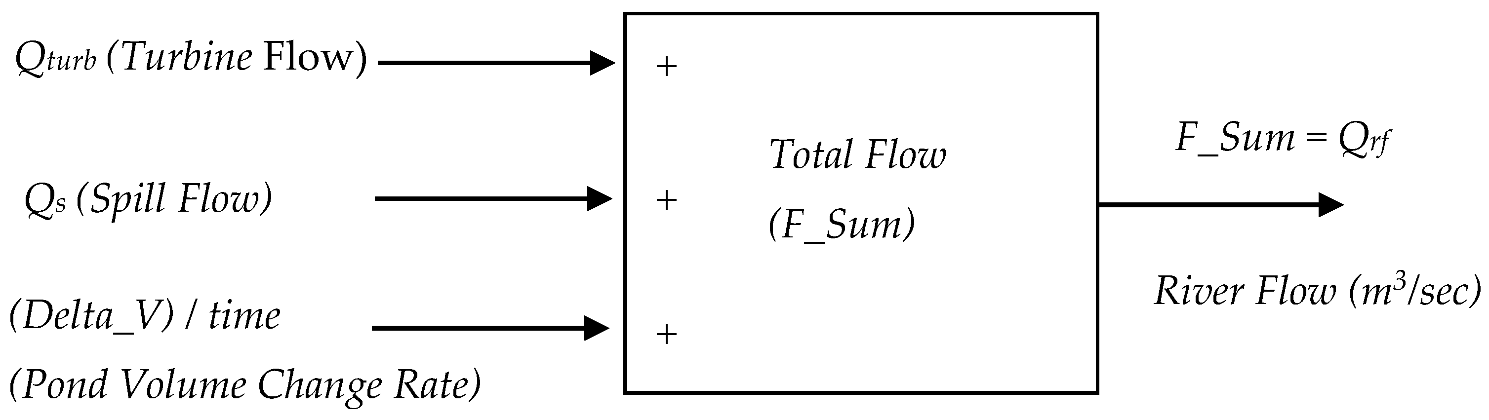
Instead of procuring expensive non-contactable type flow meters to measure the river flow, a new simple computing technique to estimate river flow is proposed. River flow can be computed by summing total turbine discharge flows, rate change of reservoir volumes and spillages. Let’s say the average river flow that feeds the lower station’s intake pond is Qrf. Using mass conservation, therefore the river flow should equal the summation of spillage (Qs), intake pond volume change (Delta_V/time) and discharge flows of turbines (Qturb), as given in either Equation (2) or (3). The summation is further illustrated in Figure 3 as a preliminary step prior to going into details of reasons that numerical integration is required to derive the river flow:
Also, the turbine flow Qturb (in both Equations (2) and (3)) should be the combination flows from all turbines that are in operation. Equation (2) or (3) demands multiple flow measurements or methods to calculate flow, as well a method to obtain intake pond volume change rates.
Referring to Figure 3, it is not possible to measure the intake pond volume rate directly in order to obtain the river flow (Qrf). Instead the volume rate has to be computed using pond levels (water level sensor) measured at different times. Therefore a water level sensor needs to be installed to measure the water levels at the intake pond if the existing one is defective or does not possess appropriate resolution and accuracy; in our case a robust radar type sensor had been installed.
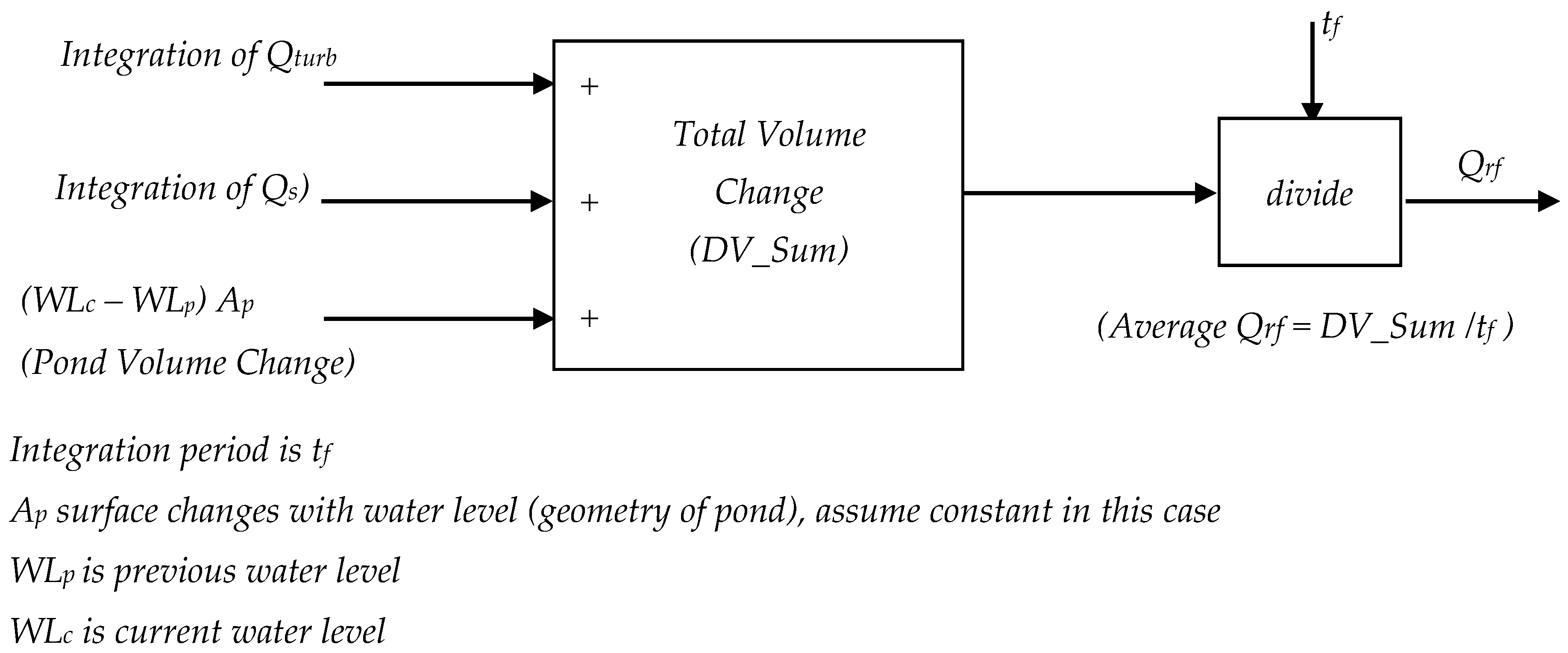
Integrating Equation (3) over time, we obtain Equation (4) which provides us with the information of fluid mass entering and exiting the system within time tf. Therefore, Figure 3 becomes Figure 4 where an integration method is required since pond volume change rate cannot be measured directly. Also to eliminate noises and mitigate errors, multiple samplings of water level measurements are needed.
From Figure 4, the average river flow (Qrf) for a time interval (tf) becomes Equation (4):
where = spillage (m3/s); = turbine discharge (m3/s) for both turbines; = previous dam water level (mSLE is meter sea level elevation); = current dam water level (mSLE) after = average water surface area for intake pond (m2); = final time for control regulation interval (s); also = integration period.
As WLc and WLp are readings that originate from the same water level sensor, measurement times should be appropriately apart with multiple samples taken to reduce measurement errors. Also, as turbine discharge flow and spillages fluctuate over time, therefore their summation to derive river flow necessitates integration methods.
As illustrated in Figure 4, the intake pond volume changes (either the increment or decrement rate) is the product of pond water surface average area by the water height difference over a selected time interval T as in Equation (5). T is equals to integration period. The height difference of water level is obtained by deducting the previous water level (WLp) from the current water level (WLc). Both water levels are readings from the same water level sensor with appropriate measurement times apart (WLp and WLc are measured at start and end of integration period, respectively). The pond surface area differs at different water levels, however as water variation within our case was less than 0.75 m, its average of 9000 m2 was used for simplification:
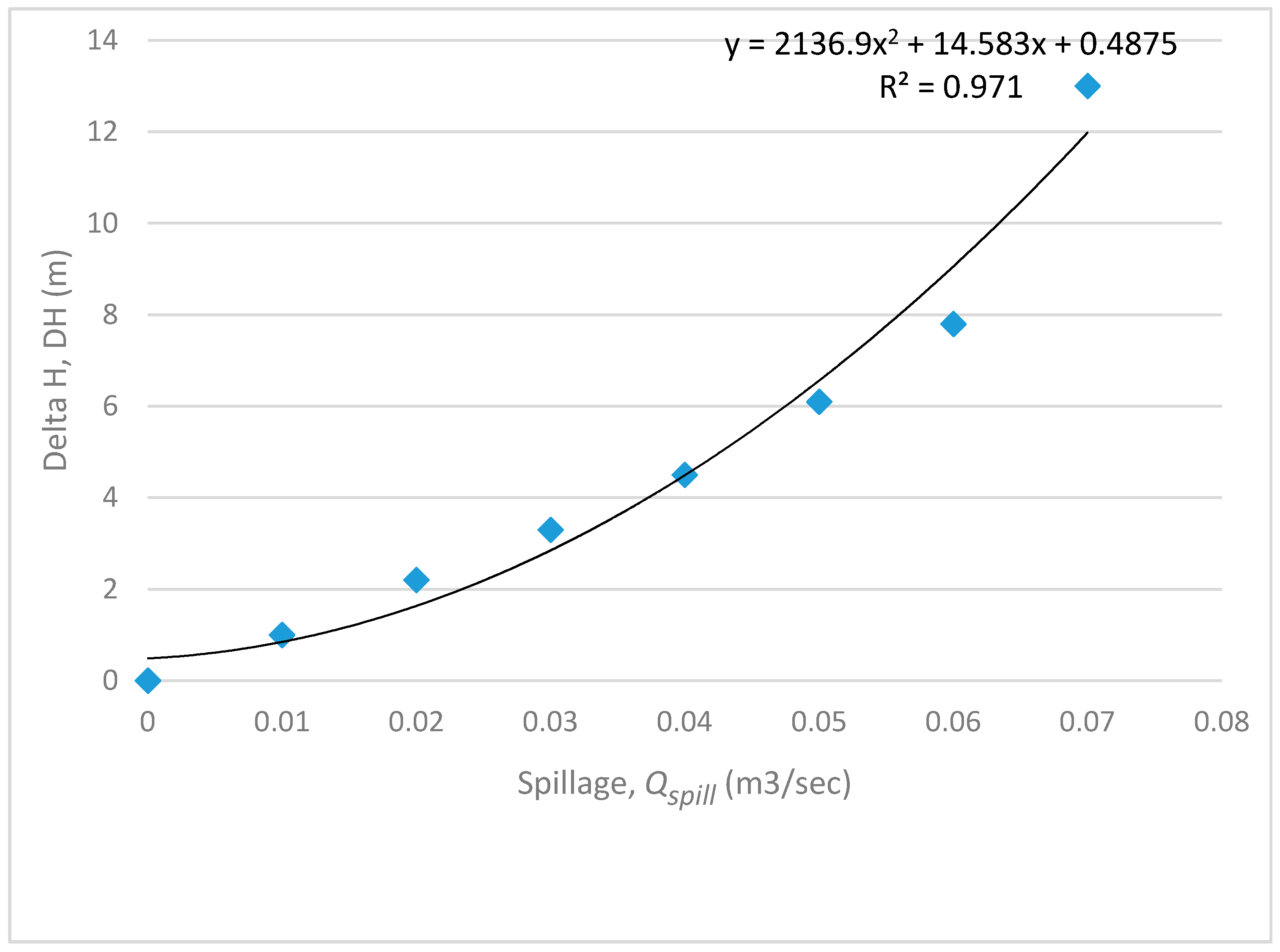
As for the spill flow, its relation with water level above dam crest is tabulated in Table 1. Spillage flow is Qs, while the height difference between water level and the dam crest is Delta_H or DH. Using values tabulated in Table 1 that had been obtained by measurements, using quadratic curve fitting, yielding Equation (6). The plot of spillage versus DH is shown in Figure 5:
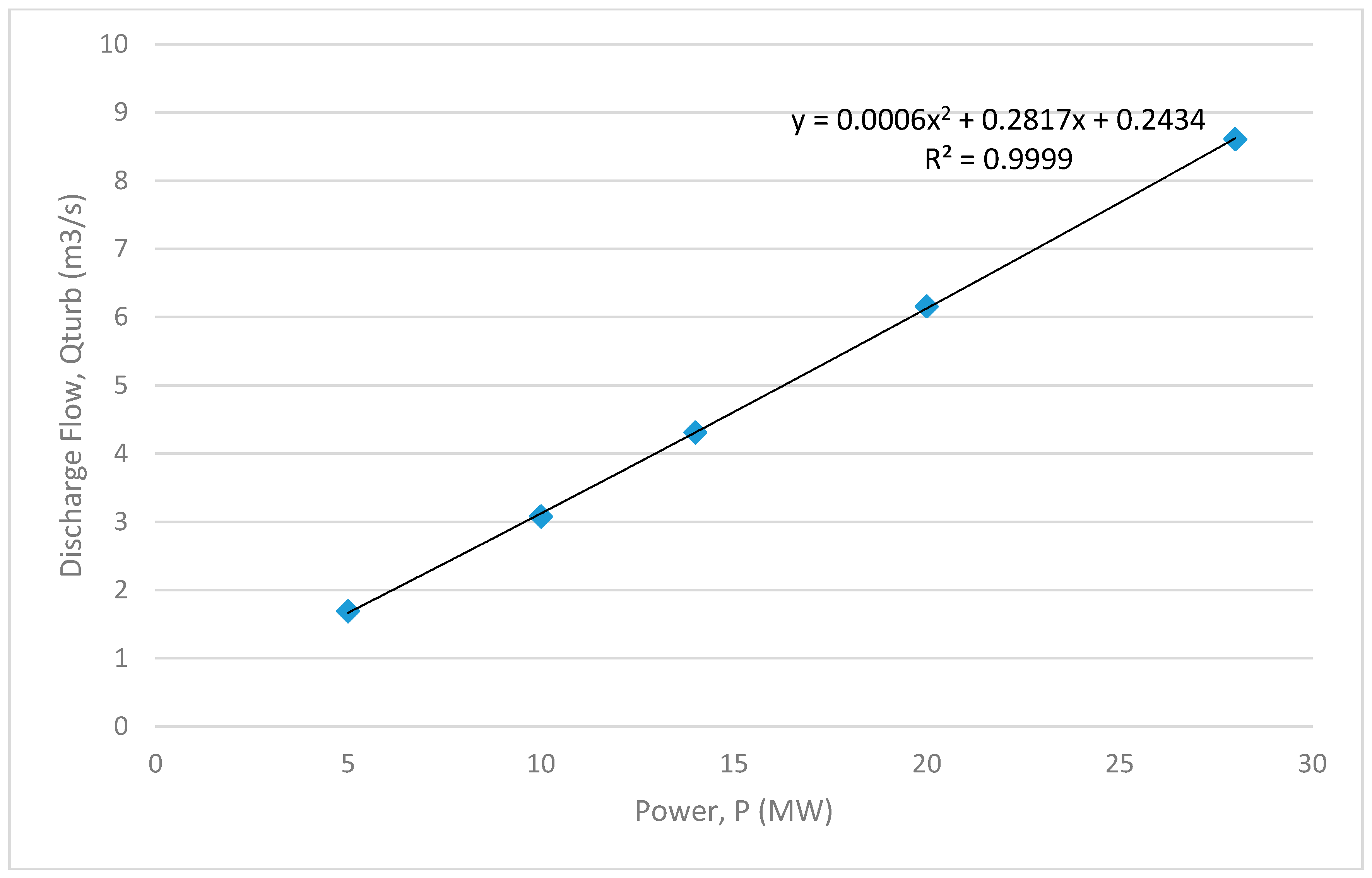
As for the turbine discharge flow, Qturb for each turbine can be computed if the power output of generator unit is known. The turbine discharge had been obtained by studying the turbine characteristics provided by manufacturers and recent performance tests. The relationship between turbine discharge flows versus power outputs is as given in Table 2. Using Table 2, one can plot a relationship curve between turbine discharges versus generator power outputs (as in Figure 6), also to find their relationship, as in Equation (7):
P is power output in MW driven by the turbine. In Equation (7), turbine discharge flow is a function of generated power as gross head and efficiency remain almost constant when the generator output is greater than 10 MW, as tabulated in Table 2.
The relationship as plotted in Figure 6 seems to be linear, but it is not, as the coefficient for the (P)2 term in Equation (7) is not zero but 0.0006. The nonlinear characteristic of the plot can be shown by investigating the same correlation in dimensionless form, i.e., overall efficiencies as in Equation (8); (the overall efficiency depends on relationships between generator power, gross head and turbine discharge flow):
where generator load (W); water density (kg/m3); gravitational acceleration (m/s2); gross head (m); turbine discharge (m3/s).
As an example, using the data for 5 MW in Table 2, and let = 997 kg/m3, Hg = 403 m, g = 9.781 m/s2 (is typical value of g for Malaysia), with turbine discharge equals to 1.69 (Qturb = 1.69 m3/s), yields the following efficiency:
The remaining computed efficiency results are tabulated in Table 2. Overall efficiency at 5 MW is significantly low since the number of operating nozzles is either two or four. While each nozzle was designed to work best at values between 5 and 7.5 MW, utilizing two nozzles for generator output as low as 5 MW made each nozzle to operate at 2.5 MW, which is far below its best design load. As the load per nozzle exceeds 5 MW, its efficiency reaches almost the flat zone. This is the important contributing factor why overall efficiency has achieved almost a constant value beyond this load.
Though the two generating units in this plant do not have identical turbine discharge and overall efficiency characteristics, however for a purpose of simplification, in this project they have been considered similar (turbine discharge versus generator output and overall efficiency versus generator outputs curves).
All these computations has been realized in the form of ladder logic rungs on a programmable logic controller (PLC). In summary, the average river flow is the right hand-side component of Equation (4) divided by time integration interval.
4. Turbine Control Algorithms
Level-based controllers that employed PI and PID for run-off river hydropower have been studied by many groups [8,9,10,11,12]. Others have investigated applications of fuzzy logic to regulate small hydroelectric systems [13,14]. Unlike the level-based controllers, the newly proposed method improves control of hydroelectric turbines by employing controllers that regulate according to the mass flow rates of rivers. The flow rate is not measured but derived mathematically from parameters collected from the existing sensors at the plants. The computed flow rate is then used to compute turbine set points to regulate the power output of turbines.
If the controller knows an additional amount of water will arrive ahead of time, it should increase the set points to deliver more water to the turbines to reduce future spillages (assuming the present water level is at the crest of the dam). To know the volume of water that will arrive ahead of time requires measurement of upstream river flow, consequently requiring the installation of telemetry and sensors, and therefore it is not within scope of this project.
4.1. Proposed Turbine Controller Set Point Computation
If the water level is at the targeted level, then the turbine set point is the river flow if both the river flow and turbine discharges are stable over a period of time. However if the water level is higher or lower than the targeted level, than the turbine set point is no longer the computed river flow. The turbine set point is rather the summation of river flow plus the amount of water in the pond that needs to be delivered to the turbines to reduce spillage, as depicted in Figure 7.
The difference between the targeted water level and present water level can be either positive or negative; therefore the set point (named as optimum flow (Qopt) can either be greater or lesser than the river flow.
Figure 7 can be represented as Equation (9) to compute the optimum flow as turbine set point. The target water (WLtr) is the water level set point to achieve, and its value needs to be entered into the control system manually by an operator via a human machine interface:
where = targeted dam water level (mSLE); = current dam water level (mSLE) after ; = average water surface area for intake pond (m2); = final time for the control regulation interval (s).
4.2. Turbine Discharge Flow Allocation Turbine Controller
Similar to other computations, Equation (9) have been implemented as PLC ladder logic. The integration time has been adopted as the control regulation intervals at this hydroelectric system. All flows need to be computed within the regulation period, which in our case is five minutes.
After the river flow and optimal flow computations, the controller continues to allocate the optimal flow to either both turbines or only one turbine, determining their operating set points, depending on the magnitude of river flow as depicted in Figure 8.
The allocation of available flow also depends on the availability of each turbine. If both turbines are available and on auto mode, the controller may divide the optimal flow equally, thus both turbines will have equal set point flows. Alternatively, the controller should load the most efficient turbine to the maximum, and the reminder of the optimum flow goes to the next one. As the river flow increases or decreases, the controller decides to run either both turbines or one only. Running two turbines incurs two sets of auxiliary power needed by both units. The summary of sequences by the controller is as follows:
- (a)
- To determine optimal plant discharge Qopt, using the mass balance method, with intake water elevation as one of the inputs as described previously in Section 4.1.
- (b)
- Next step (as shown in Figure 8) is to compute the effective optimal flow (Qopt*). Qopt* is equal to deduction of Qopt by a value determined by the conditions of trash racks. The trash rack penalty starts when the trash rack differential pressure (DP) in terms of water level difference is greater than 40 cm.
- (c)
- Subsequent steps are to maximize energy production for a given Qopt* to both turbines, according to their availability status, auto/manual modes and efficiencies as follows:
- Depending on the magnitude of the calculated effective optimal flow (Qopt*), the controller determines the number of units: N (either N = 1 unit or N = 2 units of turbines) that are able to be loaded up.
- If only one unit is available (N = 1; unit availability is determined via circuit breaker status), load the available unit either to its maximum energy output or flow rating equal to Qopt*, whichever is lower. Since the unit available can be either the unit 1 or unit 2 turbine, the Qopt* should be allocated to the appropriate available turbine.
- If one of the turbines is in manual mode, the controller needs to subtract the flow amount belonging to the turbine in manual mode from the Qopt*. The subtraction result then becomes the set point flow for the turbine in auto mode.
- If two units of turbines are available (N = 2), and both are in auto mode, the controller allocates Qopt* according to:
- -
- In case Qopt* ≥ (Qmax/number of turbines), then load both turbine units to their maximum rating, where Qmax is the flow of turbine to produce the maximum power.
- -
- In case Qopt* < (Qmax/number of unit), then in this case Qopt* is not sufficient to load up both units to their maximum capacities. Therefore the controller needs to load either one unit only or two units depending on criteria such as auxiliary power consumptions and turbine efficiencies. Two running turbines need almost double amount of auxiliary power compared to that required for one in service. As river flow varies, the controller should shut down one unit (either unit 1 or 2 turbine) when the river flow becomes low.
4.3. Turbine Control Protections
In addition to the computations and logic sequences described previously, the controller needs to be equipped with multiple interlocks to protect the turbines in case abnormal conditions occur. Examples of abnormal conditions are sudden water level drops, unusually high pressure differentials across trash racks, and turbine nozzle complications. The limits or data employed in abnormal conditions have been established from calculations, turbine manufacturer specifications, experiments and tests performed.
A sudden water level drop will occur when the upper station trips, as water that is normally discharging from the upper station is no longer directly entering into the lower hydroelectric penstock. Instead, the water will be diverted into one of tributaries, causing the lower station to suffer deprivation of seventy percent of its total water flow for up to a few hours. To detect sudden drops of water level, simpler and fast computation has been developed. Rather than employing a flow computation method, the controller detects consistently multiple level drops with each drop greater than a certain magnitude for certain duration, as in Equation (10):
Each level difference is measured in 10 s for at least a total duration of 3 min. If the condition in Equation (10) is true, the controller will reduce both turbines to 7 MW power outputs. Further de-loads occur if the water level keeps decreasing very fast. This criterion is adopted to avoid false events and ensure a sudden drop of water level did occur, whereby multiple water level decrements need to be observed, with each drop greater than 0.005 m happening in a 10 s period. In other words, the sudden water drop is confirmed, if level drops are detected in consecutive ten second periods with each drop being greater than 0.005 m, for a total observation over 3 min that the total drop reaches 0.1 m or greater.
When the trash rack’s differential pressure is very high, once the water level (at the post-trash rack location) is lower than 534.12 m, the controller will start to reduce both turbines’ load to 7 MW. As for abnormal turbine nozzle conditions, the controller establishes this condition when there is a difference of greater than 0.15 MW between its command and load reference. This means its command does not go through. If a raising command has been issued three times, but the turbine’s load does not change, the controller will jump to manual mode.
5. Controller’s Hardware and Software
Implementations of controllers on programmable logic controller (PLC) can be found in many references [15,16,17,18,19]. PLCs are easy to program and popular as controllers to serve power generation systems. Therefore the selected hardware and software platform for the proposed controller should be PLC, and a SIEMENS S7-300 model (Erlangen, Germany) had been chosen. To enable operator to control and monitor the turbines, graphics such as controller command buttons, data value entries or constant data and trending had been created on a human machine interface (HMI).
5.1. Programmable Logic Controller (PLC)
The picture of implemented controller on the SIEMENS PLC is as in Figure 9. The PLC has input modules to acquire plant parameters either directly from the fields (such as the new water level sensor), or from remote terminal units (RTUs) of the existing supervisory control and data acquisition (SCADA) system, or electrical cabinets.
The PLC has output modules with interposing relays for digital inputs and outputs needed for status inputs, command outputs and alarms. The SIEMENS PLC S7-300 (Erlangen, Germany) has been chosen due to its robustness for power station applications and that fact it possesses many different types of timers with the high resolution and sufficiently long duration needed for this project [20]. Those timers have been utilized for sampling intervals, numerical integration periods as well time pulses for energizing turbine servomotors. Energizing a servomotor requires multiple timers either to increase or decrease turbine flows, or for sudden flow reduction when abnormalities do occur.
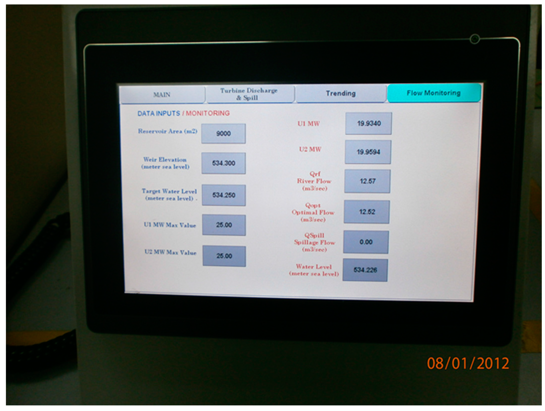
5.2. Human Machine Interface (HMI)
A picture of the HMI is as shown in Figure 10. The HMI with a touch screen provides facilities for operators to either initiate commands or enter coefficients or target water levels. Examples of coefficients are the floating constants needed by flow computations. Control buttons allow operators to put the controller into auto or manual mode that the appropriate memory bits within the PLC will be set or reset, and command buttons to raise or lower turbine discharge as well as entries for maximum limits of generator power outputs. Also, monitoring of crucial parameters and trending are among the pages included on the HMI.
6. Commissioning Results
Commissioning tests had been conducted to evaluate correctness of river flow computations, control system protection interlocks, and ability of controller either to raise or lower the turbine’s load within selected control intervals.
6.1. Flow Computations & Turbine Controller
Samples of river flow computation, optimum flow and spillages is as tabulated in Table 3, which indicates that the optimum flows should be higher than the river flows as the controller attempted to reduce spillages.
The commissioning tests to prove the controller can raises load is shown in Table 4. The controller raised power outputs for both turbines by raising the load settings, therefore the power outputs from both generators increased. Total power outputs for both generators as shown increased from 37.8 MW to about 44.0 MW. Also, Table 4 indicates that as the total power increased, the intake pond water levels (measured in meters above sea level elevation (mSLE) decreased accordingly as the river flow remains unchanged.
Table 5 is a snapshot of the controller maintaining the magnitude of power output with river flow lesser than the turbine flow, causing water levels to drop.
6.2. Assessment of Energy Production Improvement
Table 6 shows operation data for the lower cascade hydropower plant for a duration of 174 days from January to June 2013. From the table it can be seen that the total incoming flow available was 195.3 million cubic meters. The plant owner had set the maximum limit that the plant could handle at 102.5 million cubic meters, due to many factors, including the generating units’ recent performance. Using these figures and Equation (11), the measurement for water utilization effectiveness (WUE) in percentage can be calculated:
If one evaluates Equation (10), it yields 100% for perfect water utilization, i.e., accounted spillage is zero and 0% for zero utilization rate or 100% spilled. For incoming flow of 195.3 × 10⁶ m3 and accounted spillage of 23.11 × 10⁶ m3, initial WUE is as follows:
Table 7 shows operation data for the same plant from 24 July to 23 September 2013. Total duration was 90 days with the new controller online most of the time. From the table it can be seen that the total available incoming flow was 35.1 million cubic meters. The plant owner had set the maximum limit for the plant at 65.2 million cubic meters due to the same factors as before. The accounted spillage was 1.76 million cubic meters. Using Equation (11), therefore the plant WUE with the new controller becomes:
It can be seen the WUE with the new controller for this plant has increased significantly from 88.17% to 97.12%, indicating a higher fraction of the incoming flow went to the generating units rather than over the spillway crest. Generation improvement can be represented by the reduction of accounted generation lost from the two tables normalized for the same duration. The calculations are as the follows:
- (a)
- Initial accounted generation lost = 19,665 MWh
- (b)
- Duration = 174 days
- (c)
- Initial accounted lost/day = 113.2 MWh
Repeating the same procedure, now using data from Table 7:
- (a)
- Accounted generation lost = 776 MWh
- (b)
- Duration = 61 days
- (c)
- Initial accounted lost/day = 12.7 MWh
Therefore the generation improvement is by 100.3 MWh/day or 36,608 MWh/year. Taking the conservative estimate that the average cost to produce one MWh for this country at 38 USD, then the estimated annual savings associated with these figures is 1.39 million USD /year.
7. Conclusions
In this paper, a novel computational method to obtain river flows for a run-off river hydroelectric system has been presented. This simple computational method is based on conservation of mass whereby water entering the intake pond equals the water being stored and released. The incoming water is the river flow, while the rise and fall of water levels at the pond represent water being stored, and water is released in the forms of spillages and turbine discharges.
Mathematically, the average of river flow is derived by dividing a summation of pertinent water volume changes by an integration interval. The pertinent volume change is the summation of pond volume change with numerical integration of both turbine discharge flow and spillages.
Instead of installing flow sensors to measure river flows, this elegant method takes advantage of existing power meter devices and the accuracy of water level sensors. Periodic measurement of water level sensors at integration period intervals provides a height difference for computing the pond’s volume changes (since the geometrical shape of pond is known). Similarly water level measurements with the selected time resolution allows derivation of spillages, as spillages are a function of water levels above the dam crest. As for the turbine discharges, it can be derived from the power outputs for most range of generator outputs as turbine efficiency and gross heads remain almost constant for the Pelton turbines in this hydroelectric system.
Subsequent to the computation of average river flow, the controller computes turbine set points defined as optimal flows. An optimal turbine discharge flow is not necessarily equal to the river flow, but it is summation of present river flow plus accumulated excess water in the intake pond to reduce spillages. Therefore more energy can be produced instead of being wasted as spillages. Opposite to spillages, lack of water in the pond should cause the set point to be lower than the present river flow as water level needs to be raised to an appropriate level, especially at high turbine loads.
Knowledge of river flows allows the controller to decide the number of turbines in service easily as the discharge flow and relative efficiency of each turbine are known. Either running the most efficient turbine or two turbines to the maximum rating or shutting down one turbine to save total auxiliary power are therefore easily implemented.
All the computations, control sequences and turbine protection interlocks has been realized as ladder logics on a SIEMENS programmable logic controller. Also all the computations, protection logics and control schemes had been verified manually and tested during the commissioning periods.
As the controller has stable control responses while in operation with the successful commissioning tests performed, and energy production assessments made in Section 6, though for short observation months, it can be concluded that the suggested methods of computing river flow and turbine set points have been successful to reduce spillages. It is therefore able to improve energy production of the hydroelectric system selected for this research.
Acknowledgments
The authors would like to thank TNB generation department and Sg. Perak hydro-electric station management for funding this research. Also appreciation goes to the Sg. Piah and Bersia control center personnel for their support and cooperation.
Author Contributions
Both authors contributed equally to the work, with Abdul Bahari Othman focusing on the mechanical engineering scopes, while Razali Jidin dedicated his time more on the control system and wrote most parts of this paper.
Conflicts of Interest
The funding agency had no role in the design or result of this study; in the collection, analyses, or interpretation of data; in the writing of the manuscript, and in the decision to publish the results.
References
- Marsh, T. Capitalising on river flow data to meet changing national needs—A UK perspective. Flow Meas. Instrum. 2002, 13, 291–298. [Google Scholar] [CrossRef]
- Creutin, J.; Muste, M.; Bradley, A.; Kim, S.; Kruger, A. River gauging using PIV techniques: A proof of concept experiment on the Iowa River. J. Hydrol. 2003, 277, 182–194. [Google Scholar] [CrossRef]
- Muste, M.; Ho, H.; Kim, D. Considerations on direct stream flow measurements using video imagery: Outlook and research needs. J. Hydro-Environ. Res. 2011, 5, 289–300. [Google Scholar] [CrossRef]
- Yorke, T.; Oberg, K. Measuring river velocity and discharge with acoustic Doppler profilers. Flow Meas. Instrum. 2002, 13, 191–195. [Google Scholar] [CrossRef]
- Mwakalila, S. Estimation of stream flows of ungauged catchments for river basin management. Phys. Chem. Earth Parts A/B/C 2003, 28, 935–942. [Google Scholar] [CrossRef]
- Fasol, K. A short history of hydropower control. IEEE Control Syst. Mag. 2002, 22, 68–76. [Google Scholar] [CrossRef]
- Loosemore, W. Ultrasonic river flow measurement. Ultrasonic 1973, 11, 195–196. [Google Scholar] [CrossRef]
- Sarasua, J.I.; Fraile-Ardanuy, J.; Perez, J.I.; Wilhelmi, J.R.; Sanchez, J.A. Control of a run of river small hydro power plant. In Proceedings of the 2007 International Conference on Power Engineering, Energy and Electrical Drives, Setubal, Portugal, 12–14 April 2007. [Google Scholar]
- Natarajan, K. Robust PID Controller Design for Hydro-turbines. IEEE Trans. Energy Convers. 2005, 20, 661–667. [Google Scholar] [CrossRef]
- Frick, P.A. Automatic control of small hydroelectric plants. IEEE Trans. Power Appar. Syst. 1981, 100, 2476–2485. [Google Scholar] [CrossRef]
- Endo, S.; Konishi, M.; Imabayasi, H. Water level control of small-scale hydroelectric power plant by deadbeat control method. In Proceedings of the 26th Annual Conference of IEEE Industrial Electronics Society (IECON 2000), Nagoya, Japan, 22–28 October 2000; pp. 1123–1128. [Google Scholar]
- Dumur, D.; Libaux, A.; Boucher, P. Robust control for Basse-Isere run-of-river cascade hydroelectric plants. In Proceedings of the IEEE International Conference on Control Applications (CCA’01), Mexico City, Mexico, 7 September 2001; pp. 1083–1088. [Google Scholar]
- Yadav, O.; Kishor, N.; Fraile-Ardanuy, J.; Mohanty, S.R.; Perez, J.I.; Sarasua, J.I. Pond head level control in a run-of-river hydro power plant using fuzzy controller. In Proceedings of the 16th International Conference on Intelligent System Applications to Power Systems, Hersonissos, Greece, 25–28 September 2011; pp. 1–5. [Google Scholar]
- Priyadharson, A.; Ganesan, R.; Surarapu, P. PLC-HMI Automation Based Cascaded Fuzzy PID for Efficient Energy Management and Storage in Real Time Performance of a Hydro Electric Pumped Storage Power Plant. Procedia Technol. 2015, 21, 248–255. [Google Scholar] [CrossRef]
- Gerkšič, S.; Dolanc, G.; Vrančić, D.; Kocijan, J.; Strmčnik, S.; Blažič, S.; Škrjanc, I.; Marinšek, Z.; Božiček, M.; Stathaki, A.; et al. Advanced control algorithms embedded in a programmable logic controller. Control Eng. Pract. 2006, 14, 935–948. [Google Scholar] [CrossRef]
- Góra, P.; Sroczan, E.; Urbaniak, A. Programmable Logic Control (PLC) for Small Water Demineralization Plant. IFAC Proc. Vol. 1992, 25, 251–256. [Google Scholar] [CrossRef]
- Alphonsus, E.; Abdullah, M. A review on the applications of programmable logic controllers (PLCs). Renew. Sustain. Energy Rev. 2016, 60, 1185–1205. [Google Scholar] [CrossRef]
- Shilin, A.; Savrasov, F.; Kriger, A. A methodology for the construction of efficient PLC based low-power photovoltaic generation plants. Resour. Effic. Technol. 2016, 2, 105–110. [Google Scholar] [CrossRef]
- Li, J.; Liu, L.Q.; Xu, X.D.; Liu, T.; Li, Q.; Hu, Z.J.; Wang, B.M.; Xiong, L.Y.; Dong, B.; Yan, T. Development of a Measurement and Control System for a 40l/h Helium Liquefier based on Siemens PLC S7-300. Phys. Procedia 2015, 67, 1181–1186. [Google Scholar] [CrossRef]
- SIEMENS. SIMATIC Ladder Logic (LAD) for S7-300 and S7-400 Programming; Reference Manual, 6ES7810-4CA10-8BW1, 05/2010; SIEMENS: Erlangen, Germany, 2011. [Google Scholar]
Figure 1.
Cascaded run-off river hydroelectric system (upper and lower station).
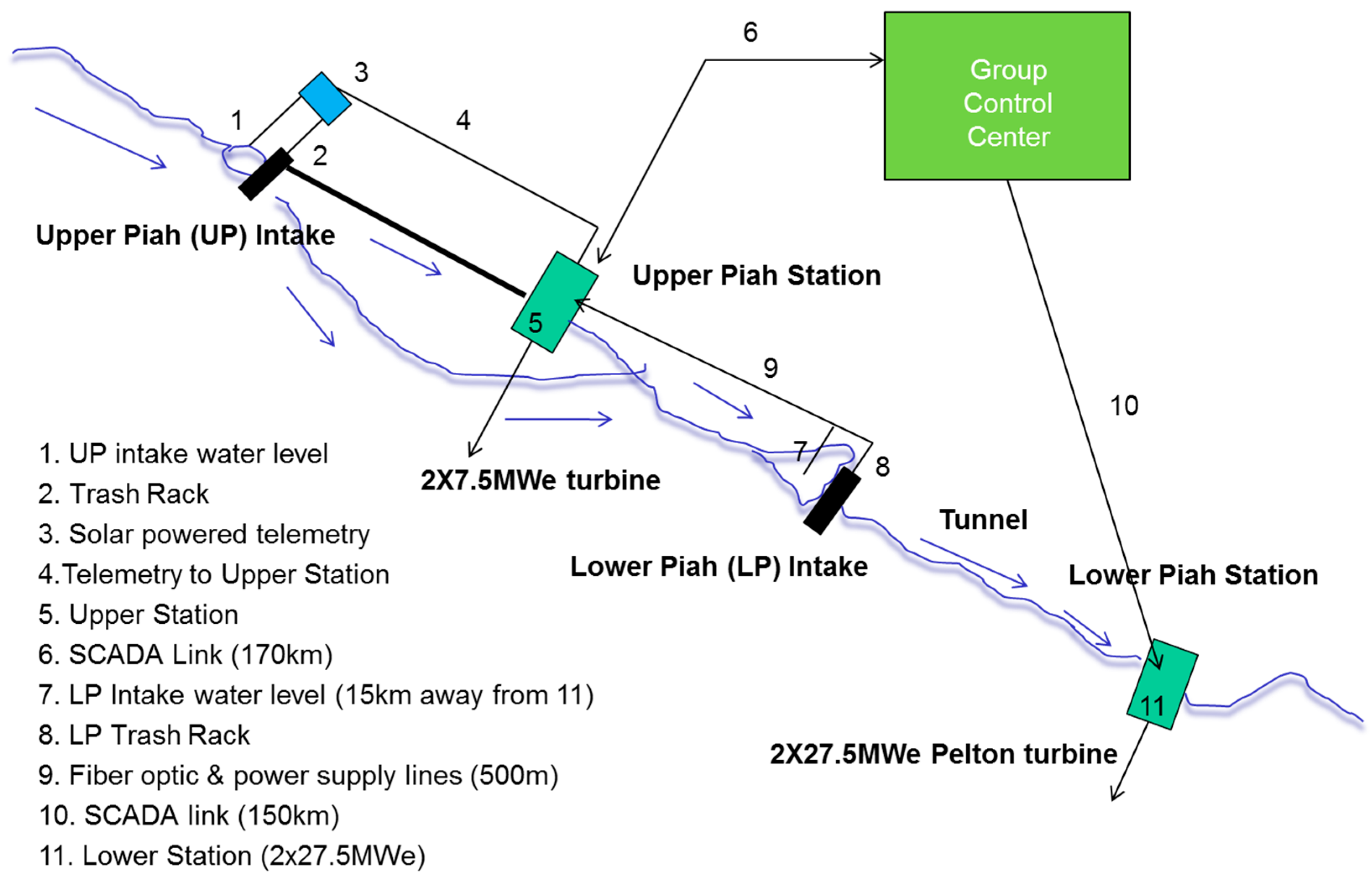
Figure 2.
Lower hydroelectric intake pond with spillage.
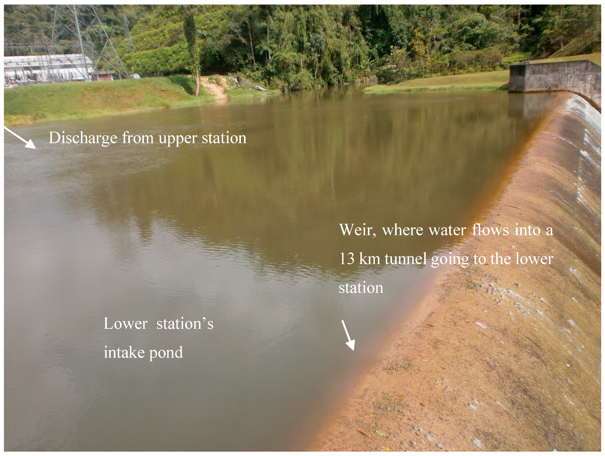
Figure 3.
River flow as summation of flows and pond volume rate.

Figure 4.
River flow as summation of turbine discharge, spillage and pond volume rate.

Figure 5.
Spillage versus Delta H.

Figure 6.
Turbine discharge derived from generator power output.

Figure 7.
Calculation of turbine discharge flow set point (Qopt).
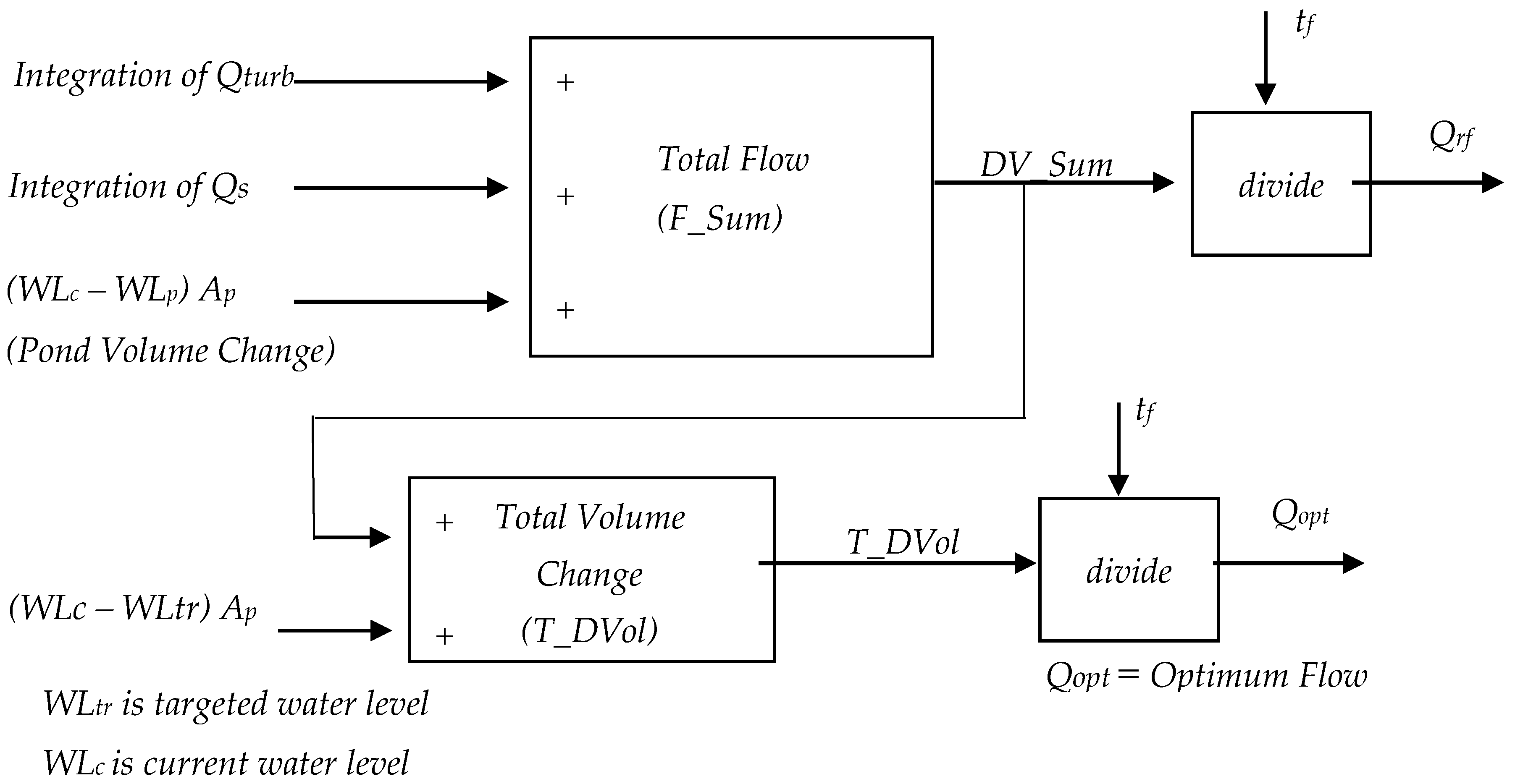
Figure 8.
Discharge flow set point algorithm & simplified controller commands.
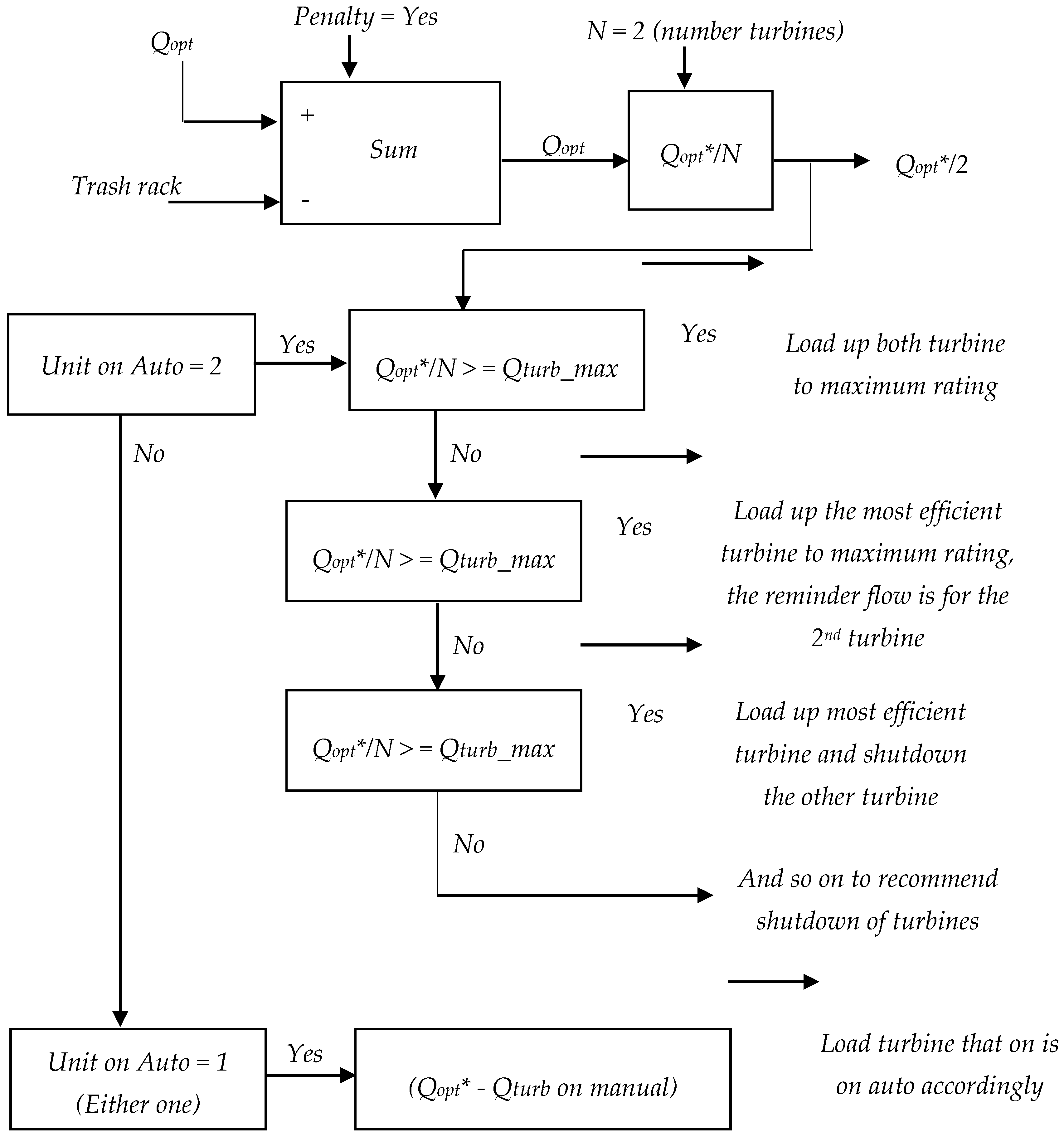
Figure 9.
Programmer logic controller (PLC).
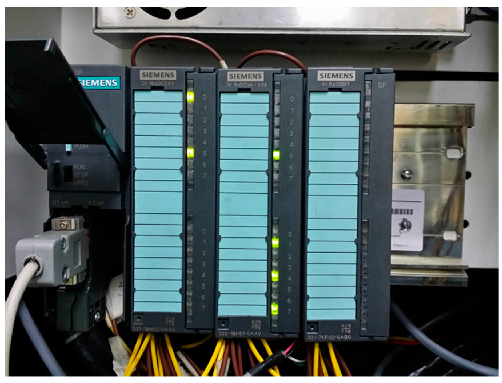
Figure 10.
HMI: a sample of HMI graphic page.


Table 1.
Spillage versus delta H.
| Fore-Bay Elevation, FBE (mSLE) | Delta H, DH (m) | Spillage, Qspill m3/s |
|---|---|---|
| 534.32 | 0.00 | 0.0 |
| 534.33 | 0.01 | 1.0 |
| 534.34 | 0.02 | 2.2 |
| 534.35 | 0.03 | 3.3 |
| 534.36 | 0.04 | 4.5 |
| 534.37 | 0.05 | 6.1 |
| 534.38 | 0.06 | 7.8 |
| 534.39 | 0.07 | 13.0 |
| 534.4 | 0.08 | 15.3 |
| 534.43 | 0.11 | 16.0 |
| 534.44 | 0.12 | 16.0 |
Table 2.
Turbine Discharge Flow Derived from Generator Power.
| Generator Power, P | Number of Nozzles | Gross Head *, Hg (m) | Total Turbine Discharge, Qturb | Overall Efficiency, ηo |
|---|---|---|---|---|
| 5.0 | 2 | 403 | 1.69 | 75.28 |
| 10.0 | 2 | 403 | 3.08 | 82.62 |
| 14.0 | 4 | 403 | 4.31 | 82.65 |
| 20.0 | 4 | 403 | 6.16 | 82.62 |
| 28.0 | 4 | 403 | 8.61 | 82.75 |
* Variation of intake water level (<0.75 m) relative to gross head is small. Thus overall efficiency can be approximate as function generator power output only.
Table 3.
Samples of river flows, optimum flows and spillages.
| Qrf (m3/s) | Qopt (m3/s) | Qspill (m3/s) |
|---|---|---|
| 19.97 | 20.19 | 4.22 |
| 19.83 | 20.05 | 3.49 |
| 18.83 | 19.02 | 3.04 |
Table 4.
Snapshots of controller raising the load to reduce spillages.
| Time | Unit 1 Load Setting (%) | Generator (MW) | Unit 2 Load Setting (%) | Generator (MW) | Water Level (mSLE) | Generator Total (MW) |
|---|---|---|---|---|---|---|
| 11:10 h | - | 19.0 | - | 18.8 | - | 37.8 |
| 11:30 h | 57 | 20.3 | 69 | 21.0 | 534.47 | 41.3 |
| 11:40 h | 57 | 20.4 | 69 | 20.9 | 534.47 | 41.3 |
| 11:50 h | 57 | 20.4 | 69 | 21.0 | 534.46 | 41.4 |
| 12:00 h | 62 | 21.9 | 72 | 22.1 | 534.45 | 44.0 |
| 12:10 h | 62 | 21.9 | 72 | 22.1 | 534.45 | 44.0 |
| 12:20 h | 62 | 21.8 | 72 | 22.0 | 534.46 | 43.8 |
Table 5.
Snapshots of controller maintaining a high load with reducing water level.
| Time | Unit 1 Load Setting (%) | Generator (MW) | Unit 2 Load Setting (%) | Generator (MW) | Water Level (mSLE) | Generator Total * (MW) |
|---|---|---|---|---|---|---|
| 21:30 h | 74 | 25.3 | 72 | 21.7 | 534.41 | 47.0 |
| 21:40 h | 74 | 25.3 | 72 | 21.7 | 534.40 | 47.0 |
| 21:50 h | 74 | 25.3 | 72 | 21.7 | 534.38 | 47.0 |
| 22:00 h | 74 | 25.3 | 72 | 21.7 | 534.37 | 47.0 |
| 22:10 h | 74 | 25.3 | 72 | 22.7 | 534.38 | 47.0 |
| 22:20 h | 74 | 25.3 | 72 | 21.7 | 534.36 | 47.0 |
| 22:30 h | 74 | 25.4 | 72 | 21.7 | 534.35 | 47.1 |
| 22:40 h | 74 | 25.4 | 72 | 21.7 | 534.37 | 47.1 |
| 22:50 h | 74 | 25.4 | 72 | 21.7 | 534.36 | 47.1 |
| 23:00 h | 74 | 25.4 | 72 | 21.7 | 534.36 | 47.1 |
* Note: The maximum load of 47.1 MW differs from the rated design of 55 MW due to limitation imposed or plant conditions.
Table 6.
Generation data prior to utilization of the new controller (3 January–6 June 2013).
| Month | Number of Days | Incoming Flow (×106 m3) | Actual Plant Discharge (×106 m3) | Max. Discharge Limit (×106 m3) | Accounted Spillage (×106 m3) | Accounted Generation Lost (MWh) |
|---|---|---|---|---|---|---|
| January | 23* | 29.88 | 14.66 | 17.74 | 3.08 | 2620 |
| February | 23* | 23.14 | 14.48 | 17.28 | 2.79 | 2378 |
| March | 31 | 26.00 | 17.00 | 22.46 | 5.46 | 4643 |
| April | 30 | 28.64 | 17.16 | 22.07 | 4.91 | 4174 |
| May | 31 | 62.40 | 19.00 | 22.51 | 3.50 | 2982 |
| June | 30 | 20.81 | 16.27 | 19.40 | 3.13 | 2664 |
| July | 6 | 4.38 | 3.96 | 4.20 | 0.24 | 205 |
| Total | 174 | 195.3 | 102.5 | 125.7 | 23.11 | 19,665 |
Table 7.
Generation data after installation of the computed river flow-based controller (24 July to 23 September 2013).
Table 7.
Generation data after installation of the computed river flow-based controller (24 July to 23 September 2013).
| Month | Number of Days | Incoming Flow (×106 m3) | Actual Plant Discharge (×106 m3) | Max Discharge Limit (×106 m3) | Accounted Spillage (×106 m3) | Accounted Generation Lost (MWh) |
|---|---|---|---|---|---|---|
| July | 7 | 3.60 | 3.38 | 6.98 | 0.21 | 93 |
| August | 31 | 16.97 | 13.80 | 30.77 | 0.95 | 423 |
| September | 23 | 14.55 | 12.88 | 27.42 | 0.59 | 261 |
| Total | 61 | 35.1 | 30.0 | 65.20 | 1.78 | 776 |
© 2017 by the authors. Licensee MDPI, Basel, Switzerland. This article is an open access article distributed under the terms and conditions of the Creative Commons Attribution (CC BY) license (http://creativecommons.org/licenses/by/4.0/).
Share and Cite
MDPI and ACS Style
Jidin, R.; Othman, A.B. A Computed River Flow-Based Turbine Controller on a Programmable Logic Controller for Run-Off River Hydroelectric Systems. Energies 2017, 10, 1717. https://doi.org/10.3390/en10111717
AMA Style
Jidin R, Othman AB. A Computed River Flow-Based Turbine Controller on a Programmable Logic Controller for Run-Off River Hydroelectric Systems. Energies. 2017; 10(11):1717. https://doi.org/10.3390/en10111717
Chicago/Turabian StyleJidin, Razali, and Abdul Bahari Othman. 2017. "A Computed River Flow-Based Turbine Controller on a Programmable Logic Controller for Run-Off River Hydroelectric Systems" Energies 10, no. 11: 1717. https://doi.org/10.3390/en10111717
Note that from the first issue of 2016, this journal uses article numbers instead of page numbers. See further details here.