Improved Load Frequency Control Using a Fast Acting Active Disturbance Rejection Controller


1
Department of Electrical and Electronic Engineering, Dhaka University of Engineering and Technology, Gazipur1700, Bangladesh
2
Department of Electrical and Electronic Engineering, Bangladesh University of Engineering and Technology, Dhaka1205, Bangladesh
3
School of Engineering and Information Technology, University of New South Wales-Canberra, Northcott Dr, Campbell ACT 2612, Australia
*
Author to whom correspondence should be addressed.
Energies 2017, 10(11), 1718; https://doi.org/10.3390/en10111718
Submission received: 6 September 2017
/
Revised: 12 October 2017
/
Accepted: 23 October 2017
/
Published: 27 October 2017
(This article belongs to the Section F: Electrical Engineering)
Abstract
:System frequency may change from defined values while transmitting power from one area to another in an interconnected power system due to various reasons such as load changes and faults. This frequency change causes a frequency error in the system. However, the system frequency should always be maintained close to the nominal value even in the presence of model uncertainties and physical constraints. This paper proposes an Active Disturbance Rejection Controller (ADRC)-based load frequency control (LFC) of an interconnected power system. The controller incorporates effects of generator inertia and generator electrical proximity to the point of disturbances. The proposed controller reduces the magnitude error of the area control error (ACE) of an interconnected power system compared to the standard controller. The simulation results verify the effectiveness of proposed ADRC in the application of LFC of an interconnected power system.
1. Introduction
Satisfactory operation of a power system involves both active and reactive power- balance between generation and load. These balances drive two equilibrium points: frequency and voltage. Stable operation of interconnected power system requires both acceptable frequency and tie-line power exchange [1]. Load frequency control (LFC), which is mainly used to maintain the standard frequency and the tie-line power exchange under schedule during any load changing event, can be defined as regulation of active power and frequency [2]. As the regulated output of the LFC, an area control error (ACE) that has a linear relationship between tie line power and frequency deviation is considered. Basically, LFC is responsible for controlling ACE zero and to do this, frequency and tie-line power errors need to be zeros.
There are a number of decentralized LFCs in the literature; however, Proportional Integral Derivative (PID) control is the most widely used in power industry [3,4,5,6]. Although PID controllers are widely employed in industry for their simplicity in implementation, their primary hinderances are large frequency deviation and long settling time (about 10 to 20 s) during disturbances [7]. In [8] four fundamental technical limitations in the existing PID framework are mentioned, including the following: (1) the error computation; (2) noise degradation in the derivative control; (3) over simplification and the performance loss; and (4) integral term control complications.
The corresponding technical and conceptual solutions of an ADRC-based control system instead of a PID-based control system are proposed in [8].The four fundamental limitations of PID controllers can be resolved by introducing the following four characteristics: (1) a differential equation need to be added; (2) a differentiator for noise-tolerant tracking; (3) the total disturbance rejection and estimation; and (4) the power of nonlinear control feedback.
Fuzzy logic based decentralized LFC is widely applied in [9,10,11,12]. Specifically, a fuzzy logic controller, developed directly from a fuzzy model of the power system, is proposed in [9]. A fuzzy logic based tie-line bias control scheme on a two-area multiple-unit power system is introduced in [10]. The comparisons between fuzzy logic and conventional PID control techniques are presented for a combined cycle power plant in [11]. In the Iraqi National Super Grid power system, a fuzzy gain-scheduled Proportional Integral (PI) controller and its execution is implemented in [12]. Such a controller is often combined with PI or PID controllers to optimally adjust PID gains. PI controllers have been broadly used for decades in industry as the load frequency controllers. A model-following controller for multiple-input multiple-output (MIMO) systems is presented in [13]. A PI controller, which is tuned through genetic algorithm linear matrix inequalities (GALMI), is demonstrated for LFC in a nine-unit power system for three areas [14]. A high-order learning control law terminal iterative learning control (TILC) is developed to improve control performance. The new developed control law is a data-driven control strategy, where any other model information of the control plant do not need except for the I/O measurements [15]. The model-free sliding mode controllers have been applied to control the azimuth and pitch positions in two single input single output control loops and it has proved its effectiveness over intelligent PI control system [16]. The ADRC technique is adopted to resolve the output power variation of wind turbines in the sub-controllers’ switching process. The switching transition of output power is reduced using ADRC and the system’s performance is improved [17].
In recent years, active disturbance rejection control (ADRC), developed by Han in 1995 [18] and modified by Gao [18,19,20], is proposed for the LFC controller [21,22,23]. It is an emerging controller that estimates and mitigates uncertainties internally and externally in real time. For these reasons ADRC controller is often seen to apply in power systems. The basic idea of ADRC is that it uses an Extended State Observer (ESO) for estimating and cancelling the disturbances of the system for simplification of the control problem. The design process of the controller is simple that does not need an accurate system model. This controller, showing robustness during sudden disturbances and structural uncertainties, can be used as decentralized [24].
ADRC is implemented for LFC on an interconnected power system in [25,26,27,28]. This controller for LFC is studied in the Bangladesh Power System (BPS) [25]. ADRC and PI-Fuzzy compound controller are proposed and applied for the current compensation of Active Power Filters [26]. In addition, the ADRC is revealed to be superior to the existing GALMI tuned PI controller in smaller ACE and ∆f and faster response of the closed-loop system. A novel design of a robust decentralized LFC is proposed for an interconnected power system in [27]. Moreover, the effects of system parameter variations on ACE, frequency error and tie-line power error, are also reported. The ADRC is modified using a Repetitive Controller (RC) and applied to a power system with two different turbine units in [28] enhancing the performance of ADRC as a controller. A coordinated controller based on multivariable predictive control theory is presented to demonstrate its effectiveness during variable operation with unpredictable renewable energy generation and load changes in [29]. For the application of current compensation of active power filter, ADRC and PI-fuzzy are proposed n [30].
In an interconnected power system, each area of the power system is able to import and/or export a certain amount of power using transmission-line interconnections or tie-lines. Tie-line power exchange of a power system is inversely proportional with the reactance of transmission line [31]. The impacts of tie-line synchronizing co-efficient of interconnected power system is an important issue in LFC that is not reported in existing literature to the best of our knowledge. In [32], it is described that generators share the impact according to their electrical proximity to the point of impact immediately after disturbances in a power system. Stability power system can be improved by introducing a new gain into the dynamic model. The value of extra gain will set in such a way that the generator nearest to the disturbance exhibit responses for the corresponding disturbances alone and rest of the generators will not response at all. As a result, system will be capable of continuing its operation without any blackout. In [33], it is demonstrated that the large inertia generators has a minimum frequency deviations .Quality of the grid power will strengthen if entire generator in a system response equally regardless of their inertia constant (H). That means response of higher inertia constant will increase. It will decrease for the generator of lower inertia constant. An extra gain value can be added in the dynamic model to accomplish this. The value of the extra gain block can be selected by normalizing the H-constant of existing generators. An ADRC based LFC controller considering the effects of generator electrical proximity to the point of impact and the effects of generator H-parameter is not reported in the existing literature.
The rest of this paper is structured as follows: The architecture of ADRC and ADRC-based LFC models for generator electrical proximity to the point of impacts and generator H-constant effect are proposed in Section 2. The modeling of interconnected power system for ADRC-based LFC is also shown in this section. A theoretical analysis of the factors affecting the performance of ADRC-based LFC of interconnected power system is discussed in Section 3. Section 4 presents the simulation results and proposes the model for generator electrical proximity to the point of impacts and generator H-constant effect. Finally, a fast acting ADRC-based LFC is evaluated.
2. Design Architecture of ADRC- and ADRC-Based LFC Models
The aims of this section are to describe in details the controller models and their extension for an interconnected power system. The ADRC architecture is presented in Figure 1. ADRC mainly consists of three parts: tracking differentiator (TD), feedback control system (FCS) and extended state observer (ESO). FCS is the combination of errors between state estimates generated from TD and ESO. ESO is a core part of ADRC. It tracks the output of the object, y, and estimates of state variable of the object at various orders with the approximation of uncertainties. Here r is the reference set point and b is the compensation factor.
A plant with disturbance can be characterized as:
where U(s) and Y(s) are the input and the output, respectively, and W(s) represents the generalized disturbance. The physical plant Gp(s) can be represented as transfer function as follows:
where R(s) is the reference input and ai (i = 1,…, n) and bj (j = 1,…, m) are coefficient of the transfer function.
Y(s) = Gp(s) × U(s) + W(s)
The ADRC is designed in a higher-order system by deriving the algebra of polynomials from the transfer function in order to facilitate the analysis. Therefore, an equivalent model of Equation (2) is essential in the polynomial form to implement ADRC for the plant of Equation (1). In the generalized disturbance term, any error between the two models can be considered.
The polynomial long division is derived as simplified equivalent model as follows:
In Equation (3), ci (i = 0,…, n − m) are coefficients of polynomial division result, and the Gleft(s) is a reminder, which can be signified by:
In Equation (4), dj (j = 0, …, m − 1) is coefficient of the numerator of the remainder. Substituting Equation (3) into Equation (1) gives Equation (5), where, (s) = W(s)/Gp:
Equation (5) can be rewritten as:
Finally we have:
where:
From Equation (3), it can be seen that:
As the expression of the other coefficients (such as ci and dj) in Equations (3) and (4) is complex, D(s) can be treated as a generalized disturbance which is estimated in time domain for the development of the ADRC controller. It is clear from Equation (7) that the two characteristics (relative order between input and output and controller gain) are extracted from the plant by revising the Laplace transform. Instead of using the n order of plant, the relative order n-m may be employed as the order of the controller system and Equation (7) can be written as:
where:
The block diagram of an ADRC based LFC model is represented in Figure 2.The single area power system block consists of governor, turbine and generator. The single area power system block takes the error produced from frequency deviations and output of the controller as an input and sends frequency and tie power flow deviations as outputs. The ADRC controller takes the ACE that is the result from combination of power deviation and frequency as an input, and produces the output, u.
Proposed ADRC-Based LFC Model
The dynamic model of ADRC-based LFC is modified to observe the effects of generator electrical proximity to the point of impact and generator inertia-constant on interconnected power system shown in Figure 3. This modification is essential as the electrical proximity of generators has a great impact on the performance of power system. A new gain block is introduced for the first time in the dynamic model as a modification of the system, and the output of this gain block is provided to the input of ADRC. A strategy that is taken for selecting the gain block of generator electrical proximity to the point of impact is that, gain will increase with decreasing the distance between the disturbance and generator.
The LFC performance of an interconnected power system to a certain extent depends on the generator H-constant. Therefore, the dynamic model of ADRC based LFC is modified by introducing a gain block to observe the effect of generator H-constant and shown in Figure 4. The value of the gain block is chosen by normalizing of all existing generator’s H-constant.
Extension of the Proposed Model to Interconnected Power Systems
An ADRC-based LFC of an interconnected power system consisting of three generation rich areas and three load rich areas (3G3L) is considered in Figure 5. An equivalent generator is modeled to represent all generators in one area as they respond coherently during disturbances. All load rich areas are considered as connected to all generation rich areas through communication network. Each power plant block has three load disturbance signals as input. The load change signal can be calculated at the load buses by measuring the line power flow at those buses. Hence, this signal will be transmitted to the power plants. The tie-line synchronizing coefficient (T) between load rich areas to generation rich areas is dependent on the distance between them and the reactance of the corresponding transmission line. The design parameters of the system and ADRC parameters are listed in Appendix A, Table A1, Table A2 and Table A3.
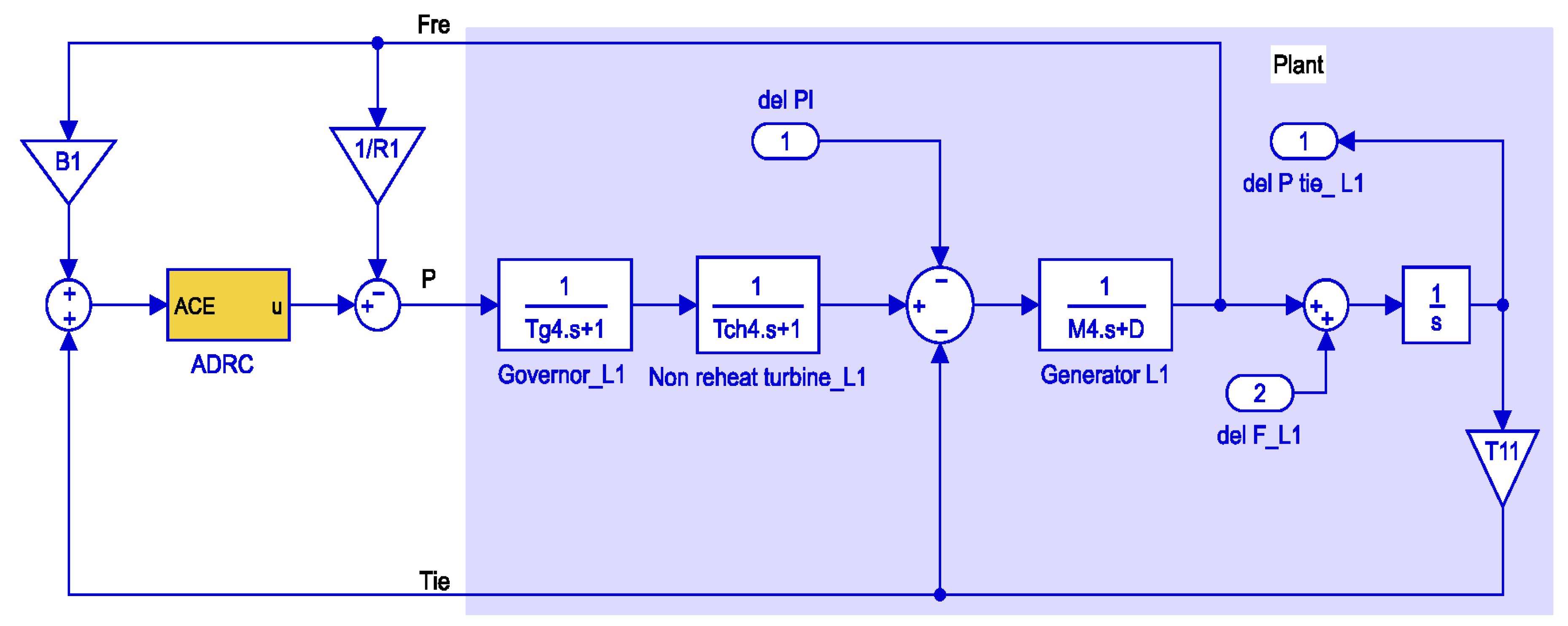
All the power plants (G1, G2 and G3) of Figure 4 are considered similar. The sub-system of power plant 1 is shown in Figure 6. In generation rich areas, a re-heat turbine is used with the governor and generator. The output of the generator of this block is a frequency deviation which is first integrated then multiplied by tie-line synchronizing coefficient between load (L1) to generation (G1) to get the tie-line deviation (del P tie).
The details of a load rich area is shown in Figure 6, where a non re-heat turbine is used with the governor and generator. Finally, considering all these Figure 5, Figure 6 and Figure 7, the complete model of an interconnected power system for ADRC-based LFC is ready to calculate the effect of ACE, frequency deviation and tie-line flow deviation if there is any load change.
3. Factors Influencing ADRC-Based LFC
In an interconnected power system, a lot of parameters may influence the performance of ADRC-based LFC. Nevertheless, some factors that directly dominate the control performance of LFC are discussed in the following sections.
3.1. Tie-Line Synchronizing Coefficient
The total real power that goes out of a particular control area i, , equals to the sum of all outflowing line powers, Ptie,ij in the lines connecting area i with neighboring areas, i.e.,
The simulations are applied to all lines j that terminate in area i. If the line losses are neglected, the individual line power can be written as:
where xij is the reactance of tie-line connecting areas i and j, Vi and Vj are the bus voltages of the line.
If the phase angles deviate from their normal values respectively, one gets the incremental power over the line as given by:
Also:
The phase angles are related to the area frequency changes by:
From the above equations we get:
where:
The Tij is called the tie-line power coefficient or synchronizing coefficient (T).
3.2. Generator Electrical Proximity to the Point of Impact
A power system is generally subject to stochastic power impacts during normal operation due to load changing events. Each of the power impacts is responded to by groups of machines as a form of power swing with different times. The amount of machines’ impacts during faults depends on the distance between the location of the disturbance and the generator and it is termed as generator electrical proximity to the point of impact. In large interconnected power systems, it is very important to investigate how much load impact is being shared by which machine according to their position relative to the disturbance center because the electric power out of a generator may increase or decrease partially depending on the electrical proximity of the generator.
For analyzing the influence of stochastic small load changes at some points in the power system, it is considered that the load has a negligible reactive component as a random change in load creates an imbalance between generation and loadin [32], the mathematical explanations of machine electrical proximity to the point of impact on an interconnected power system are addressed by Equations (16) and (17).The passive electrical network described in [32] has ‘n’ nodes with active sources and i and j nodes are considered two different nodes within the network. The impact of is applied to the new node k. Assuming the network response to be fast the immediate effect of the application of is that the angle of bus k is changed while the magnitude of its voltage k is unchanged. So Pk∆ can be written as:
and are the change in power of nodes i and k at t = 0+ respectively. Psik and Psjk is the change in electrical power of machines i and j respectively due to the change in loads of node k. Equations (13) and (14) show the synchronizing power coefficients of the generators have great influence to share the load impact PL∆ at a network bus k. For this reason, the machine which is located electrically proximity to the point of impact can pick up the highest share of loads regardless of its rating.
3.3. Inertia Constant of Generator
The inertia constant (H) of generator is the ratio of stored kinetic energy in mega joules at synchronous speed with the machine rating in MVA. The effect of H-constant of generator is very important in LFC of an interconnected system, because the higher inertia constant of a generator demonstrates the higher capacity of generator to store the kinetic energy. The mathematical representations of the effect of generator H-constant are presented below from [32].The linearized swing equation for machine i (ignoring damping) is:
The incremental differential equation governing the motion of machine i is given by:
If is constant for all t, the acceleration in p.u. can be computed by using Equation (15):
where is the electrical reference velocity in rad/sec., is the speed of rotor of generator in rad/sec. and is the rated mechanical angular velocity of the shaft in rad/sec.
The p.u. deceleration of machine ith given by Equation (20) is dependent on the synchronizing power coefficient Psik and the Hi constant. The mean acceleration of all the machines in the system can be calculated as:
The individual machine is retarding at various rates while the system as a whole is retarding at a rate provided by Equation (18). Every machine has an oscillatory motion that is operated by its swing equation. When the transient decays, will be the same as as given by Equation (19). Substituting this value of in Equation (13) at t = t1>to:
Thus, after a brief transient period the machines will share increased load as a function of only their inertia constants. These three factors-tie-line synchronizing coefficient, generator electrical proximity to the point of impact and inertia constant of generator have significant impacts on LFC of an interconnected power system which are discussed in Section 4. Finally, an improved ADRC-based LFC model is proposed by introducing new gain in the dynamic model of interconnected power system of Figure 5, Figure 6 and Figure 7.
4. Simulation Results
4.1. Effect of Generator Electrical Proximity to the Point of Impact
4.1.1. Without the Proposed Controller
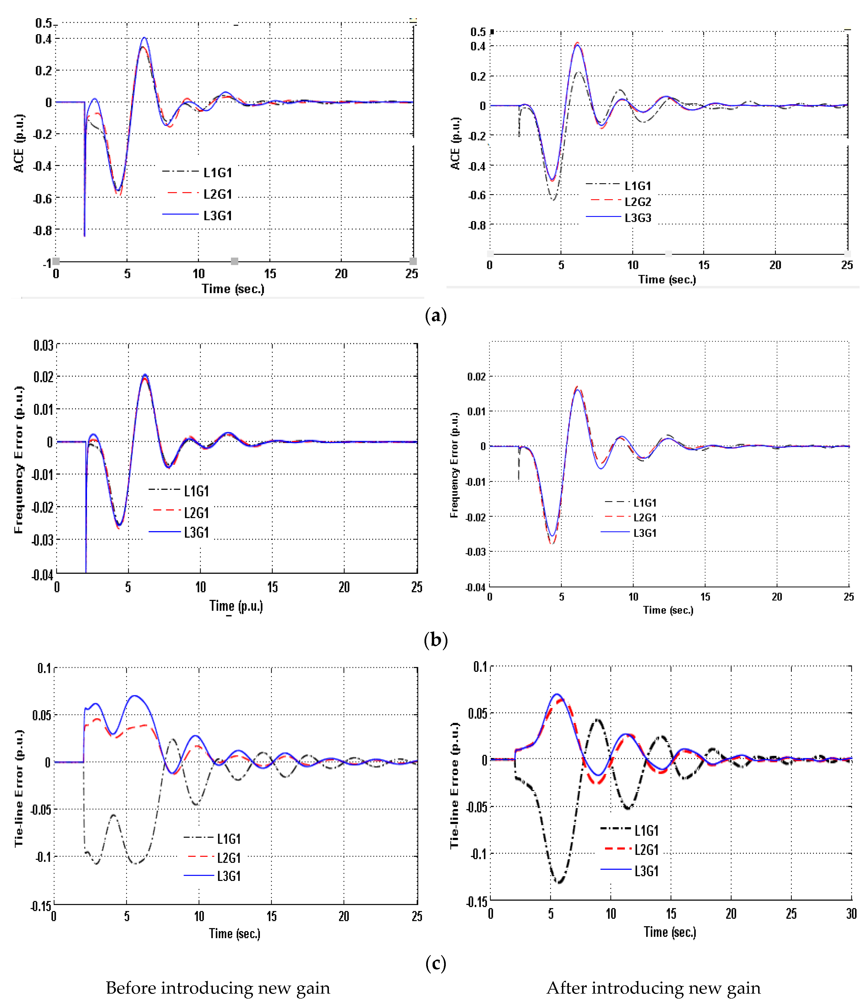
The effect of generator electrical proximity to the point of impact is observed with the ADRC based LFC by applying a load change as disturbance (0.4 p.u.) to the generation rich area (G1) from all load rich areas (L1, L2 and L3) of Figure 5. The distance between two areas (G1 to L1) is represented by the corresponding tie-line synchronizing coefficient (T). A higher value of T decreases the distance between two areas. The values of T are listed in Appendix A, Table A4, and these values are considered only for this specific study. The peak amplitude of ACE, frequency error and tie-line power flow error is considered as the output response in case of ADRC-based LFC. The responses are depicted in Figure 8. Since the load impact is feedback to G1, the output of LFC is taken from G1. The L1G1 indicates the load change is applied from L1 to G1. It is observed that the influence of load changes shared immediately by the generators according to their synchronizing power coefficients. Finally, disturbances are canceled by ADRC and errors become zero.
For the application of the same amount of disturbance from various distances to G1, the response of G1 is shown in Figure 8. It is observed that the magnitude of response is varied according to the distance between G and L. The magnitude of frequency error due to load change from all load canters is noticed as same in Figure 8b and it is because of applying the same amount of load change. However, the tie-line power flows of all cases in Figure 8c are not same because the location of the disturbance from G is not same. So the generators of the system respond according to the electrical proximity to the point of impact as indicated in Equations (16) and (17).
4.1.2. With Proposed Controller
It is desired that the disturbance nearer to the generator will accomplish the greatest response and rest of the generators will show smaller responses. It can be achieved by introducing a new gain block in the dynamic model of the interconnected power system shown in Figure 9.
Tie-line power exchange of a power system is inversely proportional to the transmission line reactance [34]. Besides, the reactance of the transmission lines is a function with the line length. In Figure 10, it is seen that the value of gain is varied with the variation of T and at a certain value of T; the value of gain become fixed. That means after a certain distance the value of gain will be unity as if there is no gain effect on T. This gain parameter will facilitate the generator which is nearest to the disturbance to respond faster. As a result, generators situated at predetermine distance from the point of impact will show their response according to Equations (16) and (17). However, the generators nearer to the point of impact will pick up most of the disturbances.
The effects of generator electrical proximity to the point of impact before and after introducing new gain in ADRC based LFC model of an interconnected power system are revealed in Figure 10 where the same amount of disturbance is applied. A comparison study is presented after and before introducing the new gain block on effect of generator electrical proximity to the point of impact in Table 1. Only the error magnitude ACE (p.u.) is considered for comparison.
It can be seen from Table 1 that G1 is sharing the strongest impact for the application of load change from the L1. On the other hand, due to the load change from L2 and L3, a little influence of disturbance is observed. The time required for settling down the tie-line power flow error is observed longer after introducing new gain in Figure 8c. However, the magnitudes of ACE become lower after introducing the new gain block in Figure 8a. It is observed that ACE in L1G1 is increased after introducing gain because L1 is nearest to G1. ACE increase of any generator means this generator is carrying greater disturbances. So it can be concluded that the generators nearer to the disturbance of an interconnected power system will show the largest response and rest of the generators will show a smaller response.
The proposed new gain is introduced in the dynamic model of power system shown in Figure 9. The value of proposed gain, a, is calculated using Equation (23), where T is the value of tie-line synchronizing coefficient. Figure 10 shows graphically the relationship between the tie-line synchronizing coefficient (T) and the new introduced gain (a).
a = 1−e−2T
4.2. Effect of H-Constant of Generator
4.2.1. Without Proposed Controller
The effect of H-constant of generator on LFC is studied by applying a load change of 0.1 p.u. at t = 2 s by considering the different values of H-constant in the dynamic model of interconnected power system in Figure 5. The output of LFC as ACE, frequency error and tie-line error is presented in Figure 11 after the application of disturbance.
It is observed that minimum ACE belongs to the generator that has larger inertia constant (H = 7) and highest error magnitude belong to the generator which has lowest inertia constant (H = 3) in Figure 11a. The magnitude of frequency error for all cases is examined almost same due to the same amount of load change applied. The oscillation of tie-line power flow error is observed highest for the inertia constant (H = 3) and lowest for (H = 5) in Figure 11c because the generator’s having higher inertia constant are capable of continuing the stable operation during the disturbance.
4.2.2. With Proposed Controller
It is desired that a generator with higher inertia constant should respond more during the disturbance. As a result, the interconnected power system will be able to carry more disturbances without any blackout. To achieve this, it is necessary to add an extra gain block to the dynamic model of the interconnected power system shown in Figure 5. The value of this extra gain block can be determined by normalizing the H-constant of existing generators. The average value of three generator’s H-constant is 5, so normalized value is considered as 5. The value of new gain block is calculated by dividing the generator’s H-constant by 5. The process of selecting the value the value of new gain block is presented in Table 2.
The effect of H-constants in LFC of an interconnected power system after introducing new gain is represented in Figure 11 by applying the same amount of disturbance.
In Figure 11a, the responses of all generators are almost same and the magnitudes become lesser after applying the normalized gain parameters. So, all the generators are showing same responses regardless of their H-parameters and time required to settle down the responses become lesser in Figure 11.
Figure 12 illustrates how the new gain block is introduced in the dynamic model of interconnected system.
5. Comparison among ADRC-Based LFC
A comparison among the standard ADRC, ADRC considering tie-line synchronizing co-efficient (T), and ADRC considering generator H-constant for an ADRC-based LFC is tabulated in Table 3. Load change of 0.1 p.u. is applied separately from L1, L2 and L3.
The magnitude of ACE represents the generator response. The higher magnitude of ACE of generator belongs to higher response due to load change. It can be seen from the second column of Table 3 that due to the same amount of disturbance, the response of L1G1 becomes the highest since G1 is considered nearest to the disturbance. In the third row, due to the new introduced gain with T consideration, the error magnitude (ACE) of L1G1 has increased from 0.60 p.u. to 0.83 p.u. On the other hand, the error magnitudes are decreased in L1G2 and L1G3, so the nearest generator is carrying the highest disturbance impact.
In the fourth row, the H-constant of generators are considered as 3, 5 and 7 for G1, G2 and G3 respectively, so due to the application of disturbance, the response of G1 become highest where it is lowest in G3, but if all the generators of an interconnected power system respond equally during the disturbance, then the generator’s with higher H constant will share the higher load change impact. This is achieved by introducing the new gain shown in the fifth row. Therefore, it can be concluded that it is a fast acting ADRC-based LFC. Comparing the proposed ADRC controller and standard ADRC controller, the simulation results reveal that the proposed controller can provided an improved performance for LFC during random and continuous load disturbances.
6. Conclusions
This paper proposes a new ADRC-based LFC model in a complicated interconnected power system to improve the transient responses of frequency error of power plant and diminish the magnitude error of ACE. A proportional factor is introduced in the system, which assist in reducing magnitude error and suppress transient errors. It is observed that synchronous machines, which are electrically closer to the point of impact, pick up the greatest share of the load regardless of their size, whereas other machines do not need to respond. Besides, the inertia constant (H) of generator has an effect on system frequency response. Response of generator with higher inertia constant is increased, while response is decreased for generators of lower inertia constant. As a result, power system will be able to continue its operation with less abnormality. The proposed ADRC-based LFC controller is found to demonstrate a better and faster response characteristic compared to standard controllers. Furthermore, the proposed controller is capable of sustaining the interconnected system during disturbances.
Author Contributions
Md Mijanur Rahman and A Hasib Chowdhury built and calibrated the simulation model described in the paper and participated in the proposal and analysis of the solutions. Md Alamgir Hossain has enriched the manuscript in terms of scientific and technical expertise with improving the paper quality. All authors contributed to bringing the manuscript in its current state.
Conflicts of Interest
The authors declare no conflict of interest.
Appendix A

Table A1.
System parameters for Figure 5.
Table A1.
System parameters for Figure 5.
| Parameters | Definition | Value |
|---|---|---|
| Tch (sec.) | Turbine time constant | 0.3 |
| R (Hz/p.u.) | Speed regulation coefficient | 0.05 |
| Fhp (p.u.) | High pressure stage rating | 0.3 |
| M (p.u.sec.) | Area inertia constant | 10 |
| D (p.u./Hz) | Area load damping constant | 1.0 |
| Tg (sec.) | Governor time constant | 0.2 |
Table A2.
ADRC parameters.
| Parameters | Non-Reheat Turbine Unit | Reheat Turbine Unit |
|---|---|---|
| Order of ESO | 3 | 4 |
| 4 | 4 | |
| 16 | 20 | |
| b | 70.0 | 70.0 |
Table A3.
Value of tie-line synchronizing coefficient for Figure 5.
Table A3.
Value of tie-line synchronizing coefficient for Figure 5.
| Tie-line Synchronizing Coefficient | Value | Tie-Line Synchronizing Coefficient | Value |
|---|---|---|---|
| T11 | 25 | T32 | 25 |
| T21 | 30 | T13 | 20 |
| T31 | 40 | T23 | 35 |
| T12 | 30 | T33 | 30 |
| T22 | 24 |
Table A4.
Nomenclature.
| Mi | Area Inertia Constant | Di | Area Load Damping Constant |
| Tchi | Turbine time constant | Tgi | Governor time constant |
| Ri | Speed regulation coefficient | B | Area frequency response characteristic |
| Fhp | High pressure stage rating | Trh | low pressure reheat time |
References
- Tomsovic, K.; Bakken, D.E.; Venkatasubramanian, V.; Bose, A. Designing the Next Generation of Real-time Control, Communication, and Computations for Large Power Systems. Proc. IEEE 2005, 93, 965–979. [Google Scholar] [CrossRef]
- Kundur, P. Power System Stability and Control; McGraw-Hill: New York, NY, USA, 1994. [Google Scholar]
- Moon, Y.; Ryu, H.; Lee, J.; Kim, S. Power System Load Frequency Control Using Noise-Tolerable PID Feedback. In Proceedings of the IEEE International Symposium on Industrial Electronics, Pusan, Korea, 12–16 June 2001; Volume 3, pp. 1714–1718. [Google Scholar]
- Kothari, M.; Sinha, N.; Rafi, M. Automatic Generation Control of an Interconnected Power System under Deregulated Environment. In Proceedings of the Power Quality’98 Conference, Hyderabad, India, 18 June 1998; Volume 18, pp. 95–102. [Google Scholar]
- Ikhe, A.; Kulkarni, A. Load Frequency Control for Interconnected Power System Using Different Controllers. Autom. Control Intell. Syst. 2013, 1, 85–89. [Google Scholar] [CrossRef]
- Roy, L.; Dey, B. Load Frequency Control in Interconnected Power System by Using Classical Controller. Int. J. Electron. Comput. Sci. Eng. 2015, 3, 22–25. [Google Scholar]
- Panda, G.; Panda, S.; Ardil, C. Automatic Generation Control of Interconnected Power system with Generation Rate Constraints by Hybrid Neuro Fuzzy Approach. Int. J. Electr. Power Energy Syst. Eng. 2009, 2, 13–18. [Google Scholar]
- Han, J. From PID to Active Disturbance Rejection Control. IEEE Trans. Ind. Electron. 2009, 56, 900–906. [Google Scholar] [CrossRef]
- Kumar, I.P.; Kothari, D.P. Recent Philosophies of Automatic Generation Control Strategies in Power Systems. IEEE Trans. Power Syst. 2005, 20, 346–357. [Google Scholar]
- Hiyama, T.; Koga, S.; Yoshimuta, Y. Fuzzy Logic Based Multi-Functional Load Frequency Control. In Proceedings of the IEEE Power Engineering Society 2000 Winter Meeting, Singapore, 23–27 January 2000; Volume 2, pp. 921–926. [Google Scholar]
- Yukita, K.; Goto, Y.; Mizuno, K.; Miyafuji, T.; Ichiyanagi, K.; Mizutani, Y. Study of Load Frequency Control Using Fuzzy Theory by Combined Cycle Power Plant. In Proceedings of the IEEE Power Engineering Society 2000 Winter Meeting, Singapore, 23–27 January 2000; Volume 1, pp. 422–427. [Google Scholar]
- Mohamed, H.A.F.; Hassan, L.H.; Moghawemi, M.; Yang, S.S. Load Frequency Controller Design for Iraqi National Super Grid System Using Fuzzy Logic Controller. In Proceedings of the SICE Annual Conference, Tokyo, Japan, 20–22 August 2008; pp. 227–232. [Google Scholar]
- Inoue, S.; Ishida, Y. Design of a Model-following Controller Using a Decoupling Active Disturbance Rejection Control Method. J. Electr. Electron. Syst. 2016, 5, 174. [Google Scholar] [CrossRef]
- Rerkpreedapong, D.; Hasanovic, A.; Feliachi, A. Robust Load Frequency Control Using Genetic Algorithms and Linear Matrix Inequalities. IEEE Trans. Power Syst. 2003, 18, 855–861. [Google Scholar] [CrossRef]
- Chi, R.; Liu, Y.; Hou, Z.; Jin, S. Data-Driven Terminal Iterative Learning Control with High-Order Learning Law for a Class of Non-Linear Discrete-Time Multiple-Input–Multiple Output Systems. IET Control Theory Appl. 2015, 9, 1075–1082. [Google Scholar] [CrossRef]
- Precup, R.-E.; Radac, M.-B.; Roman, R.-C.; Petriu, E.M. Model-Free Sliding Mode Control of Nonlinear Systems: Algorithms and Experiments. Inf. Sci. 2017, 381, 176–192. [Google Scholar] [CrossRef]
- Xiao, Y.; Hong, Y.; Chen, X.; Huo, W. Switching Control of Wind Turbine Sub-Controllers Based on an Active Disturbance Rejection Technique. Energies 2016, 9, 793. [Google Scholar] [CrossRef]
- Gao, Z.; Huang, Y.; Han, J. An Alternative Paradigm for Control System Design. In Proceedings of the IEEE Conference on Decision and Control, Orlando, FL, USA, 4–7 December 2001; Volume 5, pp. 4578–4585. [Google Scholar]
- Gao, Z. Scaling and Bandwidth-Parameterization Based Controller Tuning. In Proceedings of the American Control Conference, Denver, CO, USA, 4–6 June 2003; pp. 4989–4996. [Google Scholar]
- Gao, Z. Active Disturbance Rejection Control: A paradigm Shift in Feedback Control System Design. In Proceedings of the American Control Conference, Minneapolis, MN, USA, 14–16 June 2006; pp. 16–18. [Google Scholar]
- Qi, X.; Bai, Y. Improved Linear Active Disturbance Rejection Control for Microgrid Frequency Regulation. Energies 2017, 10, 1047. [Google Scholar] [CrossRef]
- Movva, K.; Reddy, Y.V.L.C. Automatic Generation Control of Multi-Area Power System Using Active Disturbance Rejection Control. Int. J. Eng. Trends Technol. 2017, 43, 236. [Google Scholar]
- Zhang, Y. Load Frequency Control of Multiple-Area Power Systems. Master’s Thesis, Cleveland State University, Cleveland, OH, USA, August 2009. [Google Scholar]
- Miklosovic, R.; Gao, Z. A Robust Two-Degree-of-Freedom Control Design Technique and Its Practical Application. In Proceedings of the IEEE Industry Applications Conference, Clearwater, FL, USA, 2–6 May 2004; Volume 3. [Google Scholar]
- Sayem, A.H.M. Active Disturbance Rejection Control for Load Frequency Control of Bangladesh Power System. Master’s Thesis, Bangladesh University of Engineering and Technology, Dhaka, Bangladesh, November 2012. [Google Scholar]
- Liu, N.; Fei, J. Active Disturbance Rejection Control of Active Power Filter. In Proceedings of the 2016 19th International Conference on Electrical Machines and Systems (ICEMS), Chiba, Japan, 13–16 November 2016. [Google Scholar]
- Zhang, Y.; Dong, L. On Design of a Robust Load Frequency Controller for Interconnected Power System. In Proceedings of the American Control Conference, Baltimore, MD, USA, 30 June–2 July 2010. [Google Scholar]
- Sayem, A.H.M.; Cao, Z.; Man, Z. Performance Enhancement of ADRC Using RC for Load Frequency Control of Power System. In Proceedings of the 2013 IEEE 8th Conference on Industrial Electronics and Applications (ICIEA), Melbourne, Australia, 19–21 June 2013. [Google Scholar]
- Yang, J.; Zeng, Z.; Tang, Y.; Yan, J.; He, H.; Wu, Y. Load Frequency Control in Isolated Micro-Grids with Electrical Vehicles Based on Multivariable Generalized Predictive Theory. Energies 2015, 8, 2145–2164. [Google Scholar] [CrossRef]
- Liu, N.; Lyu, X.; Zhu, Y.; Fei, J. Active Disturbance Rejections Control for Current Compensation of Active Power Filter. Int. J. Innov. Comput. Inf. Control 2016, 12, 407–418. [Google Scholar]
- Shanmuga, V.; Jatabarathi, T. A Novel Approach of Load Frequency Control in Multi Area Power System. Int. J. Eng. Sci. Technol. 2011, 3, 2494. [Google Scholar]
- Anderson, P.M.; Fouad, A.A. Power System Control and Stability, 2nd ed.; IEEE Press: Piscataway, NJ, USA, 2002. [Google Scholar]
- Parniani, M.; Nasri, A. SCADA Based under Frequency Load-Shedding Integrated with Rate of Frequency Decline. In Proceedings of the 2006 IEEE Power Engineering Society General Meeting, Montreal, QC, Canada, 18–22 June 2006. [Google Scholar]
- VijayaChandrakala, K.R.M.; Balamurugan, S.; Sankaranarayanan, K. Damping of Tie-Line Power Oscillation in Interconnected Power System Using Variable Structure System and Unified Power Flow Controller. J. Electr. Syst. 2012, 8, 85–94. [Google Scholar]
Figure 1.
Architecture of ADRC.
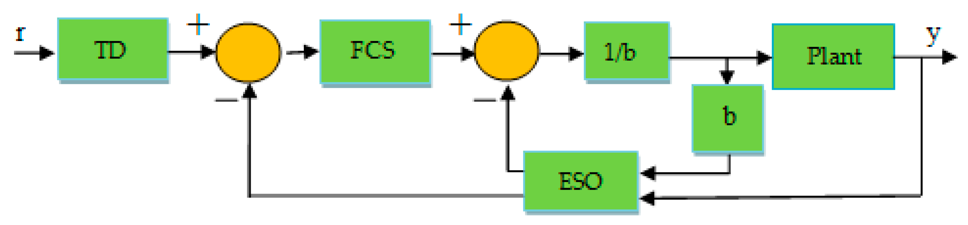
Figure 2.
Block diagram of ADRC-based LFC.
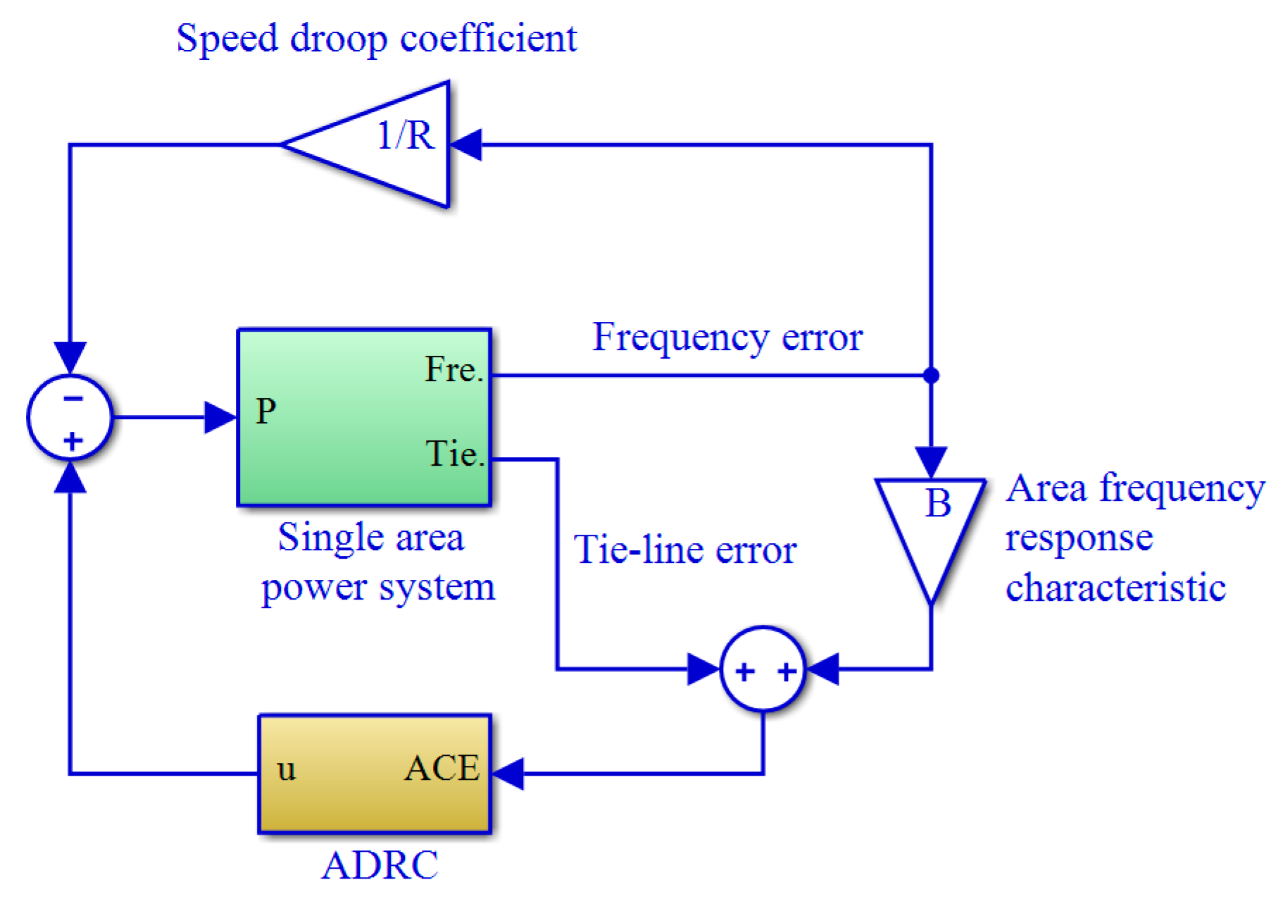
Figure 3.
Proposed ADRC-based LFC model for generator electrical proximity to the point of impact.
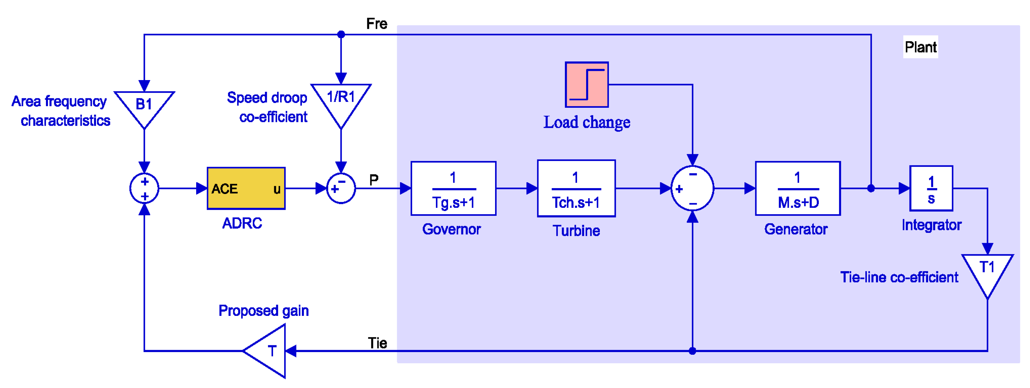
Figure 4.
Proposed ADRC-based LFC model for generator H-constant effect.
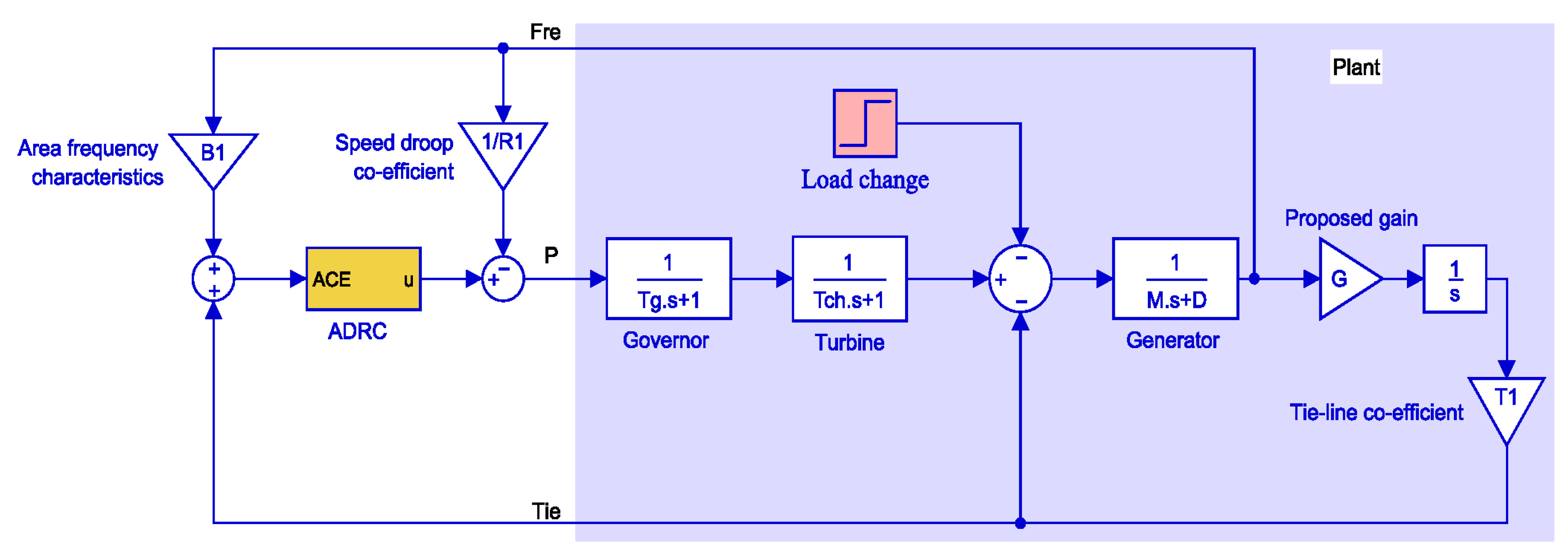
Figure 5.
Dynamic model of interconnected power system for ADRC-based LFC.
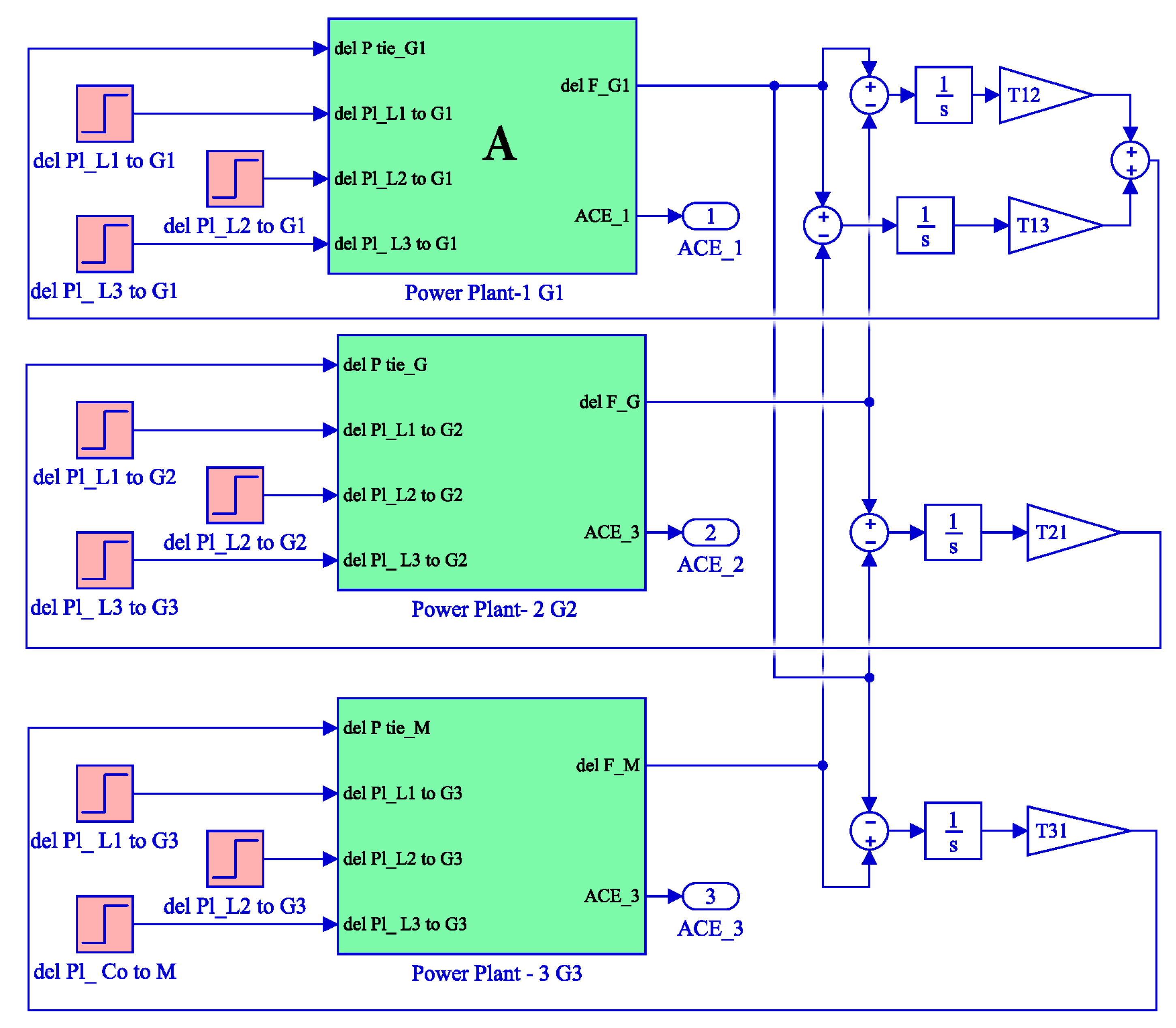
Figure 6.
Dynamic model of power plant 1 (block A in Figure 5).
Figure 6.
Dynamic model of power plant 1 (block A in Figure 5).
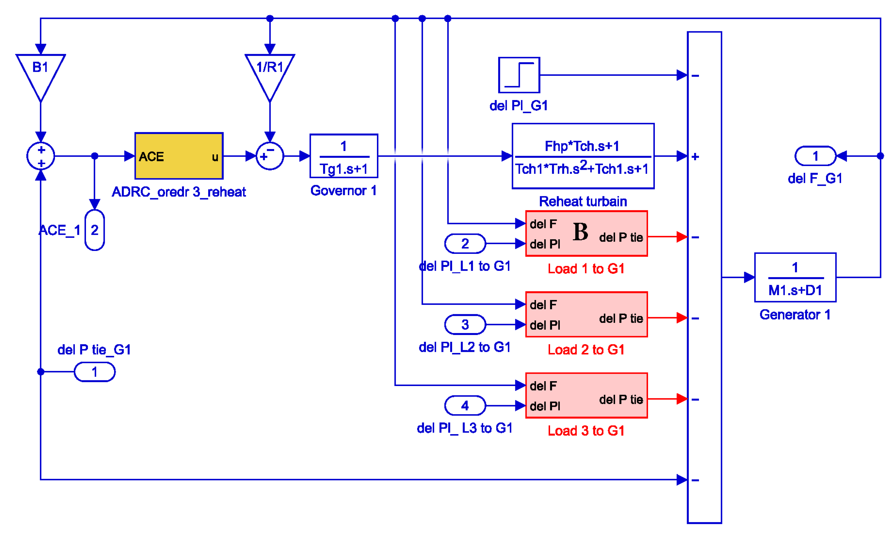
Figure 7.
Dynamic model of load change from L1 to G1 (block B in Figure 6).
Figure 7.
Dynamic model of load change from L1 to G1 (block B in Figure 6).

Figure 8.
Effect of generator electrical proximity to the point of impact on generator G1 before and after introducing new gain on: (a) ACE, (b) frequency error, and (c) tie-line error.
Figure 8.
Effect of generator electrical proximity to the point of impact on generator G1 before and after introducing new gain on: (a) ACE, (b) frequency error, and (c) tie-line error.

Figure 9.
Proposed dynamic model for load change from L1 to G1.
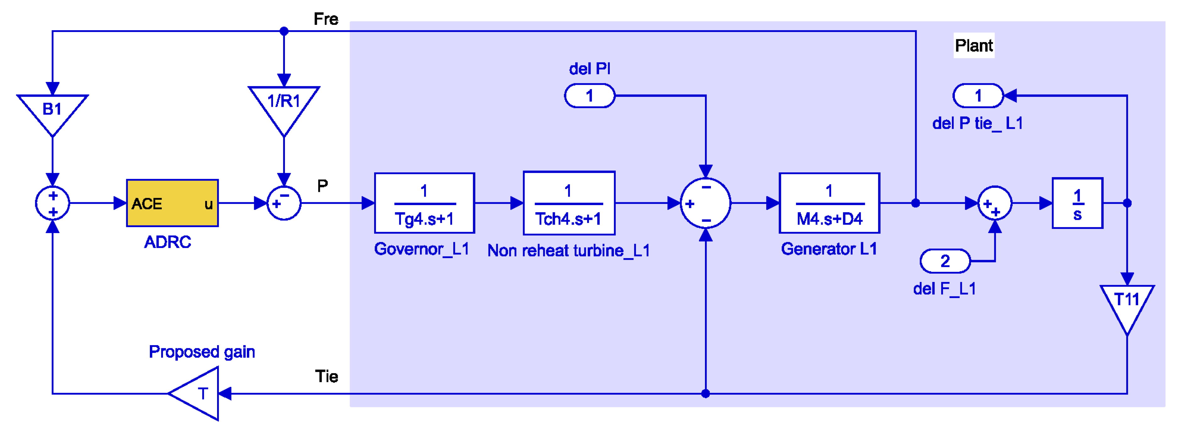
Figure 10.
Relation between tie-line synchronizing coefficient (T) and new introduced gain (a).
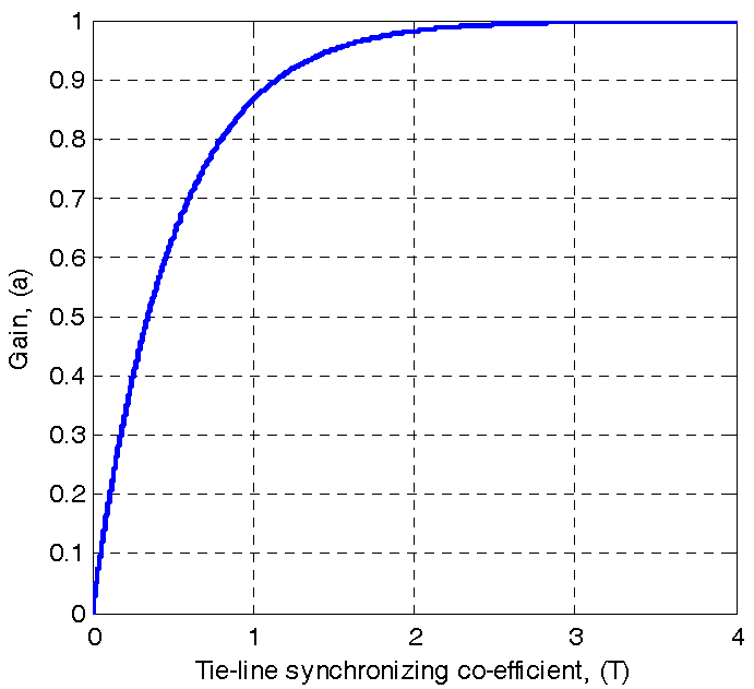
Figure 11.
Effect of H-parameter on: (a) ACE, (b) frequency error, and (c) tie-line error before and after introducing an extra gain block.
Figure 11.
Effect of H-parameter on: (a) ACE, (b) frequency error, and (c) tie-line error before and after introducing an extra gain block.
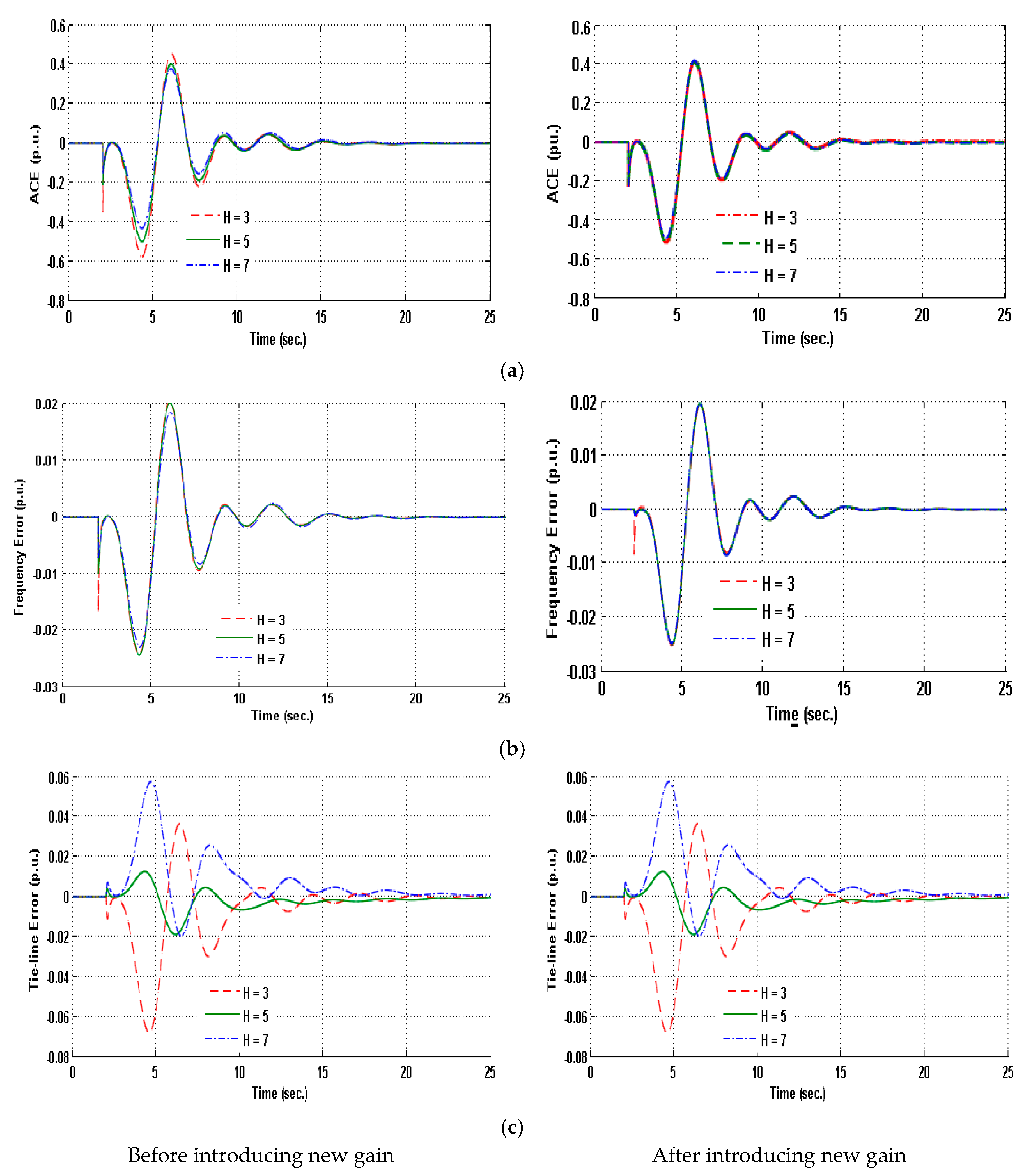
Figure 12.
Proposed dynamic model of power plant 1.
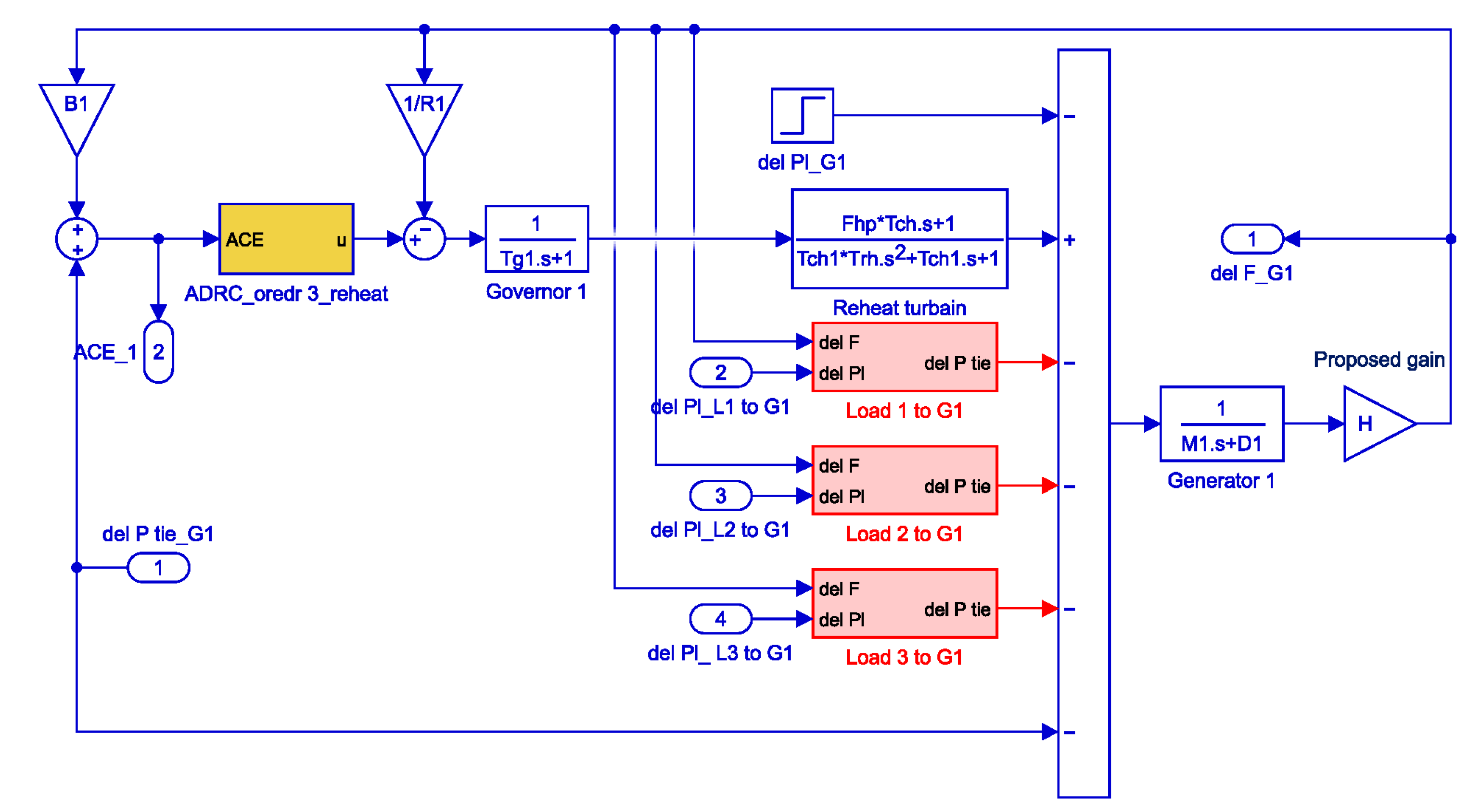
Table 1.
Comparison of the effect of electrical proximity introduced through a gain block on ACE for different feedback connection.
Table 1.
Comparison of the effect of electrical proximity introduced through a gain block on ACE for different feedback connection.
| Feedback Connection | Tie-Line Synchronizing Coefficient (T) | ACE (p.u.) | |
|---|---|---|---|
| Without New Gain Block | With New Gain Block | ||
| L1G1 | 80 | 0.59 | 0.65 |
| L2G1 | 25 | 0.55 | 0.53 |
| L3G1 | 50 | 0.56 | 0.53 |
Table 2.
Normalizing system of H-constant.
| Value of H-Constant | Normalized Value | Value of New Gain |
|---|---|---|
| 3 | 5 | 3/5 |
| 5 | 1 | |
| 7 | 7/5 |
Table 3.
Comparison among standard ADRC, ADRC with T and ADRC with H constant for ADRC based LFC with different feedback connection.
Table 3.
Comparison among standard ADRC, ADRC with T and ADRC with H constant for ADRC based LFC with different feedback connection.
| Sl. No. | ADRC Type | ACE (p.u.) for Different Feedback Connections | ||
|---|---|---|---|---|
| L1G1 | L1G2 | L1G3 | ||
| 1 | Standard ADRC | 0.58 | 0.57 | 0.55 |
| 2 | ADRC with T consideration | 0.60 | 0.54 | 0.525 |
| 3 | ADRC with T and new introduced gain consideration | 0.83 | 0.50 | 0.45 |
| 4 | ADRC with H constant consideration | 0.575 | 0.50 | 0.43 |
| 5 | ADRC with H constant and new introduced gain consideration | 0.52 | 0.52 | 0.51 |
© 2017 by the authors. Licensee MDPI, Basel, Switzerland. This article is an open access article distributed under the terms and conditions of the Creative Commons Attribution (CC BY) license (http://creativecommons.org/licenses/by/4.0/).
Share and Cite
MDPI and ACS Style
Rahman, M.M.; Chowdhury, A.H.; Hossain, M.A. Improved Load Frequency Control Using a Fast Acting Active Disturbance Rejection Controller. Energies 2017, 10, 1718. https://doi.org/10.3390/en10111718
AMA Style
Rahman MM, Chowdhury AH, Hossain MA. Improved Load Frequency Control Using a Fast Acting Active Disturbance Rejection Controller. Energies. 2017; 10(11):1718. https://doi.org/10.3390/en10111718
Chicago/Turabian StyleRahman, Md Mijanur, A. Hasib Chowdhury, and Md Alamgir Hossain. 2017. "Improved Load Frequency Control Using a Fast Acting Active Disturbance Rejection Controller" Energies 10, no. 11: 1718. https://doi.org/10.3390/en10111718
Note that from the first issue of 2016, this journal uses article numbers instead of page numbers. See further details here.