Optimal and Learning-Based Demand Response Mechanism for Electric Water Heater System


1
Department of Electrical and Computer Engineering, The University of Alabama, Tuscaloosa, AL 35487, USA
2
Department of Computer Science, The University of Alabama, Tuscaloosa, AL 35487, USA
*
Author to whom correspondence should be addressed.
Energies 2017, 10(11), 1722; https://doi.org/10.3390/en10111722
Submission received: 16 September 2017
/
Revised: 6 October 2017
/
Accepted: 24 October 2017
/
Published: 27 October 2017
(This article belongs to the Section F: Electrical Engineering)
Abstract
:This paper investigates how to develop a learning-based demand response approach for electric water heater in a smart home that can minimize the energy cost of the water heater while meeting the comfort requirements of energy consumers. First, a learning-based, data-driven model of an electric water heater is developed by using a nonlinear autoregressive network with external input (NARX) using neural network. The model is updated daily so that it can more accurately capture the actual thermal dynamic characteristics of the water heater especially in real-life conditions. Then, an optimization problem, based on the NARX water heater model, is formulated to optimize energy management of the water heater in a day-ahead, dynamic electricity price framework. A genetic algorithm is proposed in order to solve the optimization problem more efficiently. MATLAB (R2016a) is used to evaluate the proposed learning-based demand response approach through a computational experiment strategy. The proposed approach is compared with conventional method for operation of an electric water heater. Cost saving and benefits of the proposed water heater energy management strategy are explored.
1. Introduction
Electricity consumption in residential markets will undergo fundamental changes in the next decade due to the emergence of smart appliances and home automation. A key requirement for the smart appliances within the smart grid framework is the demand response (DR). DR is defined as changes in electricity usage by end-use customers from their normal consumption patterns in response to changes in the price of electricity (price-responsive DR), or to incentive payments designed to induce lower electricity use at time of high wholesale market prices or when system reliability is jeopardized (curtailable DR) [1]. This paper focuses on price-responsive DRs.
A primary component for a successful price-responsive DR program is an intelligent home automation system (HAS). Basically, a HAS receives information about weather forecast, dynamic electricity pricing, device operating characteristics, usage requests, etc. and autonomously makes control decisions and sends control actions to smart appliances. The task of the HAS is to produce an optimal solution for a weighted combination of objectives and determine a series of control actions to take over time to manage the operation or energy consumption of all home appliances.
According to [2], the top electricity consumptions in US homes are heating, ventilation and air conditioning (HVAC), electric stoves, water heating, refrigeration, lighting, dryer, dishwasher, computers and television. Among these appliances, HVAC, water heating, dishwasher and dryer are primary DR capable appliances. Significant research efforts have been focusing on developing demand response and energy management for HVAC [3,4]. Particularly, Zhang et al. [3] developed a learning-based HVAC energy management system mechanism that can identify and update energy consumption model daily for an HVAC to determine an optimal DR policy, which makes the DR management of HVAC adaptive to seasons, users and house condition changes and therefore more efficient. However, except for HVACs, learning-based DR researches on other DR capable appliances and are limited.
Electric water heater (EWH) is one of the commonly-used appliances in a house and is also a major DR capable appliance. According to [5], it accounts for 7.5% to 40% of total domestic energy usage. When comes to the mechanism of EWH, there are some similarities between HVACs and EWHs. By controlling the power input, both systems can provide different temperature output for the need of consumers. In addition, they have similar thermodynamic equations. However, there are several obvious differences between a HVAC and an EWH system. First, EWH must meet the minimum temperature tolerance of a customer; otherwise, the customer might get cold water during shower which is unacceptable compared to the comfort impact due to control error in a HVAC system. Second, conventional water heaters have a water tank which can be considered as a thermal energy storage unit. Therefore, optimal energy management can be applied to an EWH in a similar way as the energy management in electric vehicles and solar PV systems [6]. Third, equivalent hot water stored in a water tank must be managed properly. Otherwise, there will not be sufficient hot water available to meet customer demand.
For energy optimization and demand response using EWHs, Du et al. [7] proposed an approach of solving the EWH commitment problem instead of solving the optimization problem through a two-step scheduling process, in which the EWH model is based on an estimated EWH thermal model. In [8], the authors used an on/off model to determine the operation of an EWH, which would certainly make results obtained different from the actual EWH behavior especially for those new EWHs having adjustable operational capability. In addition, the water demand or customer comfort factor was not integrated with the optimization of EWH operation, and the optimization problem was focusing on balancing wind power generation with energy consumption of multiple EWHs. Xu et al. [9] presented a detailed study on the partial differential equation (PDE) physics-based model of an EWH. However, unlike a data driven or learning based model, the model presented in [9] cannot reflect EWH model variations caused by external conditions and over time. Belov et al. [10] used a fixed EWH thermal model and a two-stage optimization process to determine the operation of an EWH in a double-price tariff framework between day and night, in which the energy-comfort and expense-comfort issues are considered. In [11], the same approach of [10] was used to determine the optimal operation of multiple EWHs in a demand response framework.
In general, in all the above works, the EWH model is typically fixed instead of adaptive over time; water demand forecast, a critical factor to determine EWH demand response, is not properly considered in the EWH optimization problem formulations; the relationship between the water temperature of EWH tank and the warm water demand actually needed by users is not addressed; and the operation of the EWH is based on a simplified on/off mechanism. All these factors are properly considered and addressed in this paper. The paper develops learning-based adaptive algorithms to learn EWH energy consumption model and customer behavior on hot water demand to enhance energy management technique of an EWH system in a DR framework under different seasons, weather, and user conditions. The learning-based algorithms are integrated into the EWH optimization problem and the supply–consume relation between the temperatures of hot water in EWH tank and warm water needed by consumers is properly considered. Therefore, the special features of the paper include:
- A mechanism to develop a data driven NARX (nonlinear autoregressive network with external input) model for a typical electric water heater through learning the “measured” data, and the EWH model is updated daily through learning with new data.
- A prediction method to estimate customer water demand behavior on the household electric water heater, by which the customer’s hot water volume consumption is collected, updated, and learned daily.
- An EWH supply–consume model to compute equivalent warm water that can be used by users when the average water temperature in EWH tank is either higher or lower than the demanded water temperature needed by users.
- A genetic algorithm to determine the optimal energy management of EWH to minimize the energy consumption cost. The optimization is obtained based on learned customer’s hot water usage pattern, learned thermal dynamic model of EWH system, and day-ahead electricity price.
In the sections that follow, the paper first analyzes conventional water heater model and control methods as well as how to build them into an EWH simulation system using MATLAB Simulink in Section 2. In addition, Section 2 presents how to obtain a data-driven EWH model by training artificial neural networks based on target data generated from the EWH simulation for a typical household. In Section 3, a hot water supply–consume model is proposed to determine the maximum capability of the EWH. Section 4 presents a genetic algorithm based optimization algorithm that can minimize the EWH energy consumption cost while maintaining the comfort of customers. Section 5 gives the simulation results and comparison study based on MATLAB. The simulation combines different environmental conditions with EWH neural network model, hot water demand prediction model and dynamic electricity prices for DR development and evaluation. Section 6 concludes the paper.
2. Electric Water Heater Modeling
2.1. Basic Structure of Water Heater
A water heater typically uses gas or electricity to heat the water and to meet the demand of the household occupants. Most residential water heaters in North America have traditionally been the tank-type water heater. It consists of a cylindrical vessel or container that keeps water warm or hot to make the water be ready to use by occupants at any time. Typical sizes of residential water heaters can hold water ranging from 20 to 100 gallons. These water heaters may consume energy from electricity, natural gas, propane, heating oil, solar, or other energy sources. This paper focuses on electric water heaters, one of the most popular water heaters used in a common U.S. household.
The water tank of an EWH usually has one pipe on the bottom of the tank used to pump cold water into the tank and one pipe on the top of the tank used to lead hot water out from the tank as shown in Figure 1a. There are commonly one or two heating elements inside the tank. A tanked EWH has the advantage of using electricity at a relatively slow rate compared to a tankless water heater because it can store the hot water in the tank for later use. The disadvantage is that, to keep the water hot in the tank and be ready to use at any time, the heating system of the EWH has to be turned on occasionally.
For a tanked EWH with conventional control, the water is maintained at a constant temperature setting point due to the lack of knowledge of customer water usage behavior and comfort preference. Figure 1b illustrates traditional EWH on–off control method. In general, when water tank temperature reaches an upper limit, the heater turns off; when it reaches a lower bound, the heater turns on. According to [4], the average heating time of a household EWH is around 2.6 h per day. Since the conventional EWH cannot recognize high and low price hours, there is a large room for improvement in control optimization. In addition, without optimization, the tank size must be large enough, because undersize tank may not meet the comfort requirement of a customer at peak usage hour.
2.2. Thermodynamic Model of Water Heater
The thermal dynamic model of an EWH was traditionally derived based on system energy balancing relation as shown in [7]. Basically, power enters an EWH and heats the heating elements and water in the tank; hot water flows out of the tank for the customer to use. In addition, thermal energy losses due to imperfect thermal insulation make up a part of the power consumption. Hence, the mathematical model of the EWH thermal system [12] can be represented as:
where M (kg) is the mass of water in the tank, c (J/kg °C) is the specific heat of water, (kg) is the mass flow rate, h is the heat transfer coefficient for convection to the ambient, A (m2) is the area of heat transfer which is the surface area of water tank, Ttank (°C) is the average temperature of the tank as water in tank is considered as ideally homogeneous; Tinput (°C) is the temperature of the input cold water, Tamb (°C) is the temperature of the environment, and Q(t) (W) is the heating element power.
2.3. Simulink Model of Electric Water Heater
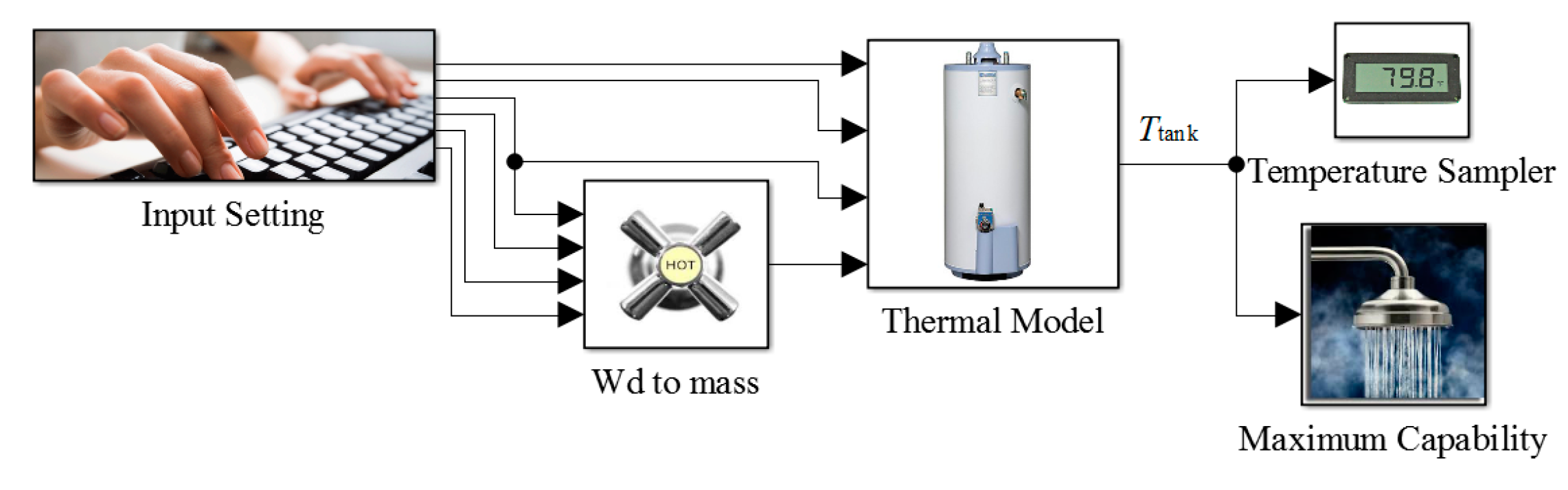
An overall EWH system, based on Equation (1), was implemented using MATLAB Simulink, as shown in Figure 2. The input settings of the system go to the thermal model as well as to the unit conversion block. The thermodynamic model is implanted in the thermal model. It calculates tank temperature based on electric power input, input cold water temperature, environment temperature, and mass flow rate. The maximum capability block calculates the maximum hot water volume ready to be used based on several input settings and tank temperature obtained from EWH Thermal block. Then, temperature of the EWH can be obtained by running the simulation model for 24 h. By default, the initial EWH temperature is set as 10 °C (50 °F). All parameters are first converted to the International System (SI) of units before being applied to the EWH simulation model.
Energy consumption of an actual EWH is much more complicated because the parameters associated with the EWH model could be largely deviate from manufacturer’s specified values and EWH heat transfer mechanism is more complicated than that represented in Equation (1). In addition, the power efficiency of the water heater could change over time due to aging problems and change in environment conditions. As a result, developing a learning mechanism that can update the EWH model on schedule and adapt changes in the parameters is critical for the optimal energy management of an EWH.
2.4. Generating Training Data
As mentioned above in Section 2.2, the output temperature of an EWH tank at hour n, , depends on the previous tank temperature , current power input Qn, water demand Wdn, input cold water temperature and ambient temperature . Based on this analysis, the EWH model with its inputs and outputs can be represented by:
where the training target data for an adaptive EWH model was generated through the model shown in Figure 2. By providing random input power Q within the rated power limit of 4500 W, Wd, and to the model, with a simulation time step of 1 s and simulation length for 24 h, the output target temperature data are generated and collected.
Since the electricity price and weather forecast obtained from electric utility company and U.S. national weather service were broadcasted in hours, in this paper, we divided each day into 24 time slots, i.e., one hour for each time slot. Hence, the proposed EWH model needs to be represented or generated based on hours, which means that all the input and output data of the EWH model should be represented in terms of hours. Therefore, after getting the raw data from the EWH simulation model shown in Section 2.2, the data need to be processed into hourly data. The temperature data are converted into hourly mean, EWH power input is converted into hourly mean, and the water demand in each hour is the summation of total water demand in that hour. Table 1 shows a set of processed hourly data obtained from the MATLAB EWH simulation model.
2.5. Learning NARX EWH Model
Several methods have been applied in the modeling of residential HVACs and EWHs. Besides the PDE model presented in [9], a third-order polynomial linear regression function to build a data driven model for an HVAC system was proposed in [7]. However, the linear regression method only performs a best fitting line or a best fitting plane, which could result in a considerable error when applied to EWH with highly nonlinear characteristics. In [13], an artificial neural network for predicting domestic hot water characteristics is presented. However, it has a relatively high error rate. To overcome the challenge, a NARX model using neural network is proposed to learn the actual EWH model.
NARX is a recurrent dynamic network, with feedback connections enclosing several layers of the network. We implement the NARX model by using a feedforward neural network to approximate the model. Using NARX, we can predict time series output given past values of the same time series and the feedback input.
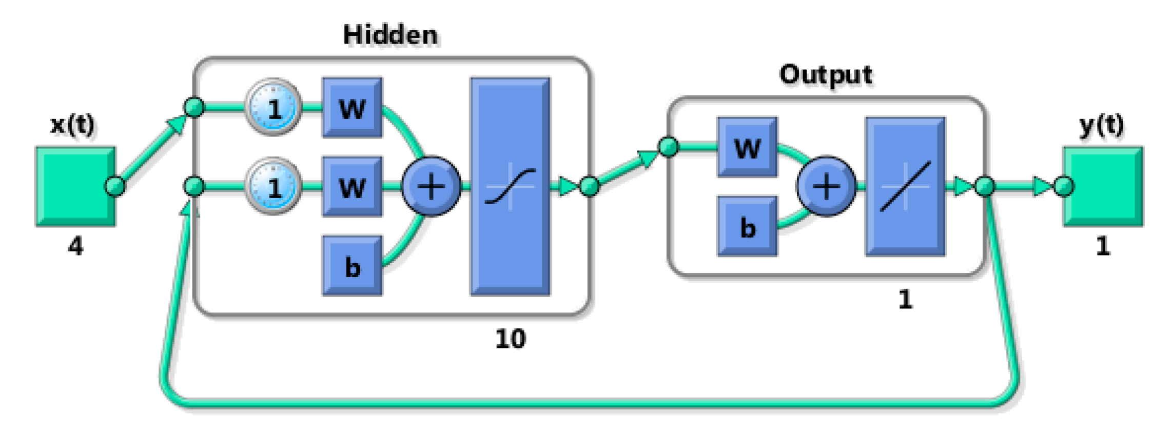
We used a three-layer network to learn the EWH model, which consists of an input layer, a hidden layer, one output layer, and one feedback connection from the output of the network to the input of the network. The input layer consists of five inputs represented by X shown in Equation (2), which also includes the feedback input. The hidden layer has 10 neurons. The output layer gives or predicts the water temperature of the tank at the next time slot. In this paper, a Levenberg–Marquardt method was used as the training method to train the network. The NARX structure of the network generated by using MATLAB Neural Network toolbox is shown by Figure 3.
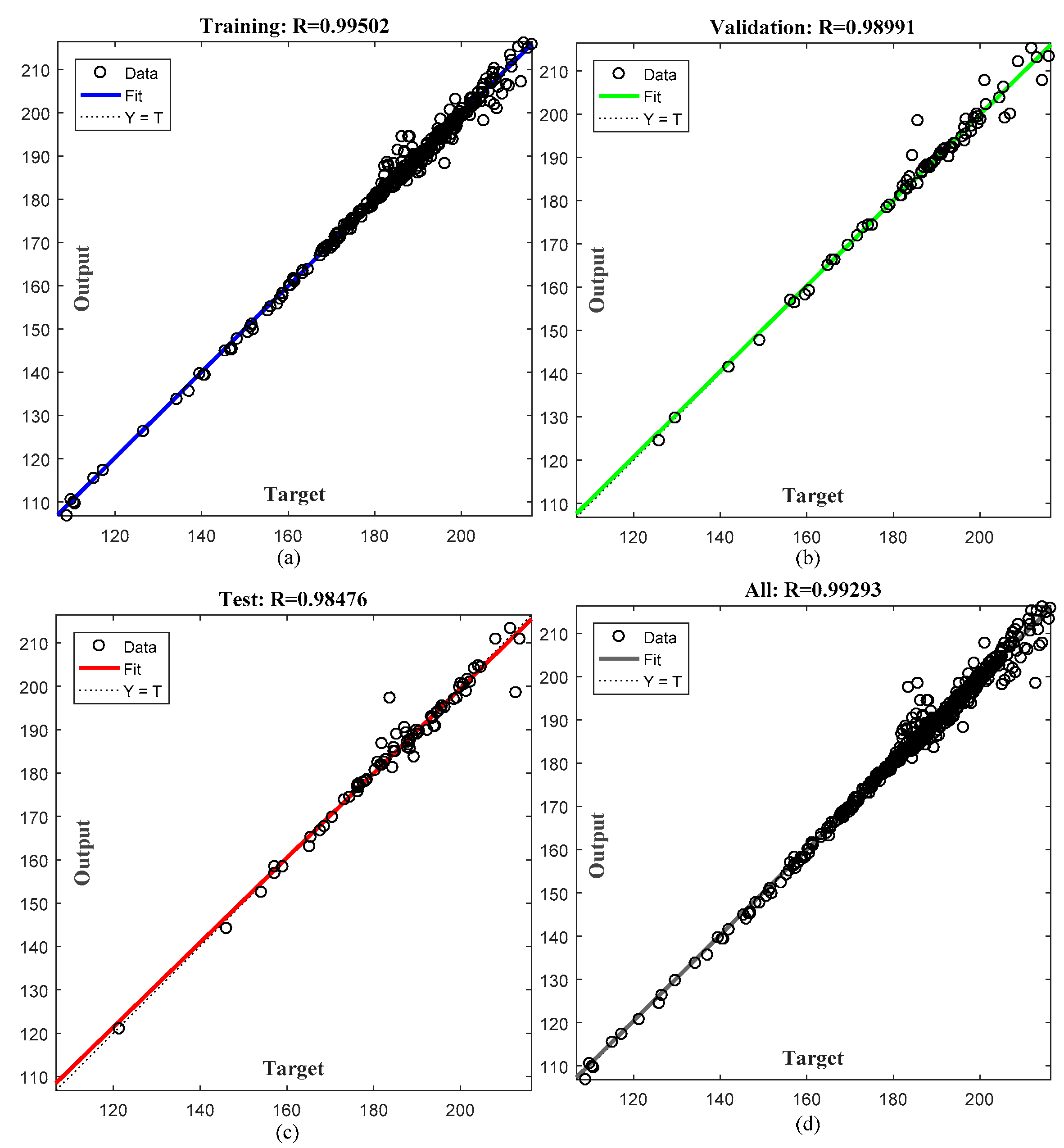
The processed data for a period of one week are divided into training, validation and testing datasets with proportions of 70%, 15% and 15%, respectively. The NARX training performance evaluation is shown in Figure 4, which contains four subfigures for performance evaluation corresponding to training, validation, testing and overall datasets. Each subfigure shows in the output-target plane: (1) the neural network output and target data pairs; (2) line regression of the output and target data relationship; (3) a line of Y (output) = T (target); and (4) an R value for measuring the goodness-of-fit. For the best training effect, the regressed line should overlap with the Y = T line and R value should be 1. As shown in Figure 4, the network was well trained.
After the training, we can obtain a NARX neural network function with input and output . Note that the network training is updated every day with new data to make the trained network able to capture the EWH energy consumption properties under different seasons, weathers and household conditions. By using NARX (•) function, EWH water temperature can be predicted recursively as:
3. Hot Water Supply–Consume Model
In this paper, a new way of modeling the supply of hot water is proposed. We proposed the virtual concept of maximum hot water capability Wmax (gallon) to represent the maximum hot water volume the water heater can provide. Wmax is a function of Ttank, Q and Tbase in which Tbase is the lowest temperature consumers can accept as usable hot water, and is a variable due to seasonal changes. The whole tank of water is regarded as hot water when Ttank is above Tbase; otherwise, it is regarded as not usable cold water.
The Wmax we proposed in the Supply–Consume model is a virtual water volume; instead of showing the real hot water volume inside the tank, it take into account the total volume of hot water in the coming hour. If Wmax is larger than Wd, it means the scheduled Q is a valid power consumption solution, which meets the customer demand. This constraint of Wmax larger than Wd will be used in later optimization constraint sets in Equation (8). In addition to Wmax, we proposed a term called equivalent hot water Weq (gallon) to represent the actual hot water consumers can use given Ttank because, when water from hot-water faucet is too hot, consumers normally mix it with cold-water faucet water to get a moderate temperature.
Therefore, if Ttank is below Tbase, the equivalent hot water volume Weq is zero since nothing is usable; if Ttank is above Tbase, Weq would be larger than tank volume. It will consist of hot water stored in the tank mixed with the cold water from the cold-water faucet. The hotter the water in the tank, the larger the equivalent hot water volume Weq will be. Take 110 °F as the base temperature and 50 °F as the cold-water faucet temperature for example, an adjustable coefficient (Ttank − 50)/60 should be applied to obtain the equivalent hot water volume Weq shown as:
The equation is developed based on specific heat formula and the first law of thermodynamics. In Equation (4), Ke is the efficiency of the tank heat preservation and it is usually set as 0.7 due to heat dissipation.
In addition to Weq, Wmax also includes Re which is the part of water heated up by heating elements. It is calculated based on empirical Equation (5) provided by EWH company shown in [14].
where is the temperature difference between and Tbase. δ is an empirical constant that equals 2.442. The volume of the water tank Vtank in this paper is sized as 50 gallons or 0.189271 m3, a typical residential EWH tank size. The maximum heating element power rating is set as 4500 W. In [8], the relationship between different water heater tank sizes and power rating was discussed among different households. This paper will focus only on optimal energy management of EWH.
As mentioned above, if Ttank is lower than Tbase, Wmax only depends on the newly heated water since the water in tank is not usable. In addition, since Equation (5) is an empirical formula, it does not consider the situation that Ttank is very close to Tbase; hence, we build a regression model replacing the recovery rate formula in order to avoid invalid results.
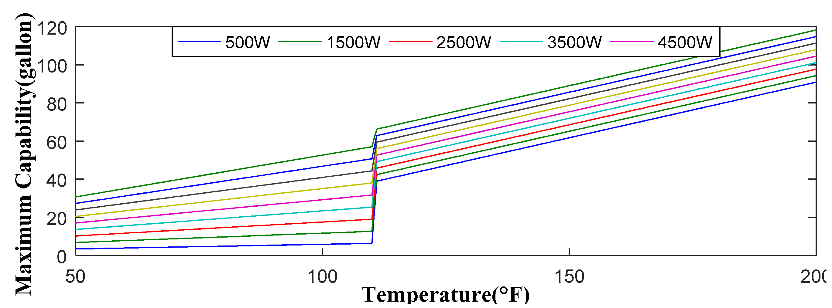
Thus, considering the above factors, Wmax can be calculated using Equations (6)–(8). The maximum capability we can have given different tank temperature and input power with Tbase equal to 110 °F is shown in Figure 5.
We proposed Algorithm 1 to integrate Equations (4)–(8). By using Algorithm 1, we can get the maximum capability Wmax of each hour and use it as one of the constraints later in Section 4.3. In Algorithm 1, we have tank temperature Ttank in advance by using Equation (3).
| Algorithm 1: Calculating Maximum Capability of EWH | |
| 1: | at the previous day |
| 2: | for n = 1 to 24 do |
| 3: | |
| 4: | if |
| 5: | |
| 6: | else |
| 7: | |
| 8: | end if |
| 9: | end for |
4. Optimizing EWH Power Input under Demand Response Framework
The demand pattern of customer is an important reference in EWH energy management. If we can accurately predict the demand pattern in advance, it is then possible to arrange demand side management (DSM) in designed time slots [6]; the EWH can work on schedule and can save considerable amount of energy.
4.1. Forecasting the Customer’s Demand Pattern
For different houses, the demand pattern is always unique [8,15]. Even in the same household, in different seasons such as summer and winter, the demand pattern is also different. Because of this unique feature, it is necessary to develop a prediction mechanism for each individual household.
Several methods have been proposed to forecast the customer’s demand pattern using the history consumption data of the customers. In [16], a Bayesian updating approach is applied to learn the probability of customer hot water usage behavior at each hour, in which a large data set is needed to learn the model before using it. Other methods, including seasonal naïve and seasonal decomposition in conjunction with exponential smoothing (STL and ETS), were discussed in [17]. However, when initially starting the DSM for an appliance, the forecast process starts with very limited historical data available for modeling. Hence, using the above methods will lead to considerable error.
In addition, the residential hot water consumption pattern has a lot of uncertainty due to stochastic events such as guest visiting, vacations, etc., thus many studies affirmed the inability to model and predict domestic hot water consumption [18,19,20]. To overcome these challenges, [17,20] used models that have multi-function prediction. Inspired by these models, this paper uses a time series decomposition forecasting methods, seasonal autoregressive integrated moving average (ARIMA) to forecast customer water demand pattern. The seasonal ARIMA (p,d,q) (P,D,Q)m model is a well-established modeling technique that combines autoregressive (AR) part, moving average (MA) part and integrated (I) part of a prediction progress where parameters p, d, and q are non-negative integers representing the order of the AR model, degree of difference and the order of the MA model. Comparatively, parameters P, D, and Q are seasonal AR, MA and I parts of the model. In addition, m refers to the number of periods in each season. Figure 6 shows the performance of five forecasting methods given the real public load forecasting data from Global Energy Forecasting Competition 2014 (GEFCom2014). It includes Seasonal mean method, MA method, ARIMA (3,1,1) with seasonal MA, ARIMA (1,1,1) (1,0,2)24 and ARIMA (1,1,2) (1,0,0)168. The fourth and fifth methods are chosen from the optimal methods in [17]. The red line is the target load data from GEFCom2014, it has a two peaks in each 24 h interval and also a long term tide. All five forecast methods can follow the two peaks but they all have error to some extent in forecasting the long term load tide. The initial learning week is not shown in the figure.
In this paper, we use the most general practices to evaluate the performance of the forecast methods, including the normalized mean absolute error (nMAE), normalized root mean square error (nRMSE) and mean absolute scaled error (MASE) of different forecast methods as defined in [17,21]. Table 2 summarizes the performance of the above five methods. In Table 2, ARIMA (1,1,2) (1,0,0)168 has the best performance in nMAE and MASE; ARIMA (3,1,1) with SMA24 perform better in nRMSE. Therefore, ARIMA (1,1,2) (1,0,0)168 is chosen as the optimal forecast method in the optimization algorithm latterly used in this paper. To have more accurate forecast model, different climate and economic scenarios [22] should also be put into consideration. Due to limitation of space, further discussion is not included.
4.2. Day-Ahead Price
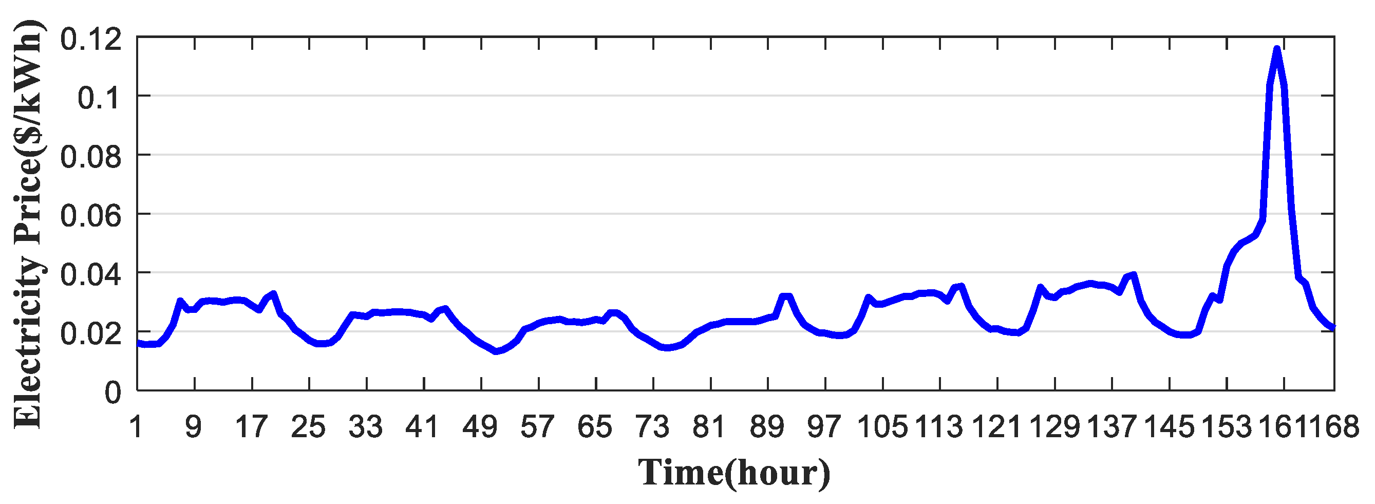
In a flat electricity price market, a customer would use an appliance without the concern of price changing. However, in a price fluctuating market, which is the real situation, customers are encouraged to shift the working hours of appliances because consume electricity with low price will reduce their utility bills. The 24-h electricity price can be provided by an electric utility one day ahead under a dynamic pricing program. The real-time electricity price and day-ahead price of a utility company can be found in [23]; the company serves about 2.4 million customers in Illinois and Missouri. Figure 7 shows the seven-day electricity price posted on their website starting on 1 October 2015.
With the day-ahead price, one can develop power management algorithm for EWH to optimize the cost of the EWH by decreasing energy consumption during higher price hours and increasing energy consumption during lower price hours. This would help to cut down the electricity bill of the customer. In addition, some constraints should be considered to maintain the comfort experience of customer.
4.3. Genetic Algorithm Based Optimization
The optimization of electricity cost has been investigated in [24] for HVAC demand response using particle swarm optimization. For nonlinear models, global search metaheuristic methods are efficient to find near-optimal solutions. In our paper, we chose genetic algorithm (GA) based optimization method to search for input power solution that has the minimum energy cost.
The objective of the GA-based optimization is to minimize the cost of electricity used by EWH. It can be modeled as:
In Equations (9) and (10), Pn and Qn represent day-ahead electricity price and power input of EWH at hour n, respectively. The constraints in Equation (10) are the range of EWH power and the range of EWH capability. is determined by using Algorithm 1. Water tank is similar to other energy storage units but the cost to “charge” and “discharge” is negligible compared to battery and fuel cells, hence there is no constraint put on switch times. The detail of the GA-based algorithm is explained in Algorithm 2.
| Algorithm 2: GA-based EWH optimization | |
| 1: | Population initialization: generating a population of k chromosomes randomly within the power range |
| {Execute GA algorithm} | |
| 2: | for i = 1 to Nlimit do |
| 3: | Calculate using ARIMA (1,1,2) (1,0,0)168 |
| 4: | Calculate using Algorithm 1 |
| {Calculating the fitness of each chromosome} | |
| 5: | for j = 1 to k do |
| 6: | If then |
| 7: | |
| 8: | else |
| 9: | |
| 10: | end if |
| 11: | Call GA Routine according to [25] |
| 12: | end for |
| 13: | end for |
| 14: | Collect the best chromosome, i.e., the best power input solution for the cost function in (9) |
| 15: | Output the best fitness value Fbest, i.e., the minimum cost for operating EWH |
With the above DSM, customers can have the lowest cost spend on EWH while their comfort of using the hot water remains the same.
4.4. Win–Win Situation for System Operator and Customer
From the grid side, to meet all the energy demand from customers, the grid capacity needs to be designed to satisfy the peak power demand. In a typical household, the load will be much higher when customers are active at home. The main consumption time of conventional EWH is during 7:00 a.m.–11:00 a.m. and 6:00 p.m.–12:00 a.m., i.e., when people usually have showers [26]. When performing EWH DSM, it is ideal to shift the EWH load from formal peak hours to valley hours to reduce the peaks. The valley hours corresponds to hours when appliances are idle and residents are usually inactive. The simulation in Section 5 will demonstrate the effect of load shifting.
The peak-to-average power ratio (PAPR) is a measure of the power waveform, showing the ratio of peak values to the average value. That PAPR equals 1 indicates no peak which is the ideally desired goal in terms of DSM. The closer PAPR gets to 1, the less power loss will occur on the grid side. In [27,28], distributed algorithm and game theory are proposed to reduce PAPR in DSM. One of the main reasons that electric prices vary in a day is that, in peak hours when total demand is high, more expensive generation sources are added to meet the increased demand [29]. For the proposed DSM under this pricing strategy, the shifting of EWH demand can reduce the peak hour demand in the grid [30]. The new power consumption solution will have a PAPR much closer to 1 due to the rearranging of the power consumption.
However, for renewable power resources such as wind and solar, the power generation itself already has a large PAPR due to the uncertainty of weather, which would require that a DSM approach should be designed to shift load pattern towards the power generating pattern considering renewables.
5. Simulation Analysis
This section first evaluates the optimal energy solution obtained from the proposed GA-based optimization of EWH energy management. It also evaluates the peak-to-average ratio of the EWH energy schedule and the total energy cost as performance index. All simulations were conducted in MATLAB R2016a environment.
5.1. GA-Based Optimal EWH Energy Management
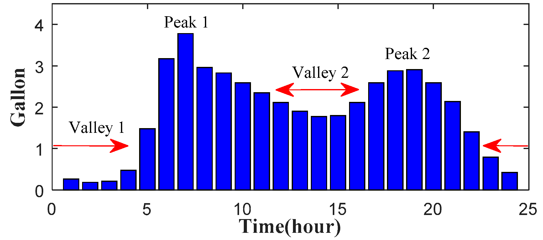
The optimization of EWH energy management is based on water demand pattern recorded in [31]. The 24-h water demand pattern of a typical household is shown in Figure 8. It has two peaks at Hours 7 and 19 and two valleys at Hours 2 and 14. The day-ahead electricity price is based on data from [23].
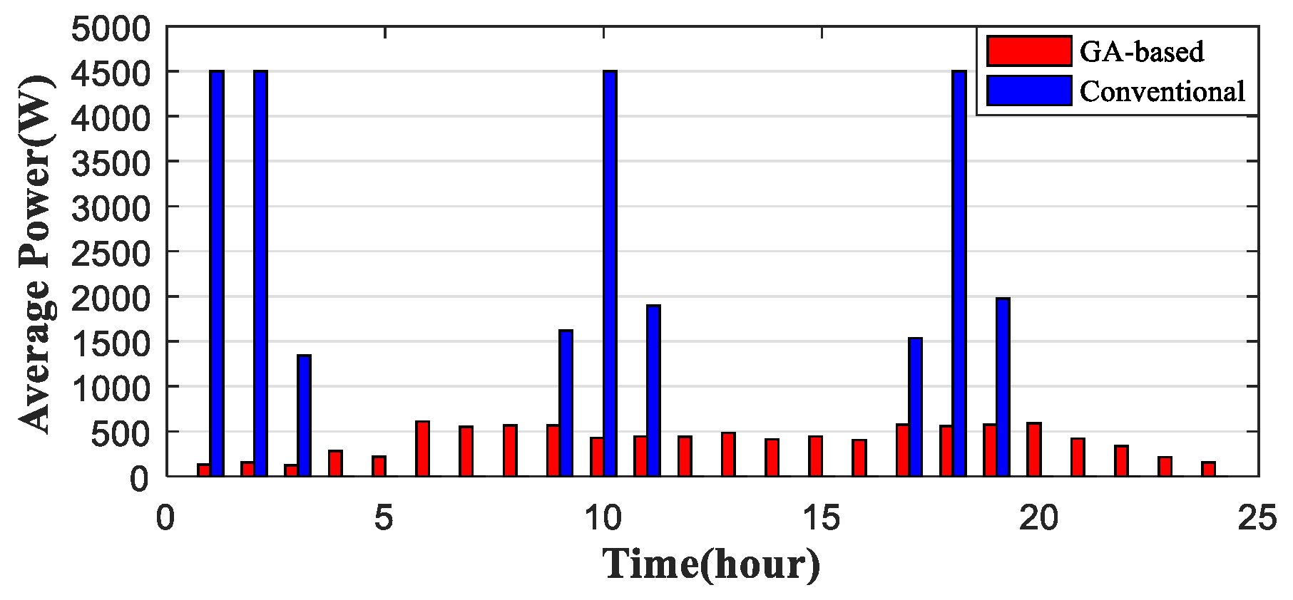
Figure 9 shows the comparison of EWH power consumption solution between GA-based and conventional methods in a 24-h simulation. It is clear that GA-based algorithm reduces the overall EWH load greatly. Due to the demand forecast, the proposed GA-based algorithm scheduled the power consumption solution just to reach the requirement and saved a lot of energy compared with conventional solution. It also shifts some portion of the peak load to the valley hours between Hour 1 and Hour 5 when the electricity price is low. For conventional control regardless of demand and the price, it shows several peak load hours, such as Hours 1, 2, 10 and 18.
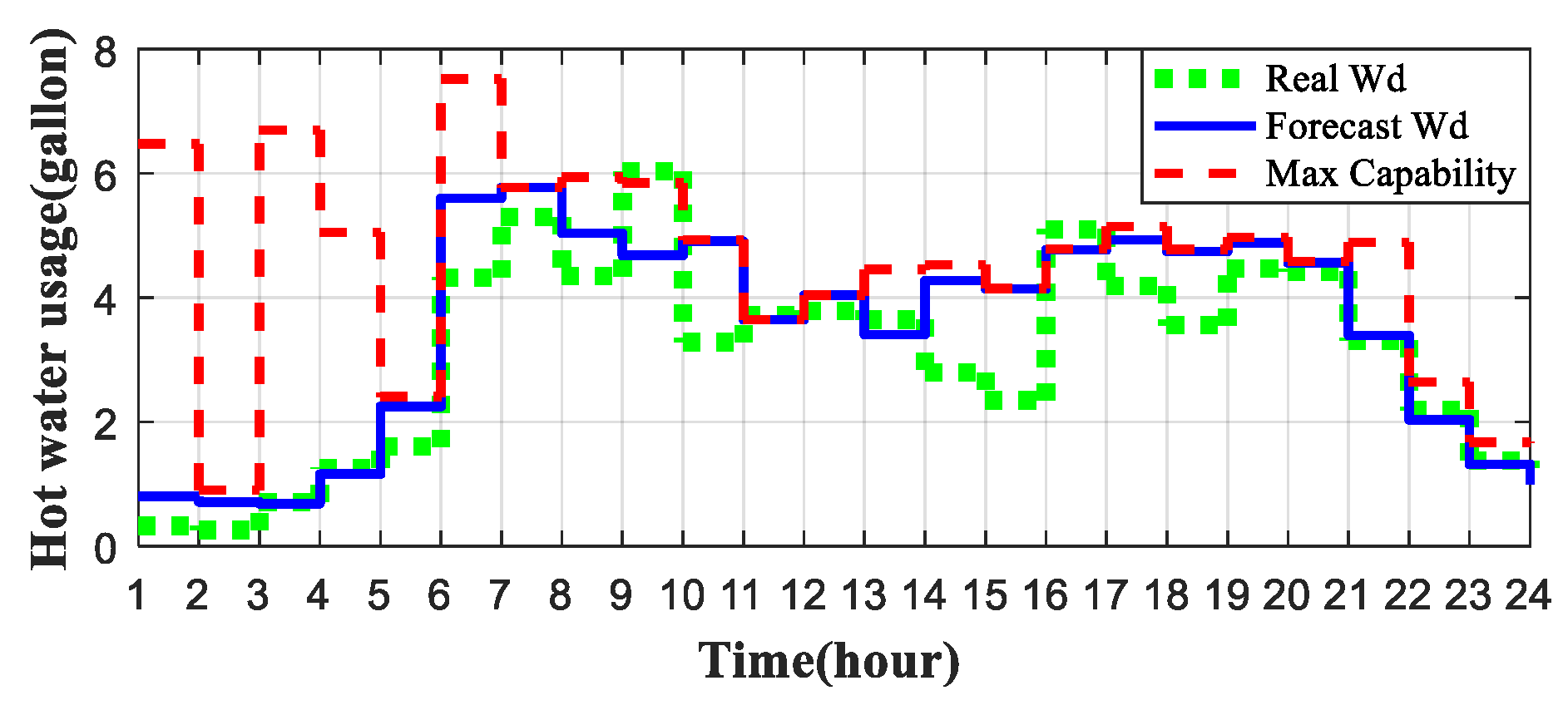
Besides finding the power consumption solution with minimum cost, we would like to make sure that the comfort experience of the customer is not affected, i.e., the maximum capability of the EWH, , can meet the hot water demand of the customer. In Figure 10, the real hot water demand from residents, shown in Figure 8, is redrawn by the green dotted line in this figure; the forecasted hot water demand, generated using the ARIMA model shown in Section 4.1, is shown in the blue line; the red dotted line represents the maximum capability of the hot water that can be provided at a given time slot and is calculated based on the Supply-Consume model presented in Section 3. In Hour 9 and Hour 16, there are, respectively, 0.189 gallon and 0.351 gallon of hot water shortage. This is due to the error in water demand forecast. In these two time slots, the maximum hot water capacity generated using the proposed Supply–Consume model is above the forecasted water demand generated using the ARIMA model, demonstrating the effectiveness of the proposed method in general. However, the maximum hot water capacity is a little bit below the real hot water demand represented by the green dotted line due to the prediction error between the actual and forecasted water demands, indicating that improvement is needed in the water demand forecast. Even so, the prediction and actual water demand patterns are properly matched with each other in Figure 10. Since none of the existing forecast technologies can guarantee 100% forecast accuracy, and also the shortage calculated in Figure 10 is less than 7% of the overall daily hot water usage, it is reasonable to assume that this hot water shortage is negligible. Hence, the solution generated using the proposed method is a valid solution to maintain the overall comfort of customers. Note that the learning and GA-based optimization approach works in a 24-h frame, i.e., there is no consecutive optimization between two consecutive days. As a result, in the late-night hours starting at 10:00 p.m., the power decreases, as there is no further known usage of hot water from the next day.
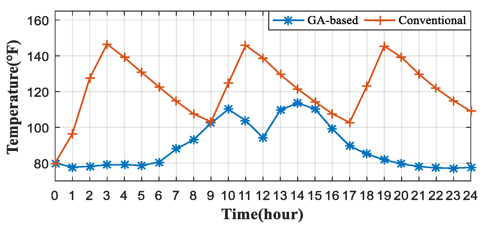
In addition, the comparison of the tank temperature is shown in Figure 11. For GA-based model, the tank temperature is always lower than the conventional one because of the optimized power solution. It rises only according to the demand of the customer and a huge amount of energy can be saved.
It is needed to point out that, even though the electricity cost is minimized, the total energy consumption cannot be guaranteed as minimum. The algorithm tends to schedule more power in lower price hours, whereas heat loss will take place while storing the hot water for later demand.
In [32], a dual-tank water heater is applied to improve this shortcoming. The tanks in the dual-tank system do not have equal volume and can have different maintenance temperature. In this case, another optimization can be applied to decrease surplus output.
5.2. Impact of Proposed Mechanism under Residential Power System
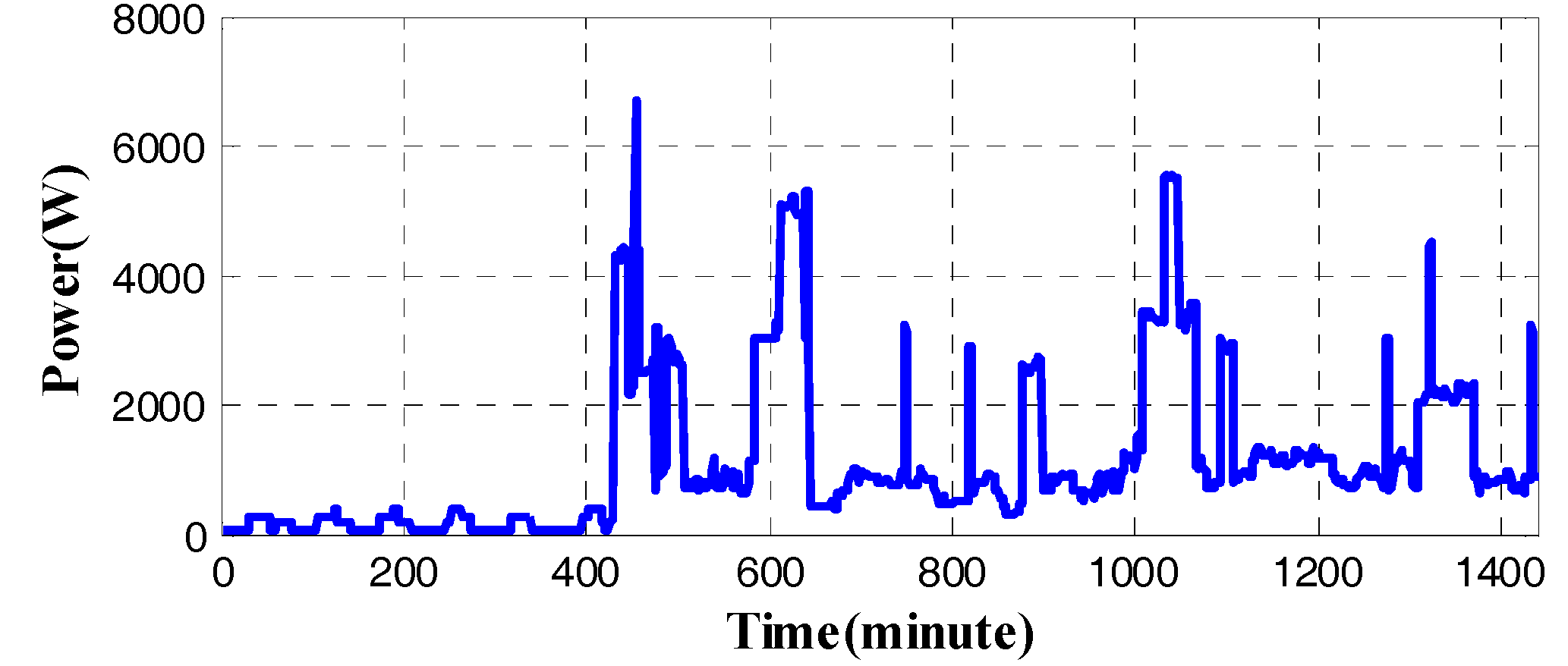
To evaluate the impact of the proposed EWH mechanism to the residential power system, an overall demand load pattern is considered. The residential load pattern is simulated using a domestic electricity demand model provided in [33], and the load of water heater is excluded from the pattern. The demand of a residential house with five residents was simulated for a weekday in October. The load pattern is shown in Figure 12, in which we can see that, without EWH, there are already several peak hours. The results of Figure 12 matches with the discussion presented in Section 4, which shows that, during the active hours of residents, the demand is high while in midnight, the demand is low.
For the conventional EWH power consumption pattern shown in Figure 9, the usage peaks appear at similar peaks, as shown in Figure 12, since the EWH usage also happens in the active hours of residents. However, the peak hours of the GA-based EWH solution are shifted to the non-peak hours of other appliances. This is demonstrated by Figure 13, which shows the overall load pattern including EWH. In Figure 13, the solid black line is the total load pattern without EWH which is the same as that shown in Figure 12. By adding the conventional and GA-based power consumption patterns shown in Figure 9 to the black line, respectively, the overall residential load patterns are shown by the green dotted line and blue dotted line in Figure 13. In the load pattern using the conventional EWH method (green dotted line), the load peak is added with the other load peak in Hours 10 and 17–19, while, in GA-based load pattern (blue dotted line), the peak reduces.
The comparison of PAPR and weekly cost using conventional and GA-based EWH is shown in Figure 14. The conventional EWH has a PAPR of 3.89. The GA-based EWH has a PAPR reduced to 2.86. For comparison, the PAPR without EWH load is also shown in Figure 14, which is 3.72. PAPR is largely reduced after the learning and GA-based optimization compared to the DSM result using a Vickrey-Clarke-Groves mechanism in an earlier study [34]. The daily average power for GA-based DSM and conventional model are 633.6 W and 1089.1 W, respectively, showing that the new scheme has a considerable energy saving.
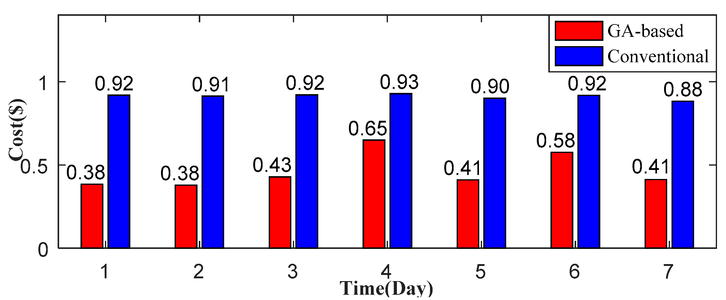
The weekly EWH cost for an entire simulation week given fluctuating electricity price as in Figure 7 is also shown in Figure 14. The cost on EWH for each day is shown in Figure 15. The cost of GA-based power solution is always lower than conventional one for a week-long simulation. On a demo week given the usage pattern from [31], a residential home using 558 gallons of hot water will pay $3.24. The user can save 49.2% of the cost on EWH.
6. Conclusions
Under a day-ahead, dynamic electricity price framework, there is huge potential to save the energy cost of residential appliances. The main goal of this paper is to find an optimal power solution to minimize the cost spent on residential EWH.
First, this paper proposed and tested an adaptive NARX model of EWH. The aim of developing learning-based model is to obtain an accurate model that can be adaptive to seasonal change, climate change and resident changes.
This paper also analyzed several forecasting method on residential hot water consumption pattern and developed a seasonal ARIMA model for DSM. The accuracy of the forecasting is closely related to the optimization of energy solution and the satisfaction of the user’s experience.
Finally, a GA-based algorithm is developed to find the optimal power solution for managing EWH energy consumption with minimum cost. The results show that users can have a huge benefit by changing from conventional method to the proposed algorithm. The paper also considered and analyzed the PAPR from the stand point of the utility company.
Future work may include continuous optimization of consecutive hours instead of 24-h frame, detailed compensating methods for prediction error and new applications of the proposed mechanism for other appliances and for smart neighborhood system as one intergraded system.
Author Contributions
Bo Lin and Shuhui Li conceived and designed the experiments; Bo Lin performed the experiments; Bo Lin, Shuhui Li and Yang Xiao analyzed the data; Bo Lin and Shuhui Li wrote the paper.
Conflicts of Interest
The authors declare no conflict of interest.
References
- Qdr, Q. Benefits of Demand Response in Electricity Markets and Recommendations for Achieving Them; Technical Report; US Department of Energy: Washington, DC, USA, 2006.
- Outlook, A.E. Early Release: Annotated Summary of Two Cases; DOE/EIA-440 0373ER; US Energy Information Administration: Washington, DC, USA, 2016.
- Zhang, D.; Li, S.; Sun, M.; O’Neill, Z. An optimal and learning-based demand response and home energy management system. IEEE Trans. Smart Grid 2016, 7, 1790–1801. [Google Scholar] [CrossRef]
- Goddard, G.; Klose, J.; Backhaus, S. Model development and identification for fast demand response in commercial hvac systems. IEEE Trans. Smart Grid 2014, 5, 2084–2092. [Google Scholar] [CrossRef]
- Kepplinger, P.; Huber, G.; Petrasch, J. Autonomous optimal control for demand side management with resistive domestic hot water heaters using linear optimization. Energy Build. 2015, 100, 50–55. [Google Scholar] [CrossRef]
- Wang, Y.; Lin, X.; Pedram, M. A near-optimal model-based control algorithm for households equipped with residential photovoltaic power generation and energy storage systems. IEEE Trans. Sustain. Energy 2016, 7, 77–86. [Google Scholar] [CrossRef]
- Du, P.; Lu, N. Appliance commitment for household load scheduling. IEEE Trans. Smart Grid 2011, 2, 411–419. [Google Scholar] [CrossRef]
- Gelažanskas, L.; Gamage, K.A. Distributed energy storage using residential hot water heaters. Energies 2016, 9, 127. [Google Scholar]
- Xu, Z.; Diao, R.; Lu, S.; Lian, J.; Zhang, Y. Modeling of electric water heaters for demand response: A baseline pde model. IEEE Trans. Smart Grid 2014, 5, 2203–2210. [Google Scholar] [CrossRef]
- Belov, A.; Kartak, V.; Vasenev, A.; Meratnia, N.; Havinga, P.J. Load shifting of domestic water heaters under double price tariffs: Bringing together money savings and comfort. In Proceedings of the IEEE PES Innovative Smart Grid Technologies Conference Europe (ISGT-Europe), Ljubljana, Slovenia, 9–12 October 2016; pp. 1–6. [Google Scholar]
- Belov, A.; Vasenev, A.; Kartak, V.; Meratnia, N.; Havinga, P.J. Peak load reduction of multiple water heaters: Respecting consumer comfort and money savings. In Proceedings of the 2016 IEEE Online Conference on Green Communications (OnlineGreenComm), Piscataway, NJ, USA, 14 November–17 December 2016; pp. 51–57. [Google Scholar]
- Sen, M. Mathematical Analysis of Engineering Systems; Department of Aerospace and Mechanical Engineering, University of Notre Dame: Notre Dame, IN, USA, 2008. [Google Scholar]
- Barteczko-Hibbert, C.; Gillott, M.; Kendall, G. An artificial neural network for predicting domestic hot water characteristics. Int. J. Low-Carbon Technol. 2009, 4, 112–119. [Google Scholar] [CrossRef]
- A.O. Smith Corp. Introduction Residential Sizing Design Factors—A.O. Smith Water Heaters. Available online: http://www.hotwater.com/lit/sizing/aossg88150.pdf (accessed on 1 August 2017).
- Pollard, A.; Stoecklein, A.; Camilleri, M.; Amitrano, L.; Isaacs, N. An initial investigation into new zealand’s residential hot water energy usage. In Proceedings of the 2001 IRHACE Conference, Palmerston North, New Zealand, March 2001. [Google Scholar]
- Meng, F.-L.; Zeng, X.-J. A profit maximization approach to demand response management with customers behavior learning in smart grid. IEEE Trans. Smart Grid 2016, 7, 1516–1529. [Google Scholar] [CrossRef]
- Gelazanskas, L.; Gamage, K.A.A. Forecasting hot water consumption in residential houses. Energies 2015, 8, 12702–12717. [Google Scholar] [CrossRef] [Green Version]
- Hermansson, T. Analysis of Load Curves in One-Family Houses Using Artificial Neural Networks, School of Mechanical Engineering; Energy Economics and Planning, Department of Heat & Power Engineering, Lund Institute of Technology/Lund University: Lund, Sweden, 2004. [Google Scholar]
- Holcomb, F.H.; Massie, D.D.; Kang, J.H.; Boettner, D.D.; Knight, J.L. Validation of Combined Heat and Power (chp) Models to Field Data for a Residential Proton Exchange Fuel Cell (pem) Demonstration; Engineer Research and Development Center Champaign IL Construction Engineering Research Lab: Champaign, IL, USA, 2004. [Google Scholar]
- Lomet, A.; Suard, F.; Chèze, D. Statistical modeling for real domestic hot water consumption forecasting. Energy Procedia 2015, 70, 379–387. [Google Scholar] [CrossRef]
- Chen, G.; Abraham, B.; Bennett, G.W. Parametric and non-parametric modelling of time series—An empirical study. Environmetrics 1997, 8, 63–74. [Google Scholar] [CrossRef]
- Hong, T.; Wilson, J.; Xie, J. Long term probabilistic load forecasting and normalization with hourly information. IEEE Trans. Smart Grid 2014, 5, 456–462. [Google Scholar] [CrossRef]
- Energy, A.F. Real-Time Pricing for Residential Customers. Available online: https://www2.ameren.com/RetailEnergy/RealTimePrices (accessed on 1 August 2017).
- Li, S.; Zhang, D. Developing smart and real-time demand response mechanism for residential energy consumers. In Proceedings of the Power Systems Conference (PSC), 2014 Clemson University, Clemson, SC, USA, 11–14 March 2014; pp. 1–5. [Google Scholar]
- Sudhoff, S.; Lee, Y. Genetic Optimization System Engineering Toolbox 2.6 (Goset:Version 2.6); Purdue University: West Lafayette, IN, USA, 2016. [Google Scholar]
- Rosin, A.; Hõimoja, H.; Möller, T.; Lehtla, M. Residential electricity consumption and loads pattern analysis. In Proceedings of the Electric Power Quality and Supply Reliability Conference (PQ), Kuressaare, Estonia, 16–18 June 2010; pp. 111–116. [Google Scholar]
- Liu, Y.; Yuen, C.; Huang, S.; Hassan, N.U.; Wang, X.; Xie, S. Peak-to-average ratio constrained demand-side management with consumer’s preference in residential smart grid. IEEE J. Sel. Top. Signal Process. 2014, 8, 1084–1097. [Google Scholar] [CrossRef]
- Nguyen, H.K.; Song, J.B.; Han, Z. Demand side management to reduce peak-to-average ratio using game theory in smart grid. In Proceedings of the 2012 IEEE Conference on Computer Communications Workshops (INFOCOM WKSHPS), Orlando, FL, USA, 25–30 March 2012; pp. 91–96. [Google Scholar]
- eia. Prices and Factors Affecting Prices. Available online: https://www.eia.gov/energyexplained/index.cfm?page=electricity_factors_affecting_prices (accessed on 1 August 2017).
- Hossain, E.; Han, Z.; Poor, H.V. Smart Grid Communications and Networking; Cambridge University Press: Cambridge, UK, 2012. [Google Scholar]
- George, D.; Pearre, N.S.; Swan, L.G. High resolution measured domestic hot water consumption of canadian homes. Energy Build. 2015, 109, 304–315. [Google Scholar] [CrossRef]
- Nehrir, M.H.; Jia, R.; Pierre, D.A.; Hammerstrom, D.J. Power management of aggregate electric water heater loads by voltage control. In Proceedings of the Power Engineering Society General Meeting, Tampa, FL, USA, 24–28 June 2007; pp. 1–6. [Google Scholar]
- Richardson, I.; Thomson, M. Domestic Electricity Demand Model—Simulation Example; Loughborough University: Loughborough, UK, 2010. [Google Scholar]
- Samadi, P.; Mohsenian-Rad, H.; Schober, R.; Wong, V.W. Advanced demand side management for the future smart grid using mechanism design. IEEE Trans. Smart Grid 2012, 3, 1170–1180. [Google Scholar] [CrossRef]
Figure 1.
(a) Structure of electric water heater; and (b) traditional on/off control method illustration.
Figure 1.
(a) Structure of electric water heater; and (b) traditional on/off control method illustration.
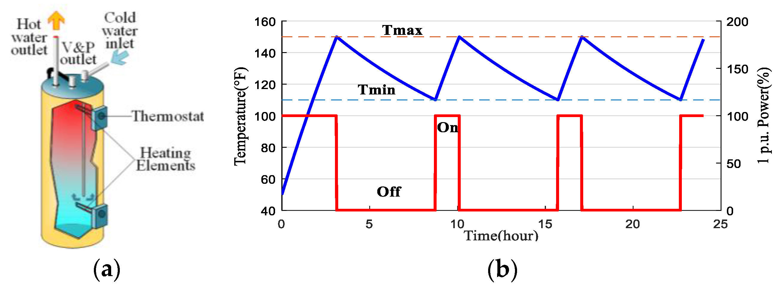
Figure 2.
EWH simulation system in Simulink MATLAB.

Figure 3.
NARX network structure.

Figure 4.
NARX training performance for: (a) training dataset; (b) validation dataset; (c) test dataset; and (d) overall dataset.
Figure 4.
NARX training performance for: (a) training dataset; (b) validation dataset; (c) test dataset; and (d) overall dataset.

Figure 5.
Maximum capability given different tank temperature and input power with base temperature set at 110 °F.
Figure 5.
Maximum capability given different tank temperature and input power with base temperature set at 110 °F.

Figure 6.
Forecast of water demand with different methods targeting data from GEFCom2014.
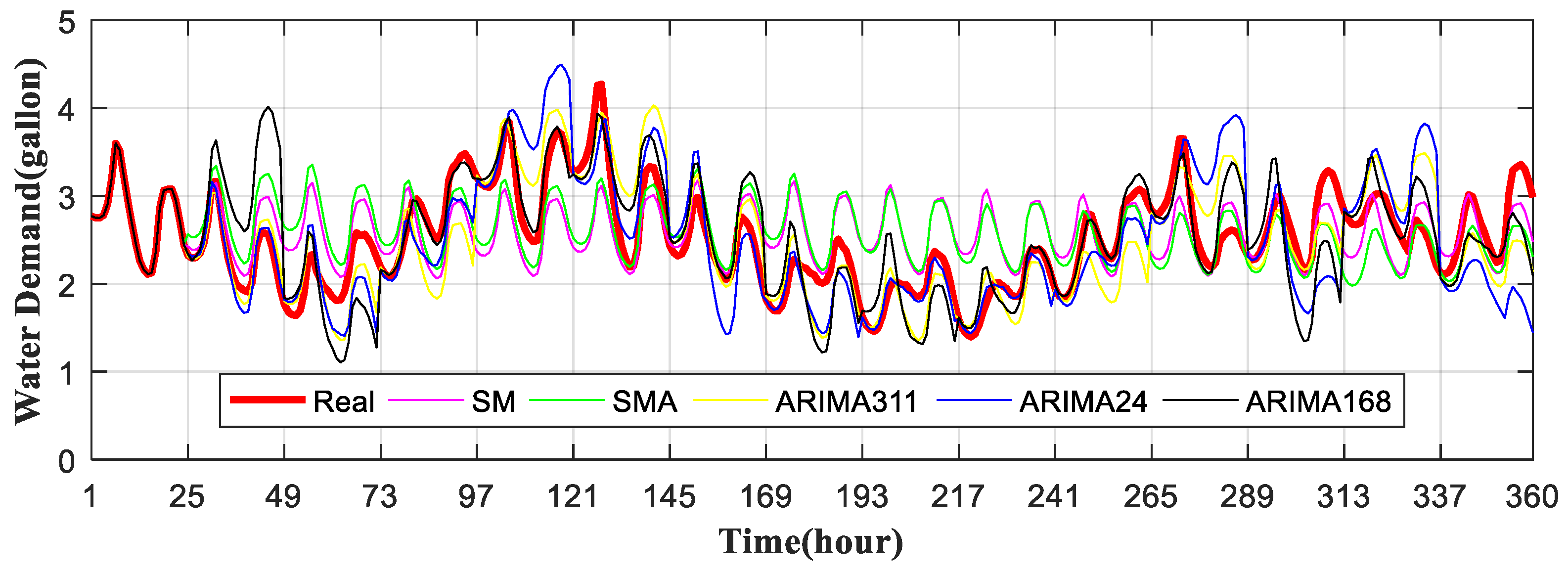
Figure 7.
Forecast of water demand with different methods targeting data from GEFCom2014.

Figure 8.
The 24-h water demand pattern.

Figure 9.
Comparison of EWH power consumption solution.

Figure 10.
Comparison of EWH water demand and maximum capability.

Figure 11.
The 24-h EWH tank temperature.

Figure 12.
Load simulation of a residential house.

Figure 13.
Comparison of load difference between GA-based and conventional.
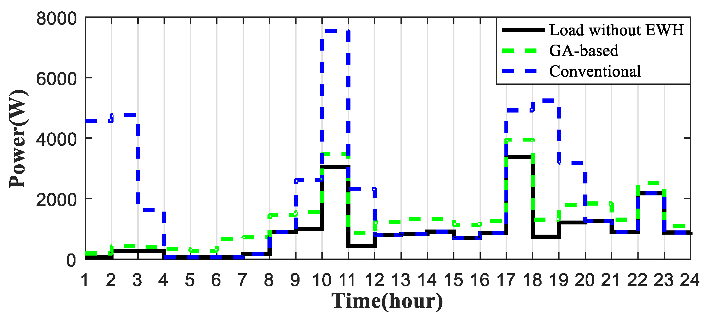
Figure 14.
Comparison of weekly cost and PAPR between GA-based and conventional.
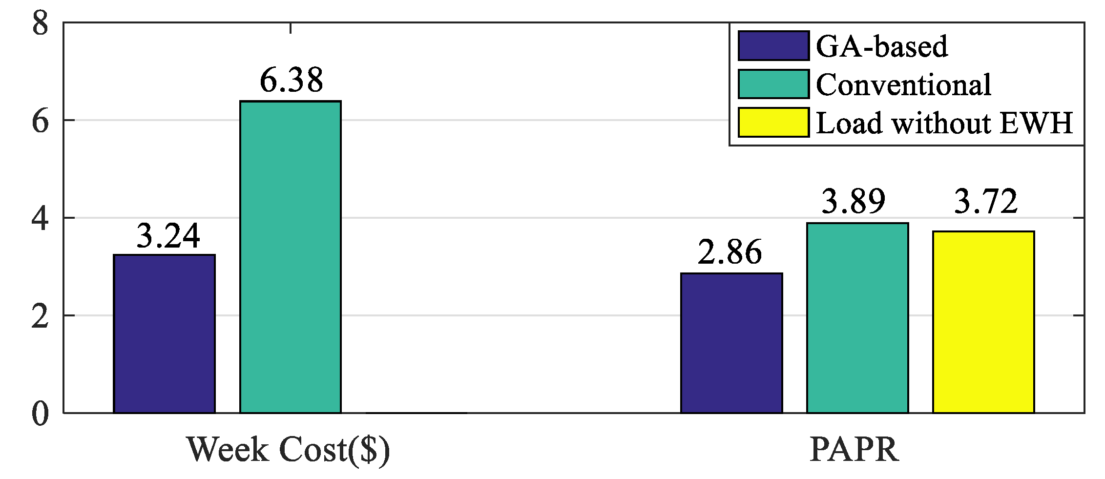
Figure 15.
Comparison of daily cost between GA-based and conventional.


Table 1.
Neural Network modeling input and target data (Note: T(°C) = (T(°F) − 32) × 5/9, 1 gallon = 0.00378541 m3).
Table 1.
Neural Network modeling input and target data (Note: T(°C) = (T(°F) − 32) × 5/9, 1 gallon = 0.00378541 m3).
| Input | Target | ||||
|---|---|---|---|---|---|
| Tank Temperature (°F) | Power Input (W) | Water Demand (gal) | Inlet Water Temperature (°F) | Ambient Temperature (°F) | Outlet Water Temperature (°F) |
| 162.43 | 3643.5 | 1.17 | 48.80 | 51.64 | 179.81 |
| 179.81 | 789.5 | 3.18 | 48.50 | 51.61 | 171.01 |
| 171.01 | 276.4 | 1.78 | 48.53 | 48.33 | 160.50 |
| 160.50 | 1893.7 | 3.34 | 49.50 | 46.46 | 161.80 |
| 161.80 | 278.2 | 4.24 | 49.80 | 53.94 | 149.91 |
| 149.91 | 1655.4 | 2.70 | 50.65 | 51.85 | 151.20 |
Table 2.
Model Fitting Results for EWH Consumption.
| Method | Performance Measures | ||
|---|---|---|---|
| nMAE | nRMSE | MASE | |
| Seasonal Mean | 0.7502 | 0.9182 | 0.9743 |
| MA 24 | 0.8213 | 0.9683 | 0.9638 |
| ARIMA (3,1,1) with SMA 24 | 0.6045 | 0.7708 | 0.7851 |
| ARIMA (1,1,1) (1,0,2)24 | 0.6756 | 0.9571 | 0.8774 |
| ARIMA (1,1,2) (1,0,0)168 | 0.5815 | 0.8112 | 0.6824 |
© 2017 by the authors. Licensee MDPI, Basel, Switzerland. This article is an open access article distributed under the terms and conditions of the Creative Commons Attribution (CC BY) license (http://creativecommons.org/licenses/by/4.0/).
Share and Cite
MDPI and ACS Style
Lin, B.; Li, S.; Xiao, Y. Optimal and Learning-Based Demand Response Mechanism for Electric Water Heater System. Energies 2017, 10, 1722. https://doi.org/10.3390/en10111722
AMA Style
Lin B, Li S, Xiao Y. Optimal and Learning-Based Demand Response Mechanism for Electric Water Heater System. Energies. 2017; 10(11):1722. https://doi.org/10.3390/en10111722
Chicago/Turabian StyleLin, Bo, Shuhui Li, and Yang Xiao. 2017. "Optimal and Learning-Based Demand Response Mechanism for Electric Water Heater System" Energies 10, no. 11: 1722. https://doi.org/10.3390/en10111722
Note that from the first issue of 2016, this journal uses article numbers instead of page numbers. See further details here.