Devising Hourly Forecasting Solutions Regarding Electricity Consumption in the Case of Commercial Center Type Consumers

 ,
,  ,
,  ,
,  ,
,
Abstract
:
1. Introduction
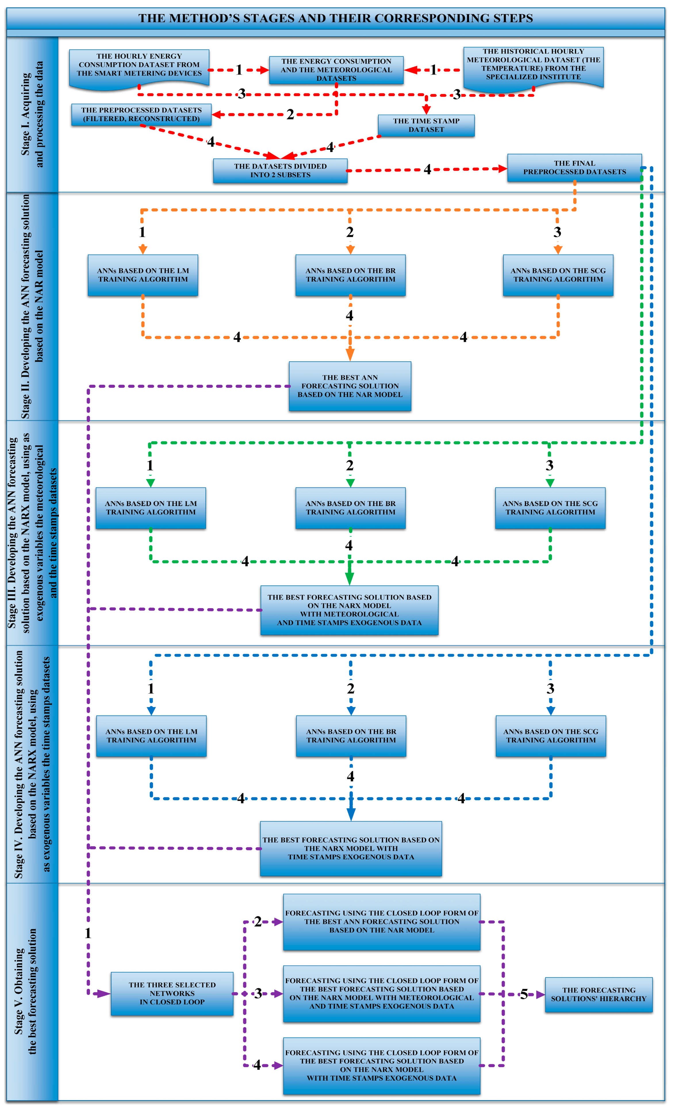
2. Materials and Methods
2.1. Acquiring and Processing the Data
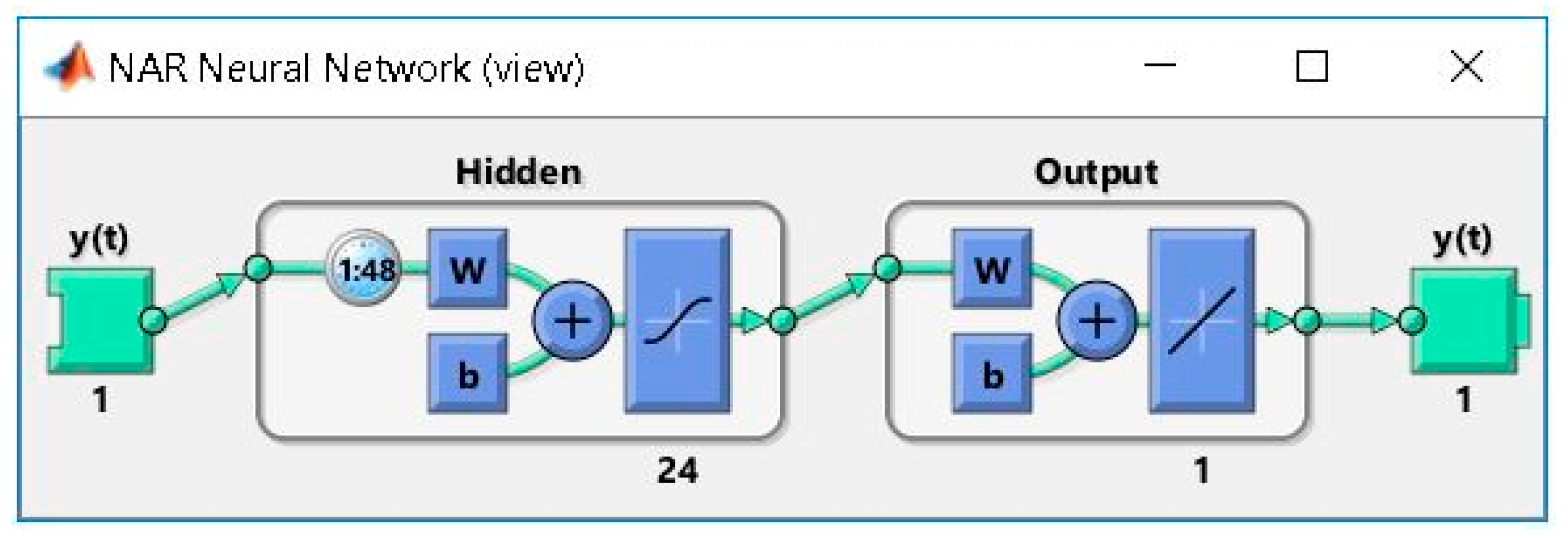
2.2. Developing the ANN Forecasting Solution Based on the NAR Model
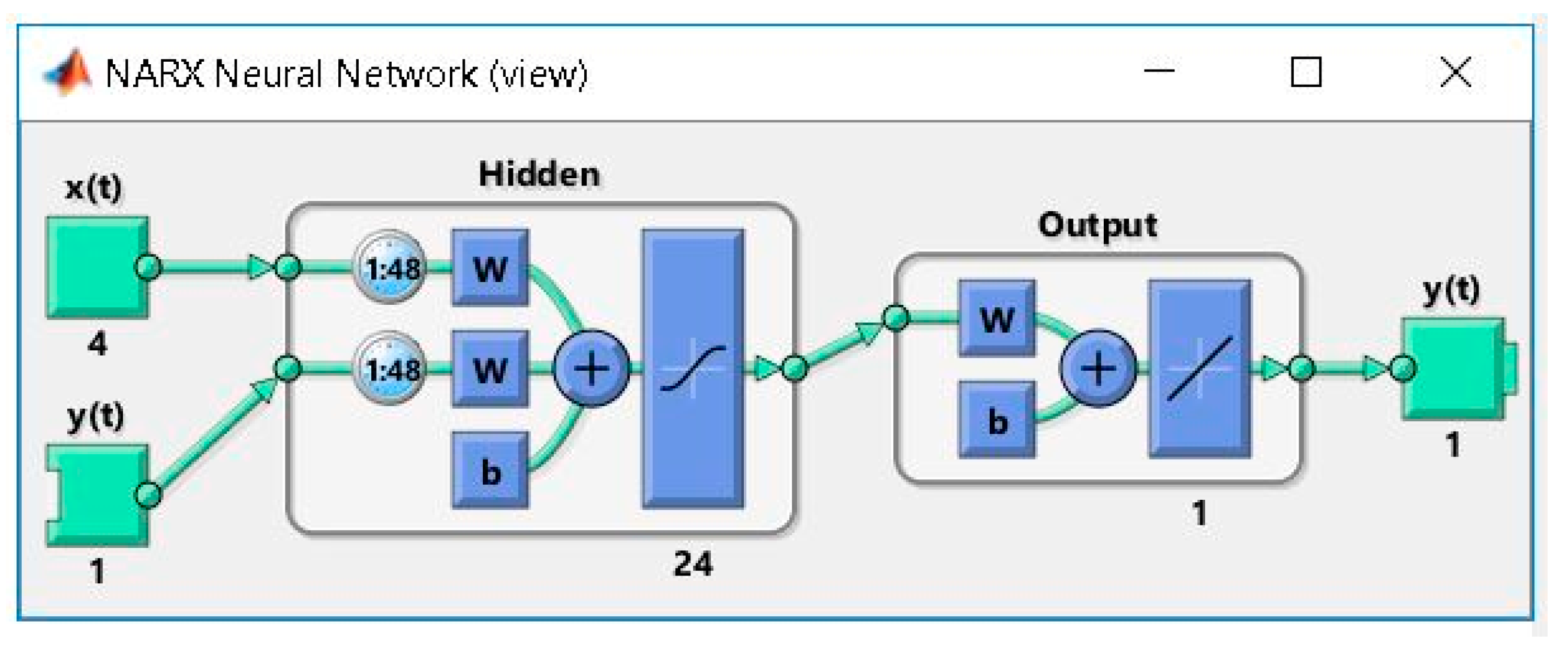
2.3. Developing the ANN Forecasting Solution Based on the NARX Model, Using as Exogenous Variables the Meteorological and the Time Stamps Datasets
2.4. Developing the ANN Forecasting Solution Based on the NARX Model, Using as Exogenous Variables the Time Stamps Datasets
2.5. Obtaining the Best Forecasting Solution
3. Results
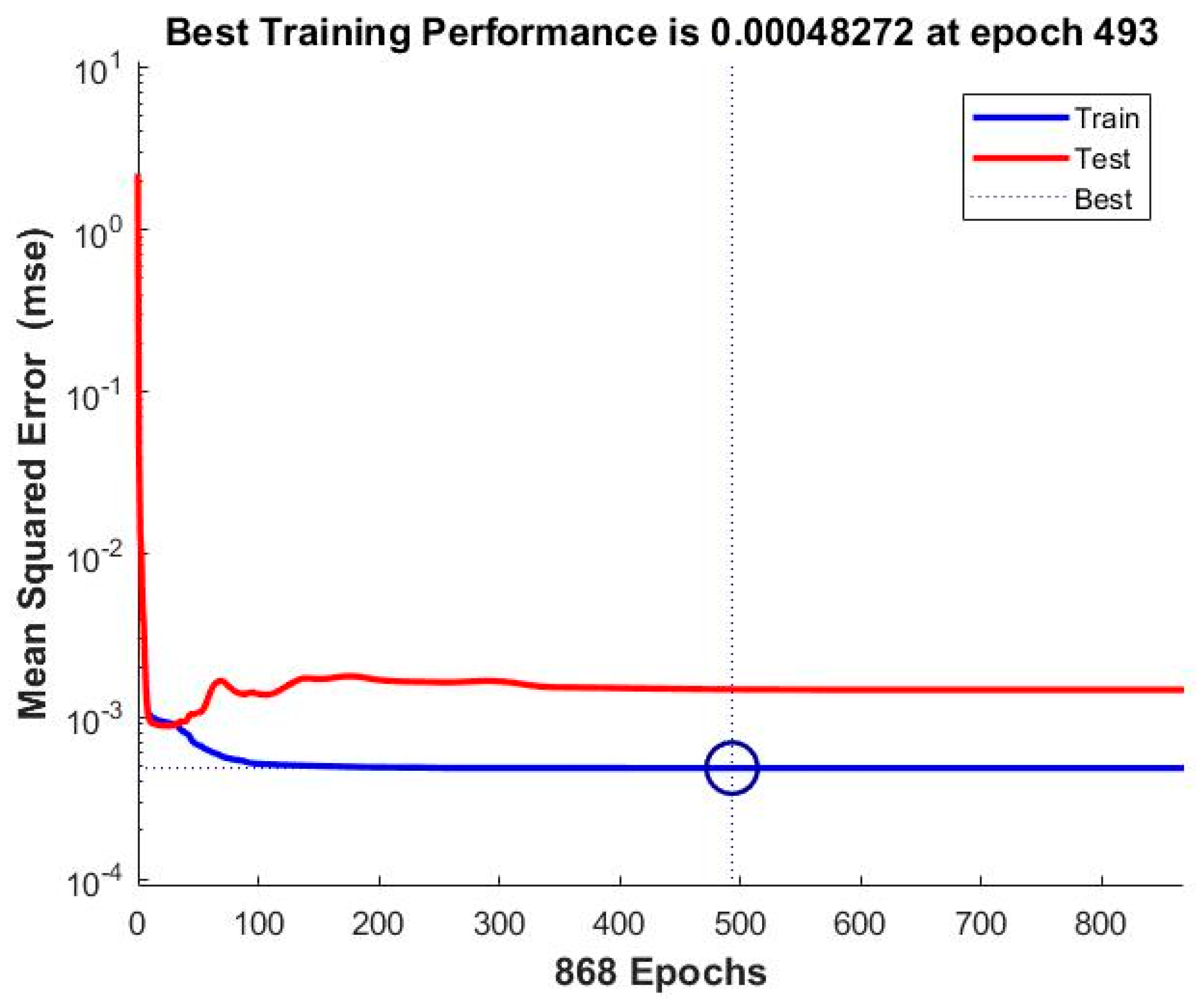
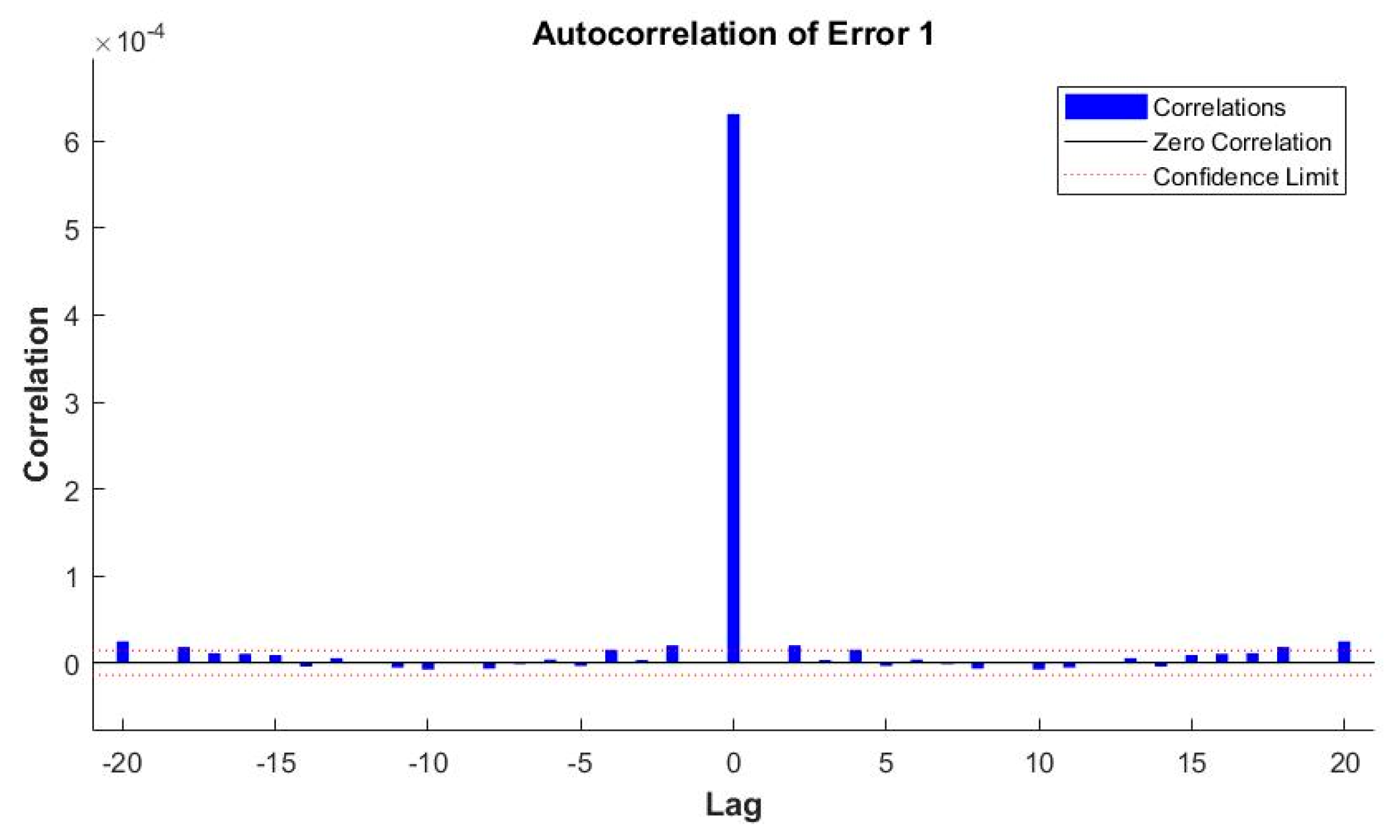
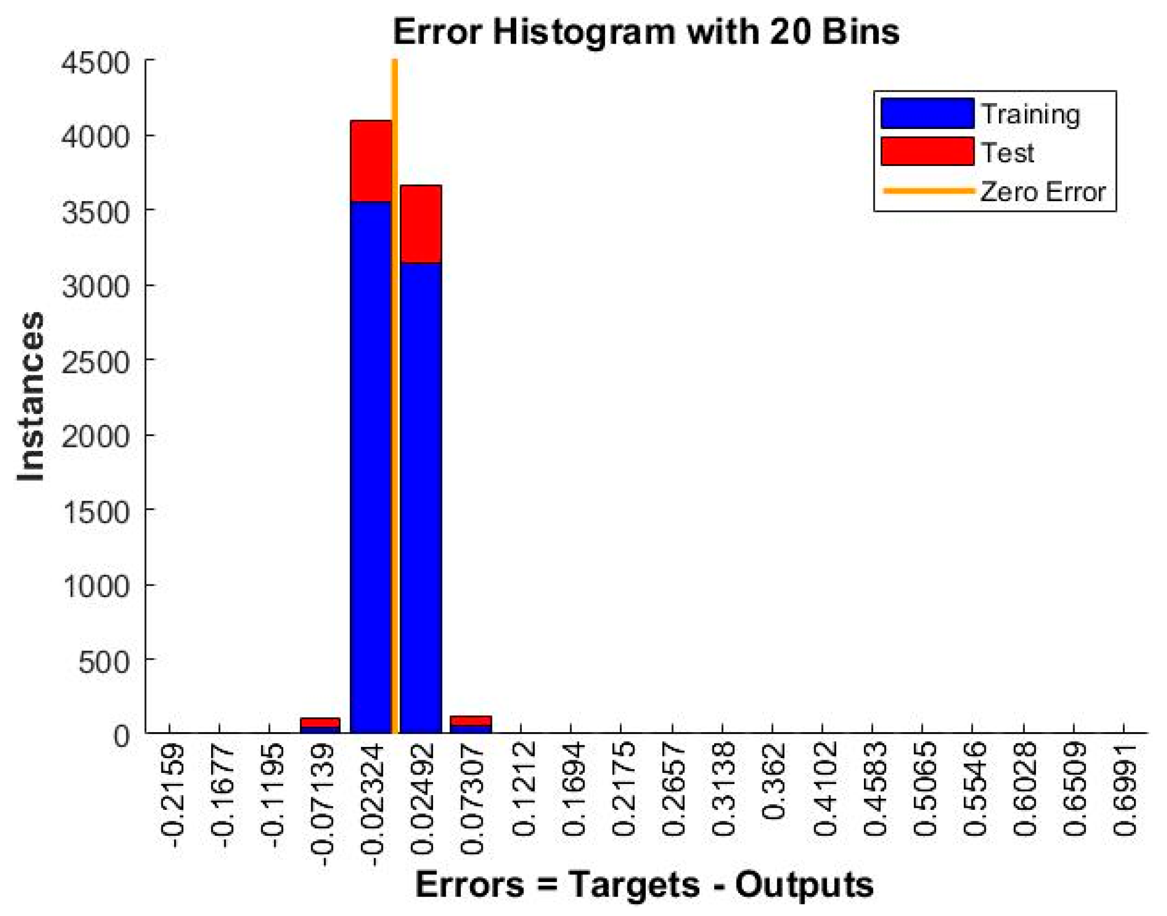
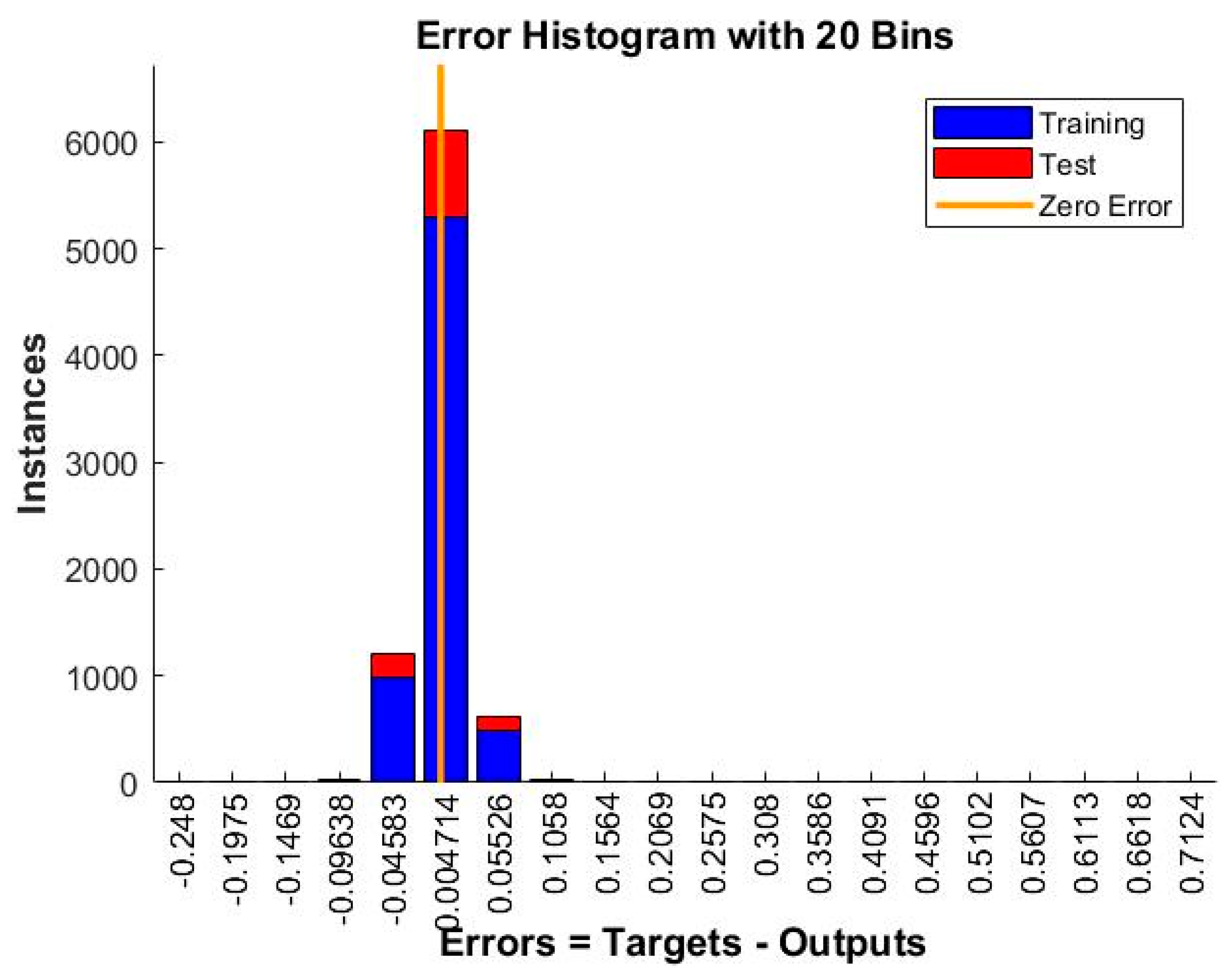
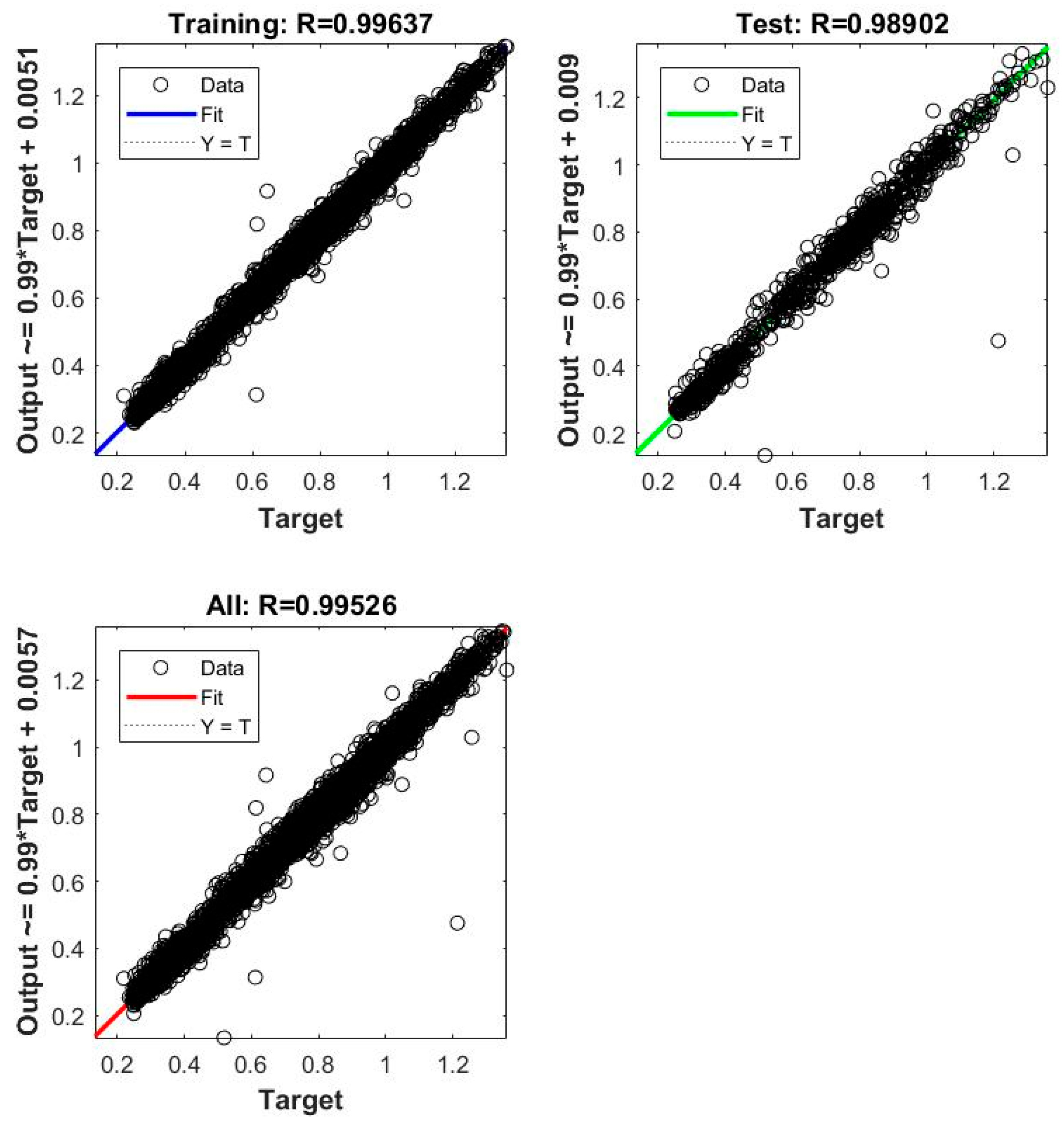
3.1. Results Regarding the Developed ANN Forecasting Solution Based on the NAR Model
3.2. Results Regarding the Developed ANN Forecasting Solution Based on the NARX Model, Using as Exogenous Variables the Meteorological and the Time Stamps Datasets
3.3. Results Regarding the Developed ANN Forecasting Solution Based on the NARX Model, Using as Exogenous Variables the Time Stamps Datasets
3.4. Results Concerning the Best Forecasting Solution
4. Discussion
5. Conclusions
Supplementary Materials
Acknowledgments
Author Contributions
Conflicts of Interest
References
- World Energy Balances: Overview (2017 Edition). Available online: http://www.iea.org/publications/freepublications/publication/WorldEnergyBalances2017Overview.pdf (accessed on 9 January 2017).
- Rigatos, G. Advanced Models of Neural Networks: Nonlinear Dynamics and Stochasticity in Biological Neurons; Springer: Berlin, Germany, 2015; ISBN 9783662437636. [Google Scholar]
- Krawczak, M. Multilayer Neural Networks: A Generalized Net Perspective; Springer Publishing Company: Heidelberg, Germany, 2013; ISBN 978-3-319-00248-4. [Google Scholar]
- Chakraverty, S.; Mall, S. Artificial Neural Networks for Engineers and Scientists: Solving Ordinary Differential Equations; CRC Press: Boca Raton, FL, USA, 2017; ISBN 9781351651318. [Google Scholar]
- Da Silva, I.N.; Spatti, D.H.; Flauzino, R.A.; Liboni, L.H.B.; dos Reis Alves, S.F. Artificial Neural Networks: A Practical Course; Springer International Publishing: Basel, Switzerland, 2016; ISBN 9783319431628. [Google Scholar]
- Goodfellow, I.; Bengio, Y.; Courville, A. Deep Learning (Adaptive Computation and Machine Learning Series); MIT Press: Cambridge, UK, 2016; ISBN 9780262035613. [Google Scholar]
- Almonacid, F.; Fernandez, E.F.; Mellit, A.; Kalogirou, S. Review of techniques based on artificial neural networks for the electrical characterization of concentrator photovoltaic technology. Renew. Sustain. Energy Rev. 2017, 75, 938–953. [Google Scholar] [CrossRef]
- Qazi, A.; Fayaz, H.; Wadi, A.; Raj, R.G.; Rahim, N.A.; Khan, W.A. The artificial neural network for solar radiation prediction and designing solar systems: A systematic literature review. J. Clean. Prod. 2015, 104, 1–12. [Google Scholar] [CrossRef]
- Yadav, A.K.; Chandel, S.S. Solar radiation prediction using Artificial Neural Network techniques: A review. Renew. Sustain. Energy Rev. 2014, 33, 772–781. [Google Scholar] [CrossRef]
- Du, K.L.; Swamy, M.N.S. Neural Networks and Statistical Learning; SpringerLink: London, UK, 2013; ISBN 9781447155713. [Google Scholar]
- Kumar, R.; Aggarwal, R.K.; Sharma, J.D. Comparison of regression and artificial neural network models for estimation of global solar radiations. Renew. Sustain. Energy Rev. 2015, 52, 1294–1299. [Google Scholar] [CrossRef]
- Yadav, A.K.; Chandel, S.S. Identification of relevant input variables for prediction of 1-minute time-step photovoltaic module power using Artificial Neural Network and Multiple Linear Regression Models. Renew. Sustain. Energy Rev. 2017, 77, 955–969. [Google Scholar] [CrossRef]
- Paliwal, M.; Kumar, U.A. Neural networks and statistical techniques: A review of applications. Expert Syst. Appl. 2009, 36, 2–17. [Google Scholar] [CrossRef]
- Bou-rabee, M.; Sulaiman, S.A.; Saleh, M.S.; Mara, S. Using artificial neural networks to estimate solar radiation in Kuwait. Renew. Sustain. Energy Rev. 2017, 72, 434–438. [Google Scholar] [CrossRef]
- Xiao, Q.; Xing, L.; Song, G. Time series prediction using optimal theorem and dynamic Bayesian network. Opt. Int. J. Light Electron Opt. 2016, 127, 11063–11069. [Google Scholar] [CrossRef]
- Proskuryakov, A. Intelligent System for Time Series Forecasting. Procedia Comput. Sci. 2017, 103, 363–369. [Google Scholar] [CrossRef]
- Xiao, Q. Time series prediction using bayesian filtering model and fuzzy neural networks. Opt. Int. J. Light Electron Opt. 2017, 140, 104–113. [Google Scholar] [CrossRef]
- Tealab, A.; Hefny, H.; Badr, A. Forecasting of nonlinear time series using ANN. Future Comput. Inform. J. 2017, 2, 39–47. [Google Scholar] [CrossRef]
- Ibrahim, M.; Jemei, S.; Wimmer, G.; Hissel, D. Nonlinear autoregressive neural network in an energy management strategy for battery/ultra-capacitor hybrid electrical vehicles. Electr. Power Syst. Res. 2016, 136, 262–269. [Google Scholar] [CrossRef]
- Yang, D.; Dong, Z.; Lim, L.H.I.; Liu, L. Analyzing big time series data in solar engineering using features and PCA. Sol. Energy 2017, 153, 317–328. [Google Scholar] [CrossRef]
- Hirata, Y.; Aihara, K. Improving time series prediction of solar irradiance after sunrise: Comparison among three methods for time series prediction. Sol. Energy 2017, 149, 294–301. [Google Scholar] [CrossRef]
- Zheng, T.; Chen, R. Dirichlet ARMA models for compositional time series. J. Multivar. Anal. 2017, 158, 31–46. [Google Scholar] [CrossRef]
- Deb, C.; Zhang, F.; Yang, J.; Lee, S.E.; Shah, K.W. A review on time series forecasting techniques for building energy consumption. Renew. Sustain. Energy Rev. 2017. [Google Scholar] [CrossRef]
- Balestrassi, P.P.; Popova, E.; Paiva, A.P.; Marangon Lima, J.W. Design of experiments on neural network’s training for nonlinear time series forecasting. Neurocomputing 2009, 72, 1160–1178. [Google Scholar] [CrossRef]
- Benmouiza, K.; Cheknane, A. Forecasting hourly global solar radiation using hybrid k-means and nonlinear autoregressive neural network models. Energy Convers. Manag. 2013, 75, 561–569. [Google Scholar] [CrossRef]
- Wong, S.L.; Wan, K.K.W.; Lam, T.N.T. Artificial neural networks for energy analysis of office buildings with daylighting. Appl. Energy 2010, 87, 551–557. [Google Scholar] [CrossRef]
- Mocanu, E.; Nguyen, P.H.; Gibescu, M.; Kling, W.L. Comparison of machine learning methods for estimating energy consumption in buildings. In Proceedings of the 13th International Conference on Probabilistic Methods Applied to Power Systems, Durham, UK, 7–10 July 2014. [Google Scholar]
- Esener, I.I.; Yüksel, T.; Kurban, M. Short-term load forecasting without meteorological data using AI-based structures. Turk. J. Electr. Eng. Comput. Sci. 2015, 23, 370–380. [Google Scholar] [CrossRef]
- Tsekouras, G.J.; Kanellos, F.D.; Mastorakis, N. Short Term Load Forecasting in Electric Power Systems with Artificial Neural Networks. In Computational Problems in Science and Engineering; Mastorakis, N., Bulucea, A., Tsekouras, G., Eds.; Springer International Publishing: Cham, Germany, 2015; pp. 19–58. ISBN 978-3-319-15765-8. [Google Scholar]
- Tanıdır, Ö.; Tor, O.B. Accuracy of ANN based day-ahead load forecasting in Turkish power system: Degrading and improving factors. Neural Netw. World 2015, 25, 443–456. [Google Scholar] [CrossRef]
- Ruiz, L.; Cuéllar, M.; Calvo-Flores, M.; Pegalajar Jiménez, M.; Del, C. An Application of Non-Linear Autoregressive Neural Networks to Predict Energy Consumption in Public Buildings. Energies 2016, 9, 684. [Google Scholar] [CrossRef]
- Sun, C.; Sun, F.; Moura, S.J. Nonlinear predictive energy management of residential buildings with photovoltaics & batteries. J. Power Sources 2016, 325, 723–731. [Google Scholar] [CrossRef]
- Bogomolov, A.; Lepri, B.; Larcher, R.; Antonelli, F.; Pianesi, F.; Pentland, A. Energy consumption prediction using people dynamics derived from cellular network data. EPJ Data Sci. 2016, 5. [Google Scholar] [CrossRef]
- Mauledoux, M.; Aviles, O.; Mejia-Ruda, E.; Caldas, O.I. Analysis of autoregressive predictive models and artificial neural networks for irradiance estimation. Indian J. Sci. Technol. 2016, 9. [Google Scholar] [CrossRef]
- Buitrago, J.; Asfour, S. Short-term forecasting of electric loads using nonlinear autoregressive artificial neural networks with exogenous vector inputs. Energies 2017, 10. [Google Scholar] [CrossRef]
- Gajowniczek, K.; Zabkowski, T. Electricity forecasting on the individual household level enhanced based on activity patterns. PLoS ONE 2017, 12. [Google Scholar] [CrossRef] [PubMed]
- Levenberg, K. A method for the solution of certain non-linear problems in least squares. Q. J. Appl. Math. 1944, 2, 164–168. [Google Scholar] [CrossRef]
- Marquardt, D.W. An Algorithm for Least-Squares Estimation of Nonlinear Parameters. J. Soc. Ind. Appl. Math. 1963, 11, 431–441. [Google Scholar] [CrossRef]
- Kişi, Ö.; Uncuoǧlu, E. Comparison of three back-propagation training algorithms for two case studies. Indian J. Eng. Mater. Sci. 2005, 12, 434–442. [Google Scholar]
- Neural Network Object Properties—MATLAB & Simulink. Available online: https://www.mathworks.com/help/nnet/ug/neural-network-object-properties.html#bss4hk6-48 (accessed on 12 October 2017).
- MacKay, D.J.C. Bayesian Interpolation. Neural Comput. 1992, 4, 415–447. [Google Scholar] [CrossRef]
- Foresee, F.D.; Hagan, M.T. Guass-Newton approximation to bayesian learning. In Proceedings of the International Conference on Neural Networks, Houston, TX, USA, 9–12 June 1997; pp. 1930–1935. [Google Scholar]
- Møller, M.F. A scaled conjugate gradient algorithm for fast supervised learning. Neural Netw. 1993, 6, 525–533. [Google Scholar] [CrossRef]
- Lin, T.; Horne, B.G.; Tino, P.; Giles, C.L. Learning long-term dependencies in NARX recurrent neural networks. IEEE Trans. Neural Netw. 1996, 7, 1329–1338. [Google Scholar] [CrossRef] [PubMed]


| Stage | Step | Final Results of the Stage |
|---|---|---|
| I. Acquiring and processing the data | 1. Acquiring the energy consumption and the meteorological datasets | The final preprocessed datasets |
| 2. Preprocessing the data (filtering, reconstructing) | ||
| 3. Constructing the time stamp dataset | ||
| 4. Dividing datasets into 2 subsets | ||
| II. Developing the ANN forecasting solution based on the NAR model | 1. Developing ANNs based on the LM algorithm | The best forecasting solution |
| 2. Developing ANNs based on the BR algorithm | ||
| 3. Developing ANNs based on the SCG algorithm | ||
| 4. Comparing the forecasting accuracy of the obtained ANNs | ||
| III. Developing the ANN forecasting solution based on the NARX model, using as exogenous variables the meteorological and the time stamps datasets | 1. Developing ANNs based on the LM algorithm | The best forecasting solution |
| 2. Developing ANNs based on the BR algorithm | ||
| 3. Developing ANNs based on the SCG algorithm | ||
| 4. Comparing the forecasting accuracy of the obtained ANNs | ||
| IV. Developing the ANN forecasting solution based on the NARX model, using as exogenous variables the time stamps datasets | 1. Developing ANNs based on the LM algorithm | The best forecasting solution |
| 2. Developing ANNs based on the BR algorithm | ||
| 3. Developing ANNs based on the SCG algorithm | ||
| 4. Comparing the forecasting accuracy of the obtained ANNs | ||
| V. Obtaining the best forecasting solution | 1. The 3 selected networks are put into the closed loop form | The forecasting solutions’ hierarchy |
| 2. Forecasting using the best ANN forecasting solution based on the NAR model that has been put in the closed loop form | ||
| 3. Forecasting using the he best forecasting solution based on the NARX model with meteorological and time stamps exogenous data that has been put in the closed loop form | ||
| 4. Forecasting using the he best forecasting solution based on the NARX model with time stamps exogenous data that has been put in the closed loop form | ||
| 5. Comparing the forecasting results from steps 1–4 |
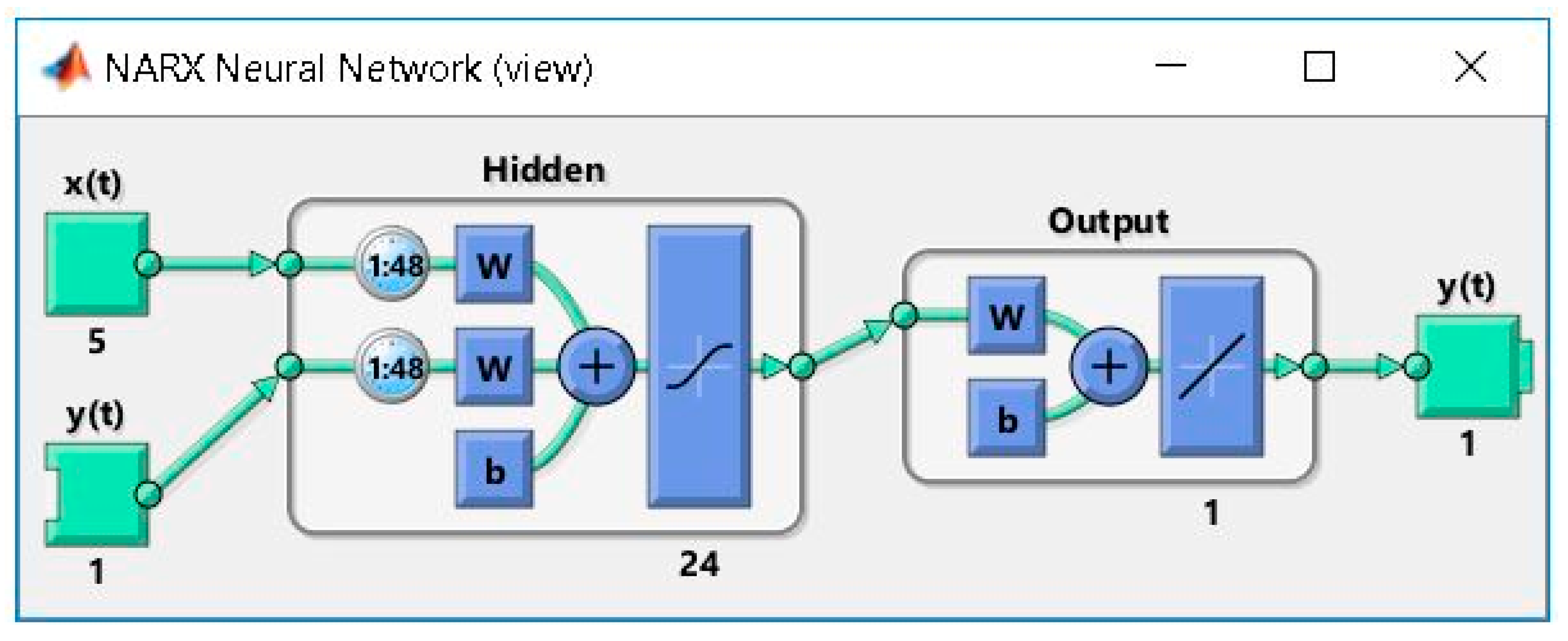
| The Levenberg-Marquardt Training Algorithm | ||||||
| n | d | 2 | 6 | 12 | 24 | 48 |
| 6 | MSE | 0.0029307 | 0.0030022 | 0.0019403 | 0.0018349 | 0.00091808 |
| R | 0.97626 | 0.98049 | 0.9867 | 0.99199 | 0.99272 | |
| 12 | MSE | 0.0025306 | 0.0022852 | 0.0018363 | 0.001085 | 0.0015098 |
| R | 0.97696 | 0.98416 | 0.98811 | 0.99324 | 0.99184 | |
| 24 | MSE | 0.0037219 | 0.0026784 | 0.0013428 | 0.0019062 | 0.0017245 |
| R | 0.97486 | 0.98197 | 0.98986 | 0.99255 | 0.99254 | |
| The Bayesian Regularization Training Algorithm | ||||||
| n | d | 2 | 6 | 12 | 24 | 48 |
| 6 | MSE | 0.0029627 | 0.002228 | 0.0014656 | 0.00094866 | 0.00072544 |
| R | 0.97709 | 0.983 | 0.98909 | 0.99244 | 0.99422 | |
| 12 | MSE | 0.0028051 | 0.0019579 | 0.001046 | 0.00068836 | 0.00056501 |
| R | 0.97871 | 0.98468 | 0.992 | 0.99402 | 0.99448 | |
| 24 | MSE | 0.0026605 | 0.0017508 | 0.00085038 | 0.00057053 | 0.00048272 |
| R | 0.9799 | 0.98549 | 0.99399 | 0.99355 | 0.99526 | |
| The Scaled Conjugate Gradient Training Algorithm | ||||||
| n | d | 2 | 6 | 12 | 24 | 48 |
| 6 | MSE | 0.0035269 | 0.0032701 | 0.0021393 | 0.0015375 | 0.0010847 |
| R | 0.97191 | 0.97206 | 0.98145 | 0.98853 | 0.99123 | |
| 12 | MSE | 0.0052954 | 0.0046987 | 0.0028487 | 0.00093968 | 0.00083771 |
| R | 0.97055 | 0.9691 | 0.98061 | 0.9916 | 0.99241 | |
| 24 | MSE | 0.0038286 | 0.0027353 | 0.0021494 | 0.0016137 | 0.0013316 |
| R | 0.97033 | 0.9762 | 0.9806 | 0.98971 | 0.98819 | |
| The Levenberg-Marquardt Training Algorithm | ||||||
| n | d | 2 | 6 | 12 | 24 | 48 |
| 6 | MSE | 0.0012052 | 0.001088 | 0.00081051 | 0.00080346 | 0.00077934 |
| R | 0.99036 | 0.99218 | 0.99291 | 0.99346 | 0.99394 | |
| 12 | MSE | 0.00080556 | 0.00086619 | 0.00087007 | 0.00070308 | 0.00084926 |
| R | 0.99227 | 0.99254 | 0.99386 | 0.99402 | 0.99375 | |
| 24 | MSE | 0.00085223 | 0.00087959 | 0.00089669 | 0.00096489 | 0.00090853 |
| R | 0.99364 | 0.9926 | 0.99338 | 0.99425 | 0.99401 | |
| The Bayesian Regularization Training Algorithm | ||||||
| n | d | 2 | 6 | 12 | 24 | 48 |
| 6 | MSE | 0.0013377 | 0.0009888 | 0.00071482 | 0.00054033 | 0.00043039 |
| R | 0.98865 | 0.99258 | 0.99387 | 0.99529 | 0.99561 | |
| 12 | MSE | 0.00085773 | 0.00073291 | 0.00054438 | 0.00044708 | 0.00035744 |
| R | 0.9918 | 0.99445 | 0.99555 | 0.9952 | 0.99616 | |
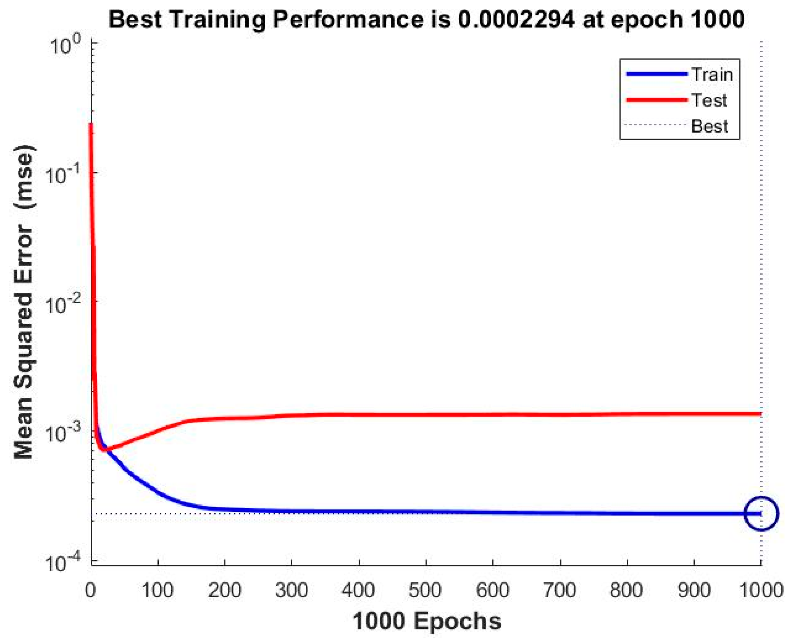
| 24 | MSE | 0.00068362 | 0.00066045 | 0.0004577 | 0.00033796 | 0.0002294 |
| R | 0.99444 | 0.99491 | 0.99578 | 0.9967 | 0.99701 | |
| The Scaled Conjugate Gradient Training Algorithm | ||||||
| n | d | 2 | 6 | 12 | 24 | 48 |
| 6 | MSE | 0.0022016 | 0.0020858 | 0.0012062 | 0.0010987 | 0.00078457 |
| R | 0.98175 | 0.98928 | 0.99079 | 0.99142 | 0.99293 | |
| 12 | MSE | 0.0035236 | 0.002518 | 0.0016623 | 0.00077795 | 0.00088082 |
| R | 0.97808 | 0.98292 | 0.98814 | 0.99254 | 0.99299 | |
| 24 | MSE | 0.0024664 | 0.0014422 | 0.0011421 | 0.00091561 | 0.0011415 |
| R | 0.97996 | 0.98956 | 0.98974 | 0.99227 | 0.99231 | |
| The Levenberg-Marquardt Training Algorithm | ||||||
| n | d | 2 | 6 | 12 | 24 | 48 |
| 6 | MSE | 0.001455 | 0.0019983 | 0.00084518 | 0.00087728 | 0.00084281 |
| R | 0.9878 | 0.99162 | 0.99325 | 0.99266 | 0.9932 | |
| 12 | MSE | 0.00094045 | 0.0012128 | 0.00096237 | 0.00076798 | 0.0009589 |
| R | 0.99159 | 0.99163 | 0.99347 | 0.99388 | 0.99382 | |
| 24 | MSE | 0,00098655 | 0.0011564 | 0.0018315 | 0.0018474 | 0.0010069 |
| R | 0.99288 | 0.99228 | 0.99377 | 0.99306 | 0.99352 | |
| The Bayesian Regularization Training Algorithm | ||||||
| n | d | 2 | 6 | 12 | 24 | 48 |
| 6 | MSE | 0.001611 | 0.0010559 | 0.00072309 | 0.00061356 | 0.00050737 |
| R | 0.98814 | 0.99231 | 0.99393 | 0.99459 | 0.99543 | |
| 12 | MSE | 0.00086453 | 0.00075894 | 0.00058258 | 0.00047763 | 0.00038671 |
| R | 0.99256 | 0.99317 | 0.99475 | 0.995 | 0.99597 | |
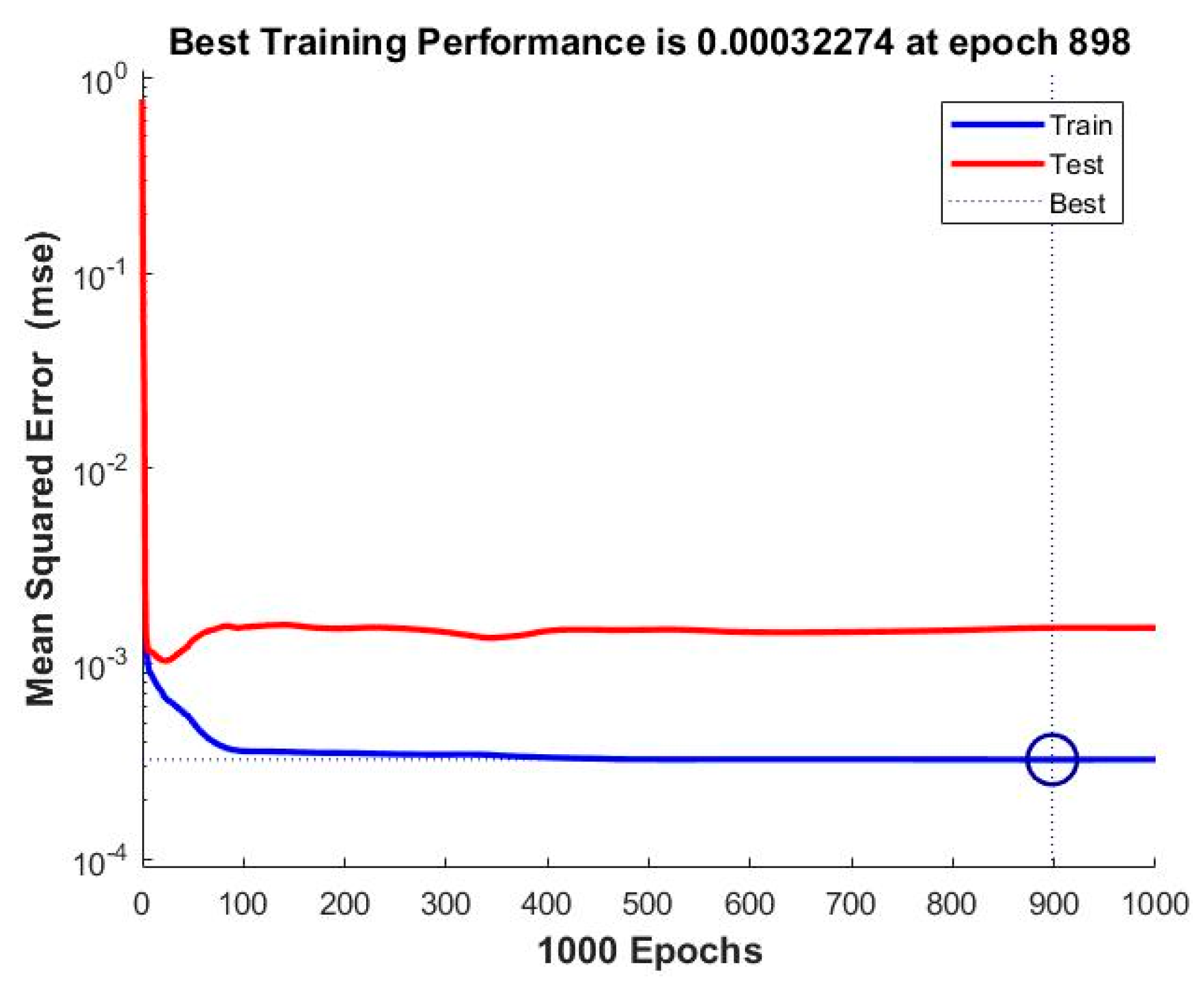
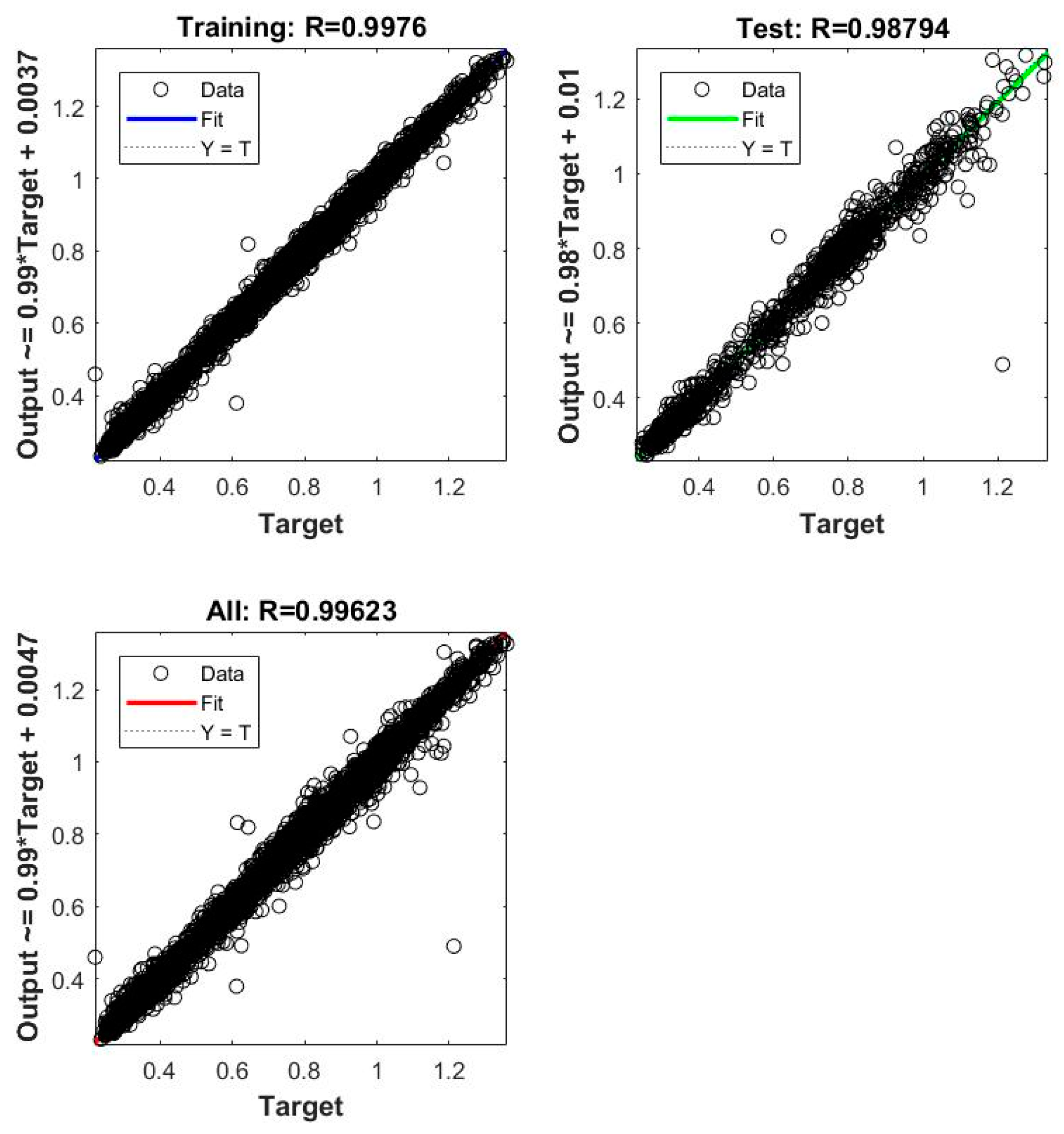
| 24 | MSE | 0.00070019 | 0.00066089 | 0.00049556 | 0.00039866 | 0.00032274 |
| R | 0.99456 | 0.99381 | 0.9948 | 0.99604 | 0.99623 | |
| The Scaled Conjugate Gradient Training Algorithm | ||||||
| n | d | 2 | 6 | 12 | 24 | 48 |
| 6 | MSE | 0.0026367 | 0.0019962 | 0.001349 | 0.001295 | 0.0009588 |
| R | 0.97828 | 0.98305 | 0.98974 | 0.99148 | 0.99208 | |
| 12 | MSE | 0.0039318 | 0.0028443 | 0.002392 | 0.00085282 | 0.000881 |
| R | 0.97681 | 0.98497 | 0.98638 | 0.99254 | 0.99231 | |
| 24 | MSE | 0.0036967 | 0.0016997 | 0.0013259 | 0.0010325 | 0.0010516 |
| R | 0.97367 | 0.98609 | 0.98908 | 0.99164 | 0.99249 | |
| No. | The Forecasting Solution | MSE | R |
|---|---|---|---|
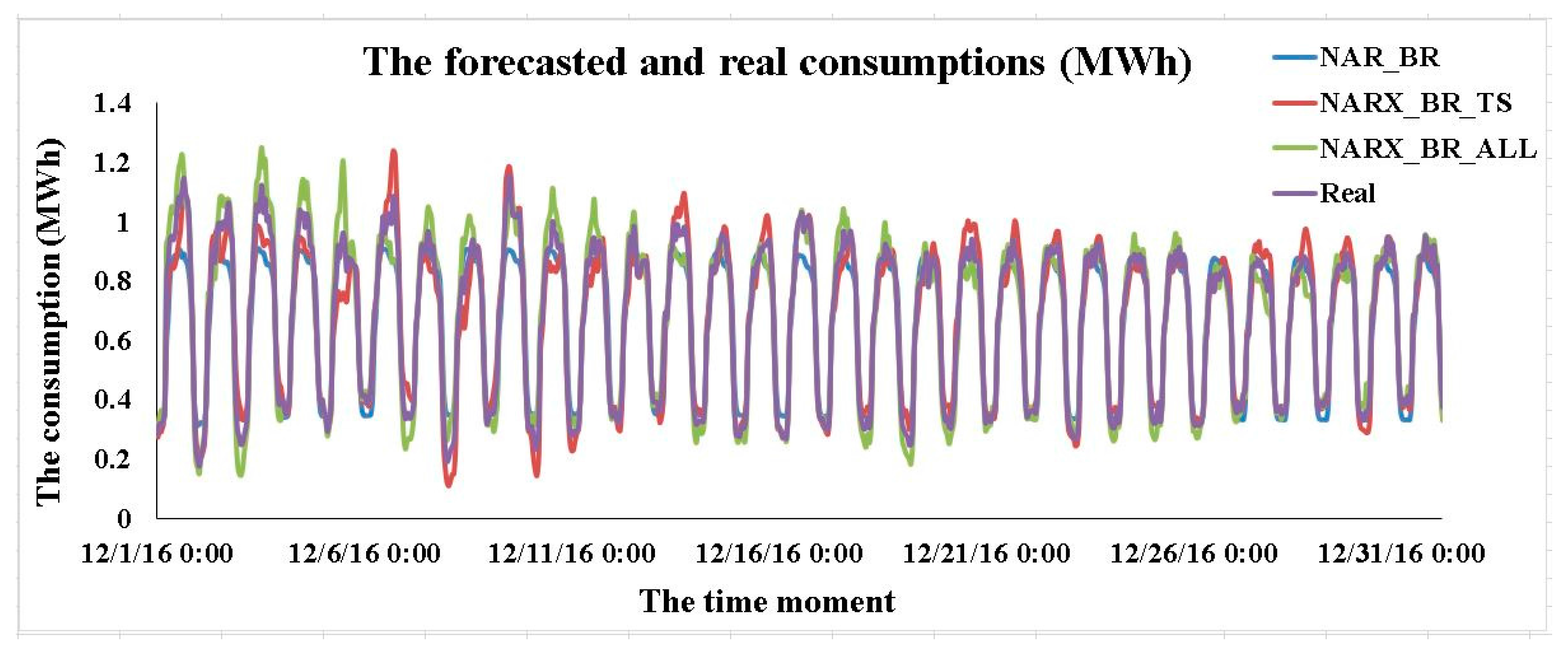
| 1 | ANN_NAR_BR | 0.00048272 | 0.99526 |
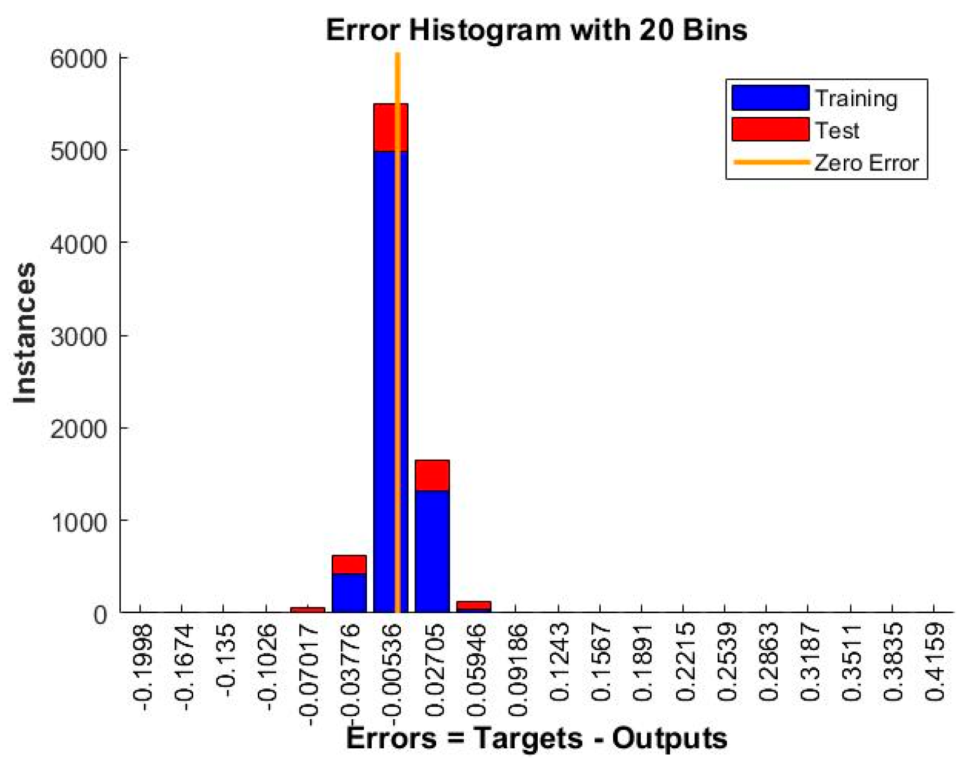
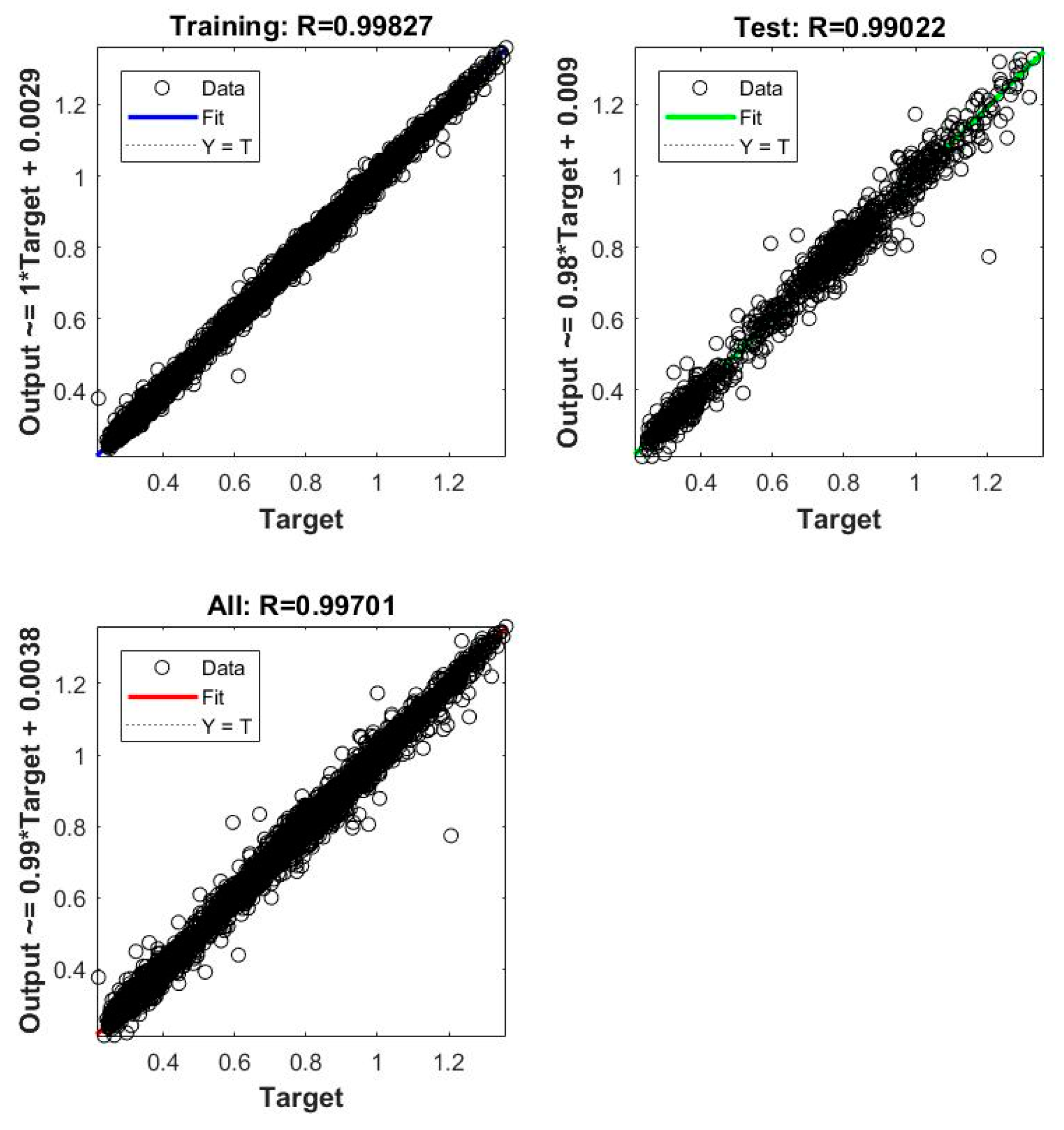
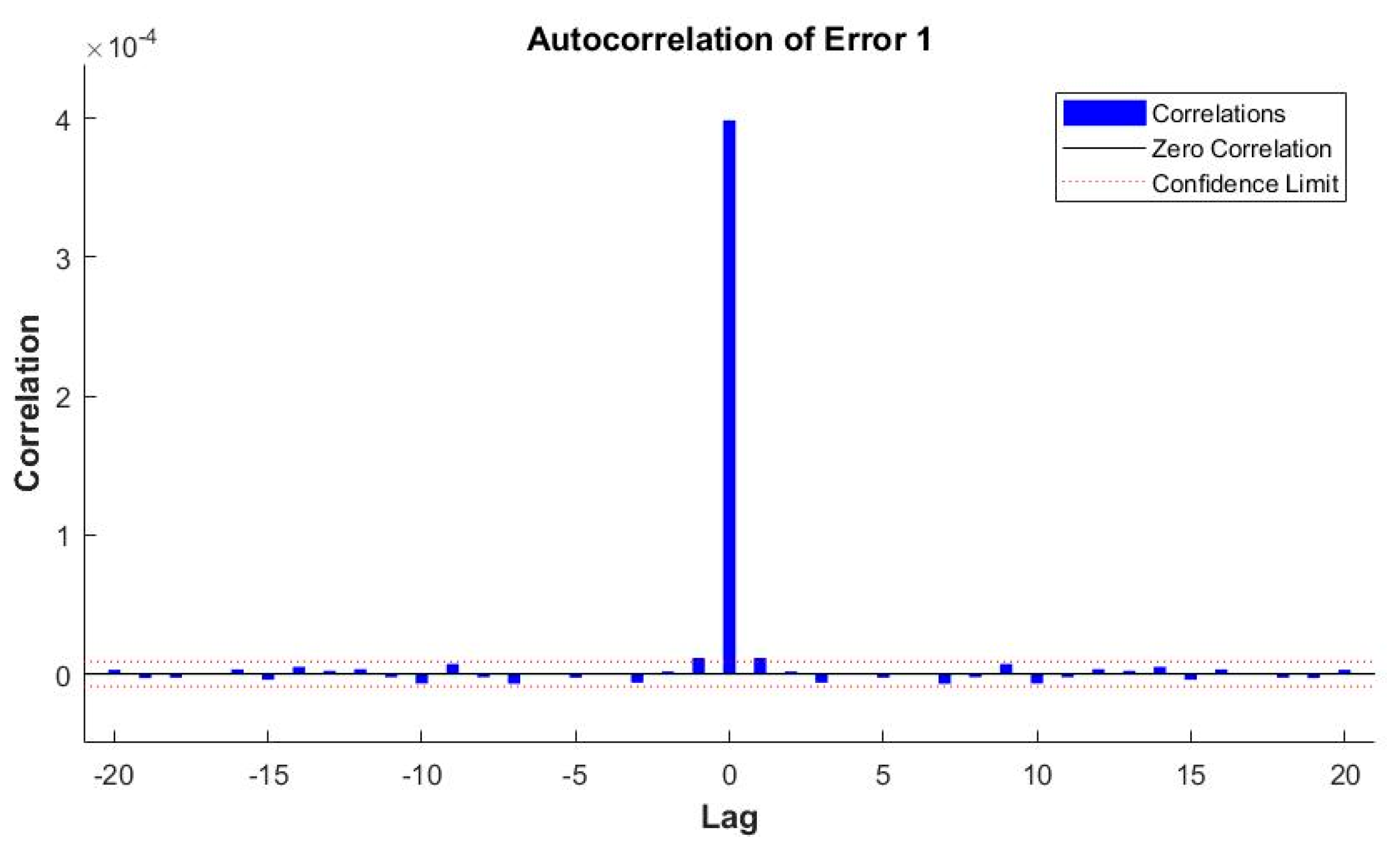
| 2 | ANN_NARX_BR_ALL | 0.0002294 | 0.99701 |
| 3 | ANN_NARX_BR_TS | 0.00032274 | 0.99623 |
| The Training Algorithm | The Model | ||
|---|---|---|---|
| NAR | NARX with Meteorological and Timestamps Exogenous Data | NARX with Timestamps Exogenous Data | |
| LM | , | , | , |
| BR | , | , | , |
| SCG | , | , | , |
| The Training Algorithm | The Model | ||
|---|---|---|---|
| NAR | NARX with Meteorological and Timestamps Exogenous Data | NARX with Timestamps Exogenous Data | |
| LM | | | |
| BR | | | |
| SCG | | | |
| The Training Algorithm | The Model | ||
|---|---|---|---|
| NAR | NARX with Meteorological and Timestamps Exogenous Data | NARX with Timestamps Exogenous Data | |
| LM | 75.33% for the MSE 1.83% for R | 41.66% for the MSE 0.37% for R | 61.57% for the MSE 0.23% for R |
| BR | 83.71% for the MSE 1.86% for R | 82.85% for the MSE 0.85% for R | 79.97% for the MSE 0.82% for R |
| SCG | 84.18% for the MSE 2.25% for R | 77.92% for the MSE 1.48% for R | 78.31% for the MSE 1.61% for R |
© 2017 by the authors. Licensee MDPI, Basel, Switzerland. This article is an open access article distributed under the terms and conditions of the Creative Commons Attribution (CC BY) license (http://creativecommons.org/licenses/by/4.0/).
Share and Cite
Pîrjan, A.; Oprea, S.-V.; Căruțașu, G.; Petroșanu, D.-M.; Bâra, A.; Coculescu, C. Devising Hourly Forecasting Solutions Regarding Electricity Consumption in the Case of Commercial Center Type Consumers. Energies 2017, 10, 1727. https://doi.org/10.3390/en10111727
Pîrjan A, Oprea S-V, Căruțașu G, Petroșanu D-M, Bâra A, Coculescu C. Devising Hourly Forecasting Solutions Regarding Electricity Consumption in the Case of Commercial Center Type Consumers. Energies. 2017; 10(11):1727. https://doi.org/10.3390/en10111727
Chicago/Turabian StylePîrjan, Alexandru, Simona-Vasilica Oprea, George Căruțașu, Dana-Mihaela Petroșanu, Adela Bâra, and Cristina Coculescu. 2017. "Devising Hourly Forecasting Solutions Regarding Electricity Consumption in the Case of Commercial Center Type Consumers" Energies 10, no. 11: 1727. https://doi.org/10.3390/en10111727