Controllability and Leader-Based Feedback for Tracking the Synchronization of a Linear-Switched Reluctance Machine Network


1
College of Mechatronics and Control Engineering, Shenzhen University, Shenzhen 518060, China
2
Laboratory of Advanced Unmanned Systems Technology, Research Institute of Northwestern Polytechnical University in Shenzhen, Shenzhen 518060, China
*
Authors to whom correspondence should be addressed.
Energies 2017, 10(11), 1728; https://doi.org/10.3390/en10111728
Submission received: 28 September 2017
/
Revised: 14 October 2017
/
Accepted: 24 October 2017
/
Published: 27 October 2017
(This article belongs to the Special Issue Networked and Distributed Control Systems)
Abstract
:This paper investigates the controllability of a closed-loop tracking synchronization network based on multiple linear-switched reluctance machines (LSRMs). The LSRM network is constructed from a global closed-loop manner, and the closed loop only replies to the input and output information from the leader node. Then, each local LSRM node is modeled as a general second-order system, and the model parameters are derived by the online system identification method based on the least square method. Next, to guarantee the LSRM network’s controllability condition, a theorem is deduced that clarifies the relationship among the LSRM network’s controllability, the graph controllability of the network and the controllability of the node dynamics. A state feedback control strategy with the state observer located on the leader is then proposed to improve the tracking performance of the LSRM network. Last, both the simulation and experiment results prove the effectiveness of the network controller design scheme and the results also verify that the leader-based global feedback strategy not only improves the tracking performance but also enhances the synchronization accuracy of the LSRM network experimentally.
1. Introduction
Tracking synchronization for electric machines can be vastly found in the manufacturing or assembly industries. There are many applications that require multiple linear machines to work in a coordinated manner [1]. For example, for a multiple linear-machine-based processing line, there are four working procedures such as drilling, welding, screwing and painting [2]. Each task is required to be accomplished by the corresponding linear machine regarding the procedure and the linear machines are expected to work cooperatively instead of sequentially. The piece of work being processed demands that the linear machines track the command position precisely and coordinate with each other to finish the entire work. Compared to the traditional sequenced working manner, the coordinated manner has the advantages of a faster operation time, more efficiency and the annihilation of accumulated errors, etc. [3].
Tracking synchronization networks based on linear switched reluctance motors (LSRM) are investigated in [2,3,4]. The LSRMs have the characteristics of simple and stable mechanical structures. Since no permanent magnet is involved, the cost of the machines is low with high reliability. They are more suitable for the construction of tracking networks on a large scale than the linear synchronous permanent magnet machines counterpart.
In a multiple linear-machine-based synchronization network, each linear machine can be regarded as a multi-agent and the coordinated control of the linear machines can be deemed as the design of consensus algorithms [5]. Analysis of the coordinated control of multi-agent networks provides a theoretical guidance for the construction and motion control of the LSRM network [6]. Consensus algorithms have been attempted in the areas of spacecraft clusters [7], mechanical systems coordination [8], and unmanned aerial vehicle formation [9], etc., with the implementation of robust consensus and self-adaptive algorithms. At present, consensus protocol studies can be categorized as covering the following aspects, such as nonlinear agent dynamics [9], constrained or imperfect communication [10], and the influence of noise [11], etc.
It can be concluded from the above analysis that the current theoretical work mainly concentrates on the connections between network stability, the control methods of the distributed network, and analysis of the network topology. The ultimate goal is to form a cohesion effect among the multiple agents within the network by the introduction of consensus algorithms. In addition, the aforementioned distributed control strategies only realize stable feedback control of the agents locally. However, from the network level, the tracking control for the reference signal is an “open loop”, which means that the entire network is constructed based on a global feed-forward control structure [12]. For an LSRM network, there are only local feedback loops on the leader machines, only accessing the reference information. Therefore, there is no feedback linkage to the entire network globally. As a result, the entire tracking control performance of the multiple LSRM networks is expected to be worse compared to the single LSRM-based tracking systems, since they are implemented based on a closed loop manner. It is natural that the global feedback strategy should be developed on the LSRM network for the improvement of tracking performance. Meanwhile, before any proper design of a network controller in a closed loop manner, the controllability of the LSRM network should first be guaranteed.
The main research objectives of network controllability are to seek the interrelationship between the network topological characteristics and the assignment of all nodes (or leaders) in order to ensure the network is fully controllable. Liu [13] proposes a mathematical tool based on the structure controllability theory of linear systems, and the method is successfully applied to analyze the controllability of a directed complex network and identify the minimum node sets of the network. Aiming at any complex network with arbitrary structures and known link–weight distributions, an exact controllability paradigm based on the maximum multiplicity is introduced to identify the minimum set of nodes that are required to achieve full controllability of the network [14]. Due to the non-uniqueness case of the minimum node sets of some controllability networks, the centrality measure quantifying a node’s likelihood of being a node is presented. In addition, the random sampling algorithm is applied to assess the quantity of the likelihood, in order to seek out the minimum node set with maximal efficiency [15]. A fundamental structure including source nodes, external dilation points and internal dilation points is discovered to elucidate the correlation between the network topology and the control properties. Furthermore, a control profile that quantifies the different proportions of control-inducing structures in a network is also developed for full controllability of a complex network [16]. Liu [17] further realizes the theoretical unity between the duality property of controllability and observability of complex networks and the dual principle of linear systems. Based on the determination of controllable and observable subspaces under the global minimum cost criterion, a domination centrality is employed to assess the node intervention capability, associated with the ability to dominate (control or observe) the state of other nodes in a directed network [18]. As a subcategory of network controllability, for the multi-agent network cohering through a consensus algorithm, the relationship between the network topology structure and the controllability of the network with a single leader is discussed, and some of the key results in this area are summarized [19].
We can conclude from the above-mentioned analysis that current research progress mainly concentrates on the connections between the network controllability and the network topology with leader(s) modeled as a graph only, which can be termed as graph controllability [20]. Moreover, the research on graph controllability is based on the hypothesis that the node dynamics are modeled as a single integrator. An LSRM network is not capable of a precise description of the complex and dynamic behavior of LSRMs if they are modeled as single integrator dynamics. As a result, if the LSRMs are modeled as general dynamics, the controllability of an LSRM node should be first considered. Therefore, when the LSRM network controllability is discussed for the design of the network feedback controller, the coupling influence caused by the controllability of each LSRM dynamic should not be neglected. In addition, because the consensus protocol algorithm contributes to the cohesion mechanism of the LSRM network, the properties of the consensus algorithm are certain to potentially affect the LSRM network controllability as well. To be specific, the LSRM network controllability is related to the graph controllability of the network and the controllability of the LSRM local closed-loop systems. According to the current literature, there are no generalized and practical conclusions available, considering the effect all of the above four factors [20].
In this paper, the mathematic model of the LSRM node is derived by online system identification based on the least square method. Therefore, each LSRM node is depicted as a general second-order system, instead of first-order dynamics. Then the standard second-order consensus control algorithm is employed to construct the LSRM network. Next, the condition that guarantees the LSRM network’s controllability is derived by presenting a theorem that elucidates the correlation between the LSRM network’s controllability and the graph controllability of the network and the controllability of the LSRM local closed-loop systems. Then, a state feedback control strategy is proposed and the state observer is located on the leader. The global closed loop manner improves the tracking performance of the entire LSRM network. Last, both the simulation and experiment verification is provided to prove the effectiveness of the network controller design scheme.
The contribution of this paper is twofold. Based on the global closed loop manner for the LSRM network, the authors first develop a theoretical support to ensure the controllability of the entire LSRM network, by analyzing the relationship from the LSRM network controllability to the LSRM node and graph controllability, respectively. Then, a feedback loop is constructed for the leader node to ensure that the entire LSRM network can track the given position reference signal more accurately.
2. Background Theory
2.1. Mathematical Model of the LSRM Node
Any of the three-phase LSRMs from the i-th node can be described in the voltage equation as [21],
where , and are terminal voltage, coil resistance and current; and represents the flux-linkage for the k-th winding. The LSRM can also be depicted as the second-order dynamics as,
where , , , and represent position, friction coefficient, mass, total and load force for the i-th LSRM, respectively. The second-order system can be further represented in the discrete-time form as [22],
where and are polynomials to be determined and denotes unknown disturbances for the i-th LSRM node. Polynomial and correspond to a typical discrete-time form as,
The purpose of online system identification is to correctly estimate , , and that contain all dynamic information. For the n-th estimation, Equation (3) can also be considered as a typical least square form as,
where,
The parameters described in the above equation can be estimated by the recursive least square method as [23],
Stochastic errors can be represented as,
where the symbol means the estimated variable vector; is the covariance matrix; and is the gain. is the forgetting factor that reflects the relationship between the converging rate and tracking ability and it falls into 0 and 1. For the LSRM nodes, is chosen as 0.98 for moderate converging ripples and fast identification speed. For initial values, can be chosen as with as a constant value of 50 and is a four-dimension unit matrix. If the relative error from the present to the last step is comparatively a small value , it can be regarded that the present estimated value is correct [24]. Then the criterion to terminate the program for the recursive calculation can be set as,
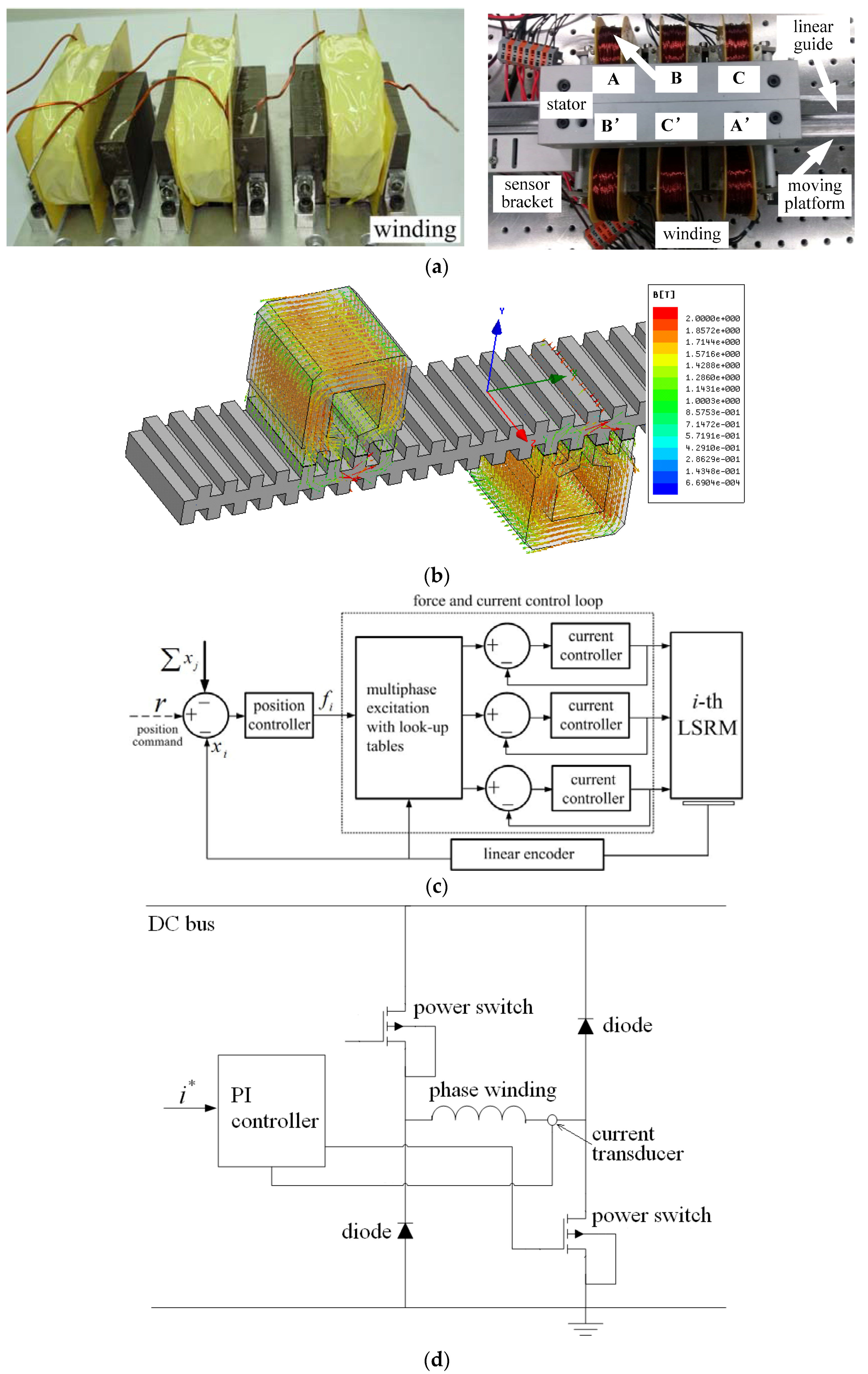
Figure 1a is the winding and the LSRM picture. Figure 1b is the flux contour from the finite element analysis for any one phase and it clear that each phase can be controlled independently [4]. The control block diagram for any LSRM node can be depicted as shown in Figure 1c. The i-th LSRM node receives both the position feedback information from its linear encoder and the j-th node and only the leader node accesses the position reference information. Each node is composed of a local position controller, the multiphase excitation scheme with look-up table linearization, current controllers to form the force and current control loop, and an LSRM [22]. For the i-th LSRM node, error is decided from the difference between reference (the leader only) and actual position xi of the i-th LSRM, along with the position information from the j-th LSRM xj. The position controller then calculates the control input and the multi-phase excitation with a look-up table linearization scheme determines the current command for the k-th phase, according to the current position of the i-th LSRM. Then the current controller outputs the actual current to the k-th winding. Figure 1d is the power electronics drive topology.
2.2. Second-Order Consensus Algorithm and LSRM Network Dynamics
Rearranging Equation (2) in the state-space form, we have,
where . The standard second-order consensus algorithm [25] is applied to design the coordinated control law for the LSRM network. It is formulated as,
where is the entry of adjacency matrix associated with graph . The velocity feedback terms and are obtained by the differential of position and from the position control loop and are the position and velocity gains. The dynamic equation for the i-th LSRM node can thus be represented as,
The dynamic equation for the LSRM network can thus be derived as,
where is the N-th identity matrix and is the Laplacian matrix. Let , , , .
Since all the LSRM nodes are identical according to Assumption 1, as follows, all the subscripts for can be neglected. Therefore, the above equation can be represented as,
The following assumptions are made to limit the scope of the study in accordance with the actual characteristics of the LSRM network:
Assumption 1.
There is a sole LSRM as the leader for controlling and observing the LSRM network and each LSRM node is considered identical.
Assumption 2.
The network topology is modeled as an undirected graph, that is, the existent communication of any two LSRMs is bidirectional.
3. Controllability Analysis of LSRM Network
3.1. Input-Output of Network
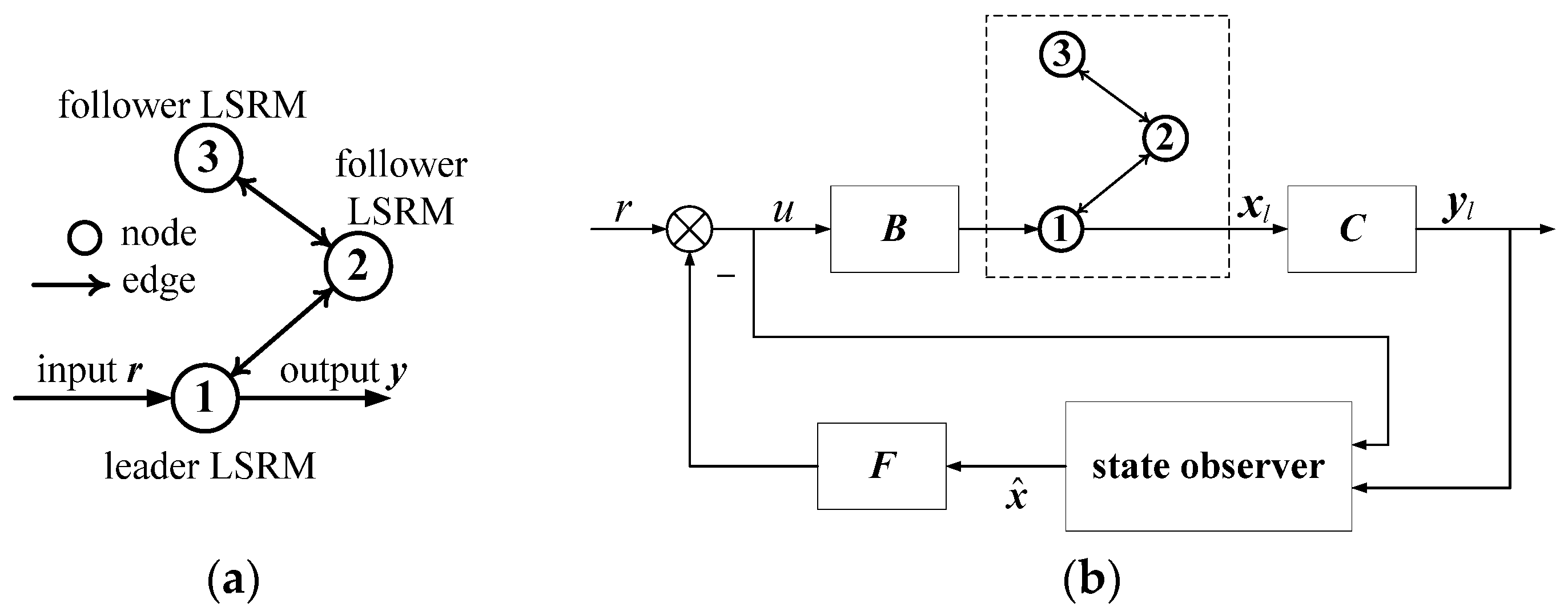
Under Assumptions 1 and 2, the communication topology of the LSRM network is indicated by Figure 2a, and the LSRM nodes of the network with bidirectional communication can be classified as the single leader node and the follower nodes, respectively. is the global feedback tracking controller.
Since the leader node is driven by the external reference signal as the control input of the LSRM network and the state of the leader is observed as the output of the LSRM network, the open-loop dynamics can be expressed as,
The state and output of the leader is denoted as and , respectively. is the output matrix of the LSRM node. The follower nodes are only driven by the leader node internally from the network. Therefore, the dynamics of the follower nodes can be represented as,
Here, the state of the follower nodes is denoted by . By combining Equation (15) with Equation (16), the dynamics of the LSRM network with input and output can be expressed as,
where . is the output of the LSRM network.
3.2. Controllability and Observability of LSRM Network
For the design of the state feedback control based on the input and output of the leader, the controllability and observability of the LSRM network should be guaranteed by selecting an eligible leader node for the network. The controllability of the LSRM network can be formulated by the controllability of Equation (17), i.e., to ensure that system matrix and input matrix of the LSRM network are a controllable matrix pair.
Definition 1.
Graph controllability can be described as when the network composed of and is controllable, that is to say, and form a controllable matrix pair.
To facilitate the representation of derivation, the first formula in Equation (17) is rewritten as,
where is the input signal outside the LSRM network, and the function is the same as in Figure 1. In addition, the system matrix and input matrix are as follows,
According to Definition 1 and [23], the prerequisite for using some external signal to manipulate freely the LSRM network Equation (18) is that its controllability can be guaranteed.
3.3. Controllability of LSRM Network
A sufficient and necessary condition for the controllability of the LSRM network Equation (18) is presented in the following theorem.
Theorem 1.
The controllability of the LSRM network represented as is identical as the graph controllability (the controllability of the coordinated network) described as , if associated with the LSRM nodes i are all controllable.
Proof of Theorem 1.
Let and denote an eigenvalue and its corresponding left eigenvector of matrix , respectively. The equation can be written as,
☐
Let , here is the left eigenvector of Laplacian matrix that satisfies the following equation,
Therefore, Equation (20) can be rewritten as,
where the right side of Equation (22) satisfies the following,
Meanwhile, by applying Equation (21) and the Kronecker product properties, the left side of Equation (22) can be derived as follows,
According to Equations (22)–(24), we can derive the equation as,
By applying Equation (12), we can derive the following equation as,
According to Equations (25) and (26), the characteristic polynomial of Equation (26) is obtained as,
Therefore, the eigenvalues of the matrix Equation (26) can be derived as,
Subsequently, substituting Equation (26) into Equation (25), we can derive the following equation,
where . From Equation (29), the following equation is derived,
If is satisfied for Equation (28), the two eigenvectors and in Equation (30) associated to and in Equation (28) can be solved as,
According to the Popov–Belevitch–Hautus (PBH) controllability criteria [23], the LSRM network’s is controllable if and only if the following equations is satisfied.
Here all can be represented as,
here i can be divided into two cases that j > 0 and,
According to Equation (33), the following equation can be derived,
By Equation (33), we note is held if and only if and . If is held, from Equations (34) and (25), we have,
That is to say, the i-th local closed-loop LSRM system is controllable. Obviously, as long as , in Equation (32), Equation (34) can be satisfied. That is to say, combining with Equation (21), Equation (32) is held if and only if the following equation can be satisfied,
Equation (36) indicates that the coordinated network is controllable. Theorem 1 is proved.
Remark 1.
According to Theorem 1, the controllability of an LSRM network is fully decided by both graph controllability and the controllability of all local closed-loop LSRM systems.
Remark 2.
The result of Theorem 1 is understandable intuitively. The LSRM network can be regarded as a cascading control system with a higher networked control layer of coordinated network and a lower local closed-loop feedback layer of each LSRM node. The function of the lower layer is to control each LSRM system to track the command calculated through the coordinated control law, such as a consensus algorithm from the higher layer. Therefore, an LSRM network can be fully controlled by an external signal, in other words, an LSRM network is controllable only if the external signal can manipulate fully the entire coordinated network, and the network coupling signal formed by the network graph can steer each local LSRM system simultaneously.
Remark 3.
From Equation (35), we notice that the local LSRM system mentioned in Theorem 1 is not independent and unrelated. Instead, the i-th local LSRM system couples with the network graph by the i-th eigenvalue of Laplacian matrix .
Remark 4.
In Theorem 1, the proposed controllability criteria applied to the networked control system connected by general second-order dynamics nodes, such as the LSRM network, is more practical than the other methods mentioned by [26], since the criteria reveals clearly the relationship between the controllability of the network comprised of second-order nodes and the graph controllability of the network and the controllability of the node dynamics.
4. Output–Feedback Control Design
4.1. LSRM Network Control Design
To realize the closed loop control by utilizing the input and output information of the leader node, the following controller is presented [26],
where is the state estimation values from the observer and is the reference. The state observer can be depicted as,
where is the input estimation values from the observer and can be described as,
Substituting (39) into (38), we have,
The control block diagram of the LSRM network with the state observer can be depicted as shown in Figure 2b. The LSRM network dynamic can be represented as,
where
where
In addition, , and are the zero matrix with the dimensions of and , respectively. It can be deducted from (39) that the entire network dynamic is composed of both the closed loop equation of the LSRM network and the estimated error equation from the state observer.
4.2. Control Schemes for Leader and Follower
From (16), (37) and (40), we can derive the following control equations for the leader and followers,
From (23) for the states of the leader, the control function includes two parts. The first part is the consensus algorithm and the second is the closed loop control part . are the node sets which communicate bidirectionally with the leader and followers, individually. is derived by the solution of (44), which utilizes leader output and leader input to reconfigure the states of the entire LSRM network. The states of the followers are controlled by the consensus algorithm only, as depicted in (43). Therefore, the global closed control is successfully implemented by the input and output information of the leader only.
4.3. Solution of Controller Gain and Observer Gain Based on Pole-Placement
From the above analysis of controllability and observability, the suitable control laws can be developed to achieve desired eigenvalues (expected poles) for the controller and the observer. According to separation principle of linear systems, the eigenvalues of (41) can be represented as the unit set of
and
as follows,
Therefore, the solutions of the controller gain and the observer gain can be obtained independently. The desired eigenvalues of the controller and the observer can thus be derived from the pole placement method of linear system theory.
5. Experiment Verification
5.1. Network Configuration
The hardware frame of the LSRM network composed of three LSRMs is depicted in Figure 3. Communication between the LSRM nodes is realized by the serial port with an RS232 protocol with a baud rate of 57,600 and the data and stop bit set are eight and one, respectively. “External signals” represent the neighbors’ position information and also the reference signal for LSRM node 1. “Internal signals” are the position information within the nodes.
5.2. Experiment Setup
Each LSRM node utilizes one dSPACE DS1104 board and can directly interface with MATLAB/SIMULINK by the virtual software ControlDesk® from dSPACE company in Germany. All the control parameters or state variables can be modified online and were saved as a standard data format for further processing. Each control board connects one linear encoder through the 24-bit incremental encoder channel and the communication among the LSRM nodes was realized by the serial port. The control objects are three identical LSRMs that conform to the “6/4” switched reluctance machine structure. A double-sided machine arrangement guarantees a more stable and reliable output performance and the asymmetry of the stators ensures a higher force-to-volume ratio [25]. Table 1 demonstrates the major specifications of the LSRM.
As shown in Figure 4, each LSRM node is composed of the LSRM, the power supply with transformers and the dSPACE control board and the connection interface. Current control is realized by three commercial amplifiers that are capable of inner current regulation of 20 kHz switching frequency based on the proportion integral algorithm, according to Figure 1c. The sampling frequency of the position control loop is 1 kHz.
5.3. Control Parameter Derivations
Table 2 tabulates the control and observer parameters. The LSRM parameters can be obtained as , , and , respectively, through the online recursive least square parameter identification scheme. The position and velocity gains of the local coordinated controller are selected based on a trial and error basis as 2 and 0.02, respectively. The expected poles of the controllers and the observer are selected to ensure a quick and precise dynamic response [26]. Then controller and observer gains can be calculated according to (45).
5.4. Tracking Performance Analysis
The experimental tracking response waveforms for the three LSRMs without leader-based feedback can be found in Figure 5. According to the tracking profiles of the three LSRMs in Figure 5a, the LSRMs are all capable of following the position reference signal.
However, the control performance from the three LSRMs is not uniform, especially at the time interval of (40 s, 50 s). This is mainly because the imperfect manufacture and assembly of the leader LSRM1, which results in asymmetric control performance from the positive and negative transitions, especially as the machine approaches to the motion limit [25]. The tracking response of LSRM1 is the reference signal of LSRM2 and LSRM3 and the position response is further propagated through the communication link to LSRM2 and LSRM3. Since the communication is bidirectional, the position response from LSRM2 and 3 can even be transmitted back to LSRM1. Therefore the control performance for the three LSRM nodes is further deteriorated and exhibits local oscillations from the tracking profiles, which can be further clarified by Figure 5b. The error response profiles of each LSRM to the reference signal demonstrate higher frequency characteristics. The maximum dynamic error values of the LSRMs to the reference signal fall into ±5 mm. Figure 5c is the relative error response between any two LSRMs and it illustrates the consensus performance of the LSRM network. After about 3 s of regulations, the relative error values fall into ±4 mm for LSRM1 to LSRM2 and LSRM1 to LSRM3. Since the leader LSRM1 is affected by the reference signal, it acts as an external disturbance both to the consensus from LSRM1 to LSRM2 and from LSRM1 to LSRM2. As a result, the error waveforms demonstrate a pseudo-periodical response according to the frequency of the reference signal. The error waveforms from LSRM2 and LSRM3 do not exhibit the frequency characteristics of the reference signal, since the consensus is not directly influenced by the reference according to the communication topology. It can be concluded that the error performance between LSRM2 and LSRM3 is more dominated by the consensus algorithm since the error mean value is about zero.
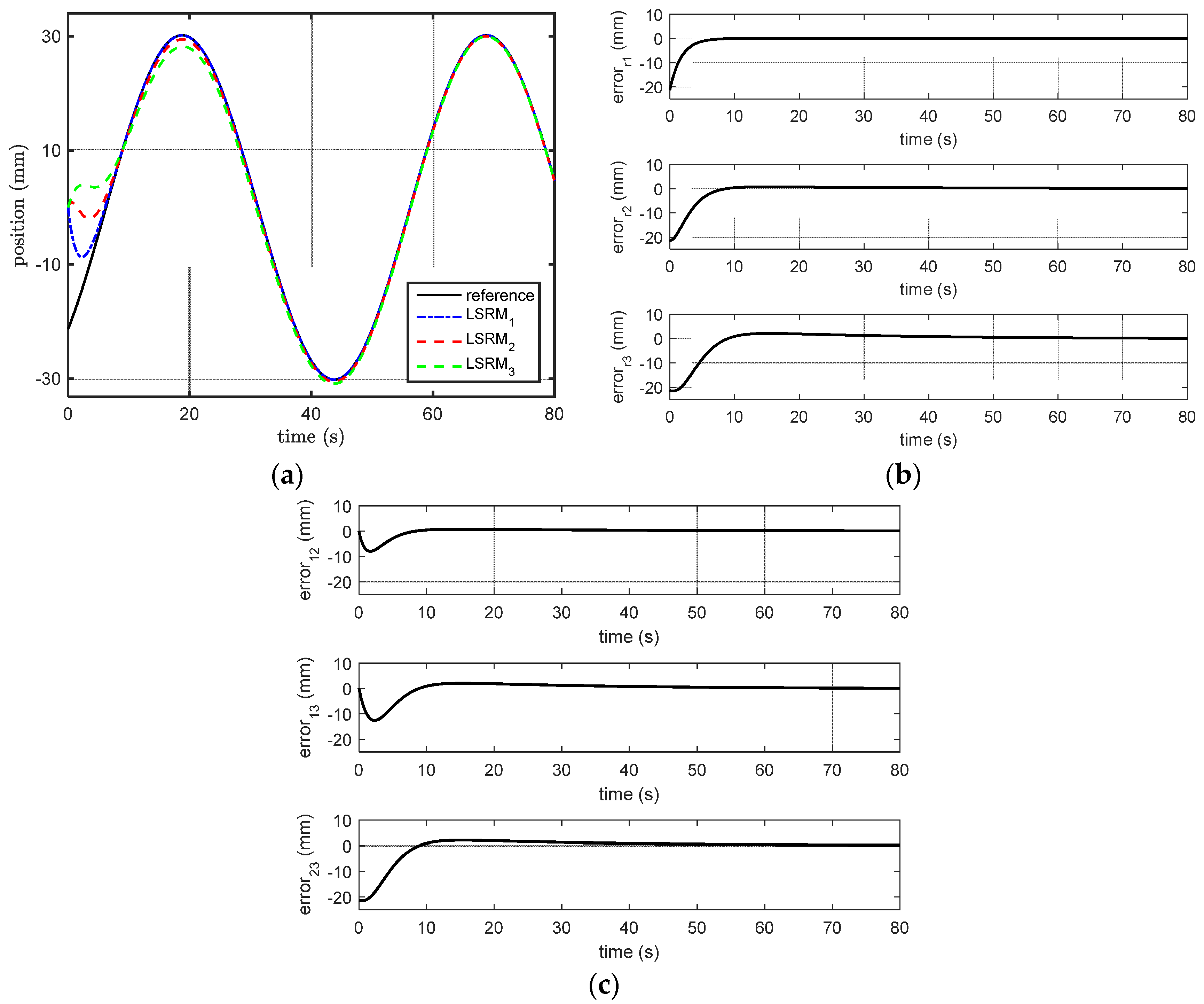
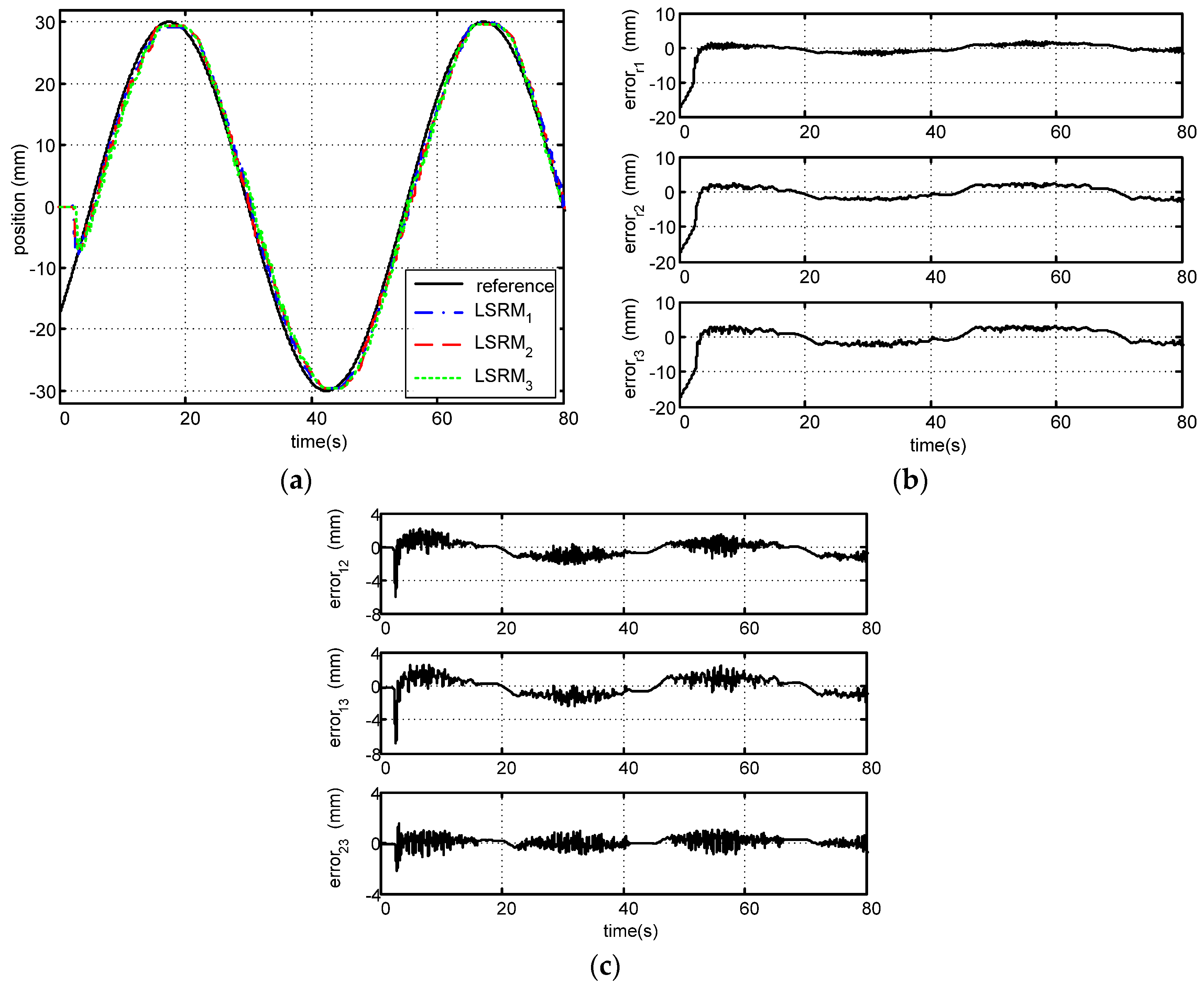
The simulation results of the tracking profiles from the three LSRMs and error response with the lead-based feedback can be found in Figure 6. It can be concluded that the LSRMs can quickly and effectively follow the reference signal. The steady-state error for each machine ideally falls into zero. The tracking profiles of the three LSRMs and error response with the lead-based feedback can be found in Figure 7. The results correspond to those from the simulation. Due to mechanical restraints from the LSRMs, such as mass and inertia, and the limited response speed from the power drives, the settling time and the comparatively low and steady-state error values cannot reach zero.
From Figure 7a, it is clear that the response waveforms are nearly uniform for either positive or negative transitions according to the reference signal. It can also be seen that the high-frequency oscillations from the negative response transition are reduced. Since the performance of the leader LSRM1 is effectively improved by the closed loop control manner based on the feedback of the entire LSRM network, the tracking error for each LSRM node to the reference can be further reduced, as shown in Figure 7b. From Figure 7c, it can be seen that the synchronization performance is also improved under the leader-based feedback strategy, with maximum dynamic error values falling into ±1.5 mm. It can be concluded that the global leader-based feedback strategy not only improves the tracking performance but also enhances the synchronization accuracy of all LSRM nodes.
6. Conclusions and Discussion
A leader-based, closed loop network tracking control strategy is proposed in this paper. The dynamic behavior of the LSRM nodes were modeled as general second-order linear systems by online system identification. The condition for the LSRM network’s controllability was guaranteed by the derivation of the theorem, which considers the relationship between the LSRM network controllability and the graph controllability of the network and the controllability of the node dynamics. A state feedback control strategy with the state observer by utilizing the input and output of the leader was implemented to improve the tracking performance of the entire LSRM network. The experiment results verifid that the global leader-based feedback control not only improved the tracking performance but also enhanced the synchronization accuracy of the entire LSRM network. The proposed scheme can be applied to electric machine-based motion control networks, such as in the industrial automation field of automobile assembly process, etc.
Due to the limitations from the mass and the inertia of the local LSRMs and the network hardware interface, the proposed global control strategy is suitable for the coordination of low-speed, reciprocal linear translations with lower dynamics experimentally. To further improve the tracking precision, it is suggested that the internal model compensation scheme is introduced to the feedback control design of the LSRM network. For the tracking of periodical sinusoidal reference signals, frequency domain analysis is also recommended for better configuration of the expected poles. Furthermore, detailed study on load influence for different local systems will be carried out.
The LSRM network was constructed based on individual dSPACE control boards. The manner of the serial port communication may influence the precision of the network if packet dropouts or delays occur. Future research will focus on the implementation of three digital, single-chip processors to further improve the precision of the LSRM network.
Acknowledgments
This work was supported in part by the National Natural Science Foundation of China under Grant Nos. 51477103, 51577121, 11572248, 61690211 and 61403258. The authors also would like to thank the Guangdong and Shenzhen Governments under the Code of S2014A030313564, 2015A010106017, 2016KZDXM007, JCYJ20160308104825040 and JCYJ20170302145012329 for support.
Author Contributions
Bo Zhang and Jianping Yuan conceived and wrote the main body of the paper, and Jianfei Pan designed the main body of study. Li Qiu guided the system design, analyzed the data and revised the manuscript. Xiaoyu Wu performed the simulations and experiments. Jianjun Luo and helped to revise the paper.
Conflicts of Interest
The authors declare no conflict of interest.
References
- Leitao, P.; Marik, V.; Vrba, P. Past, Present, and future of industrial agent applications. IEEE Trans. Ind. Inf. 2013, 9, 2360–2372. [Google Scholar] [CrossRef]
- Zhang, B.; Yuan, J.; Luo, J.; Wu, X.; Qiu, L.; Pan, J.F. Hierarchical distributed motion control for multiple linear switched reluctance machines. Energies 2017, 10, 1426. [Google Scholar] [CrossRef]
- Zhang, B.; Pan, J.F.; Yuan, J.; Rao, W.; Qiu, L.; Luo, J.; Dai, H. Tracking control with zero phase-difference for linear switched reluctance machines network. Energies 2017, 10, 949. [Google Scholar] [CrossRef]
- Zhang, B.; Yuan, J.; Qiu, L.; Cheung, N.; Pan, J.F. Distributed coordinated motion tracking of the linear switched reluctance machine-based group control system. IEEE Trans. Ind. Electron. 2016, 63, 1480–1489. [Google Scholar] [CrossRef]
- Olfati-Saber, R.; Fax, J.A.; Murray, R.M. Consensus and cooperation in networked multi-agent systems. Proc. IEEE 2007, 95, 215–233. [Google Scholar] [CrossRef]
- Yu, W.; Chen, G.; Cao, M.; Ren, W. Delay-induced consensus and quasi-consensus in multi-agent dynamical systems. IEEE Trans. Circuits Syst. I 2013, 60, 2679–2687. [Google Scholar] [CrossRef]
- Ma, C.; Shi, P.; Zhao, X.; Zeng, Q. Consensus of Euler–Lagrange systems networked by sampled-data information with probabilistic time delays. IEEE Trans. Cybern. 2015, 45, 1126–1133. [Google Scholar] [PubMed]
- Wang, H. Consensus of networked mechanical systems with communication delays: A unified framework. IEEE Trans. Autom. Control 2014, 59, 1571–1576. [Google Scholar] [CrossRef]
- Cao, Y.; Yu, W.; Ren, W.; Chen, G. An overview of recent progress in the study of distributed multi-agent coordination. IEEE Trans. Ind. Inf. 2012, 9, 427–438. [Google Scholar] [CrossRef]
- Li, L.; Ho, D.W.C.; Lu, J. A unified approach to practical consensus with quantized data and time delay. IEEE Trans. Circuits Syst. I 2013, 60, 2668–2678. [Google Scholar] [CrossRef]
- Wei, J.; Fang, H. Multi-agent consensus with time-varying delays and switching topologies. J. Syst. Eng. Electron. 2014, 25, 489–495. [Google Scholar] [CrossRef]
- Dong, X.; Yu, B.; Shi, Z.; Zhong, Y. Time-varying formation control for unmanned aerial vehicles: Theories and Applications. IEEE Trans. Control Syst. Technol. 2014, 23, 340–348. [Google Scholar] [CrossRef]
- Liu, Y.; Slotine, J.E.; Barabasi, A. Controllability of complex networks. Nature 2011, 473, 167–173. [Google Scholar] [CrossRef] [PubMed]
- Yuan, Z.; Zhao, C.; Di, Z.; Wang, W.; Lai, Y. Exact controllability of complex networks. Nat. Commun. 2013, 4, 2447. [Google Scholar] [CrossRef] [PubMed]
- Jia, T.; Barabasi, A. Control Capacity and A random sampling method in exploring controllability of complex networks. Sci. Rep. 2013, 3, 2354. [Google Scholar] [CrossRef] [PubMed]
- Ruths, J.; Ruths, D. Control profiles of complex networks. Science 2014, 343, 1373–1376. [Google Scholar] [CrossRef] [PubMed]
- Liu, Y.; Slotine, J.E.; Barabasi, A. Observability of complex systems. Proc. Natl. Acad. Sci. USA 2013, 110, 2460–2465. [Google Scholar] [CrossRef] [PubMed]
- Wang, B.; Gao, L.; Gao, Y.; Deng, Y.; Wang, Y. Controllability and observability analysis for vertex domination centrality in directed networks. Sci. Rep. 2014, 4, 5399. [Google Scholar] [CrossRef] [PubMed]
- Egerstedt, M.; Martini, S.; Cao, M.; Camlibel, K.; Bicchi, A. Interacting with networks: How does structure relate to controllability in single-leader, consensus networks? IEEE Control Syst. Mag. 2012, 32, 66–73. [Google Scholar] [CrossRef]
- Cai, N.; Cao, J.; Khan, M.J. A Controllability synthesis problem for dynamic multi-agent systems with linear high-order protocol. Int. J. Control Autom. Syst. 2014, 12, 1366–1371. [Google Scholar] [CrossRef]
- Qiu, L.; Shi, Y.; Pan, J.; Zhang, B.; Xu, G. Collaborative tracking control of dual linear switched reluctance machines over communication network with time delays. IEEE Trans. Cybern. 2016, 1–11. [Google Scholar] [CrossRef] [PubMed]
- Lu, F.; Ye, Y.; Huang, J. Gas turbine engine identification based on a bank of self-tuning wiener models using fast kernel extreme learning machine. Energies 2017, 10, 1363. [Google Scholar] [CrossRef]
- Rahimi-Eichi, H.; Baronti, F.; Chow, M. Online adaptive parameter identification and state-of-charge coestimation for lithium-polymer battery cells. IEEE Trans. Ind. Electron. 2014, 61, 2053–2061. [Google Scholar] [CrossRef]
- Deng, Z.; Yang, L.; Cai, Y.; Deng, H. Online identification with reliability criterion and state of charge estimation based on a fuzzy adaptive extended Kalman filter for lithium-ion batteries. Energies 2016, 9, 472. [Google Scholar] [CrossRef]
- Wang, L.; Chen, G.; Wang, X.; Tang, W.K.S. Controllability of networked MIMO systems. Automatica 2016, 69, 405–409. [Google Scholar] [CrossRef]
- Astrom, K.J.; Murray, R.M. Feedback Systems: An Introduction for Scientists and Engineers; Princeton University Press: Princeton, NJ, USA, 2008. [Google Scholar]
Figure 1.
(a) The linear switched reluctance machine prototype; (b) finite element analysis of flux; (c) block diagram for a single LSRM node; and (d) power electronic drive circuit.
Figure 1.
(a) The linear switched reluctance machine prototype; (b) finite element analysis of flux; (c) block diagram for a single LSRM node; and (d) power electronic drive circuit.

Figure 2.
(a) Network topology; (b) block diagram of the proposed control scheme.

Figure 3.
LSRM network hardware frame.
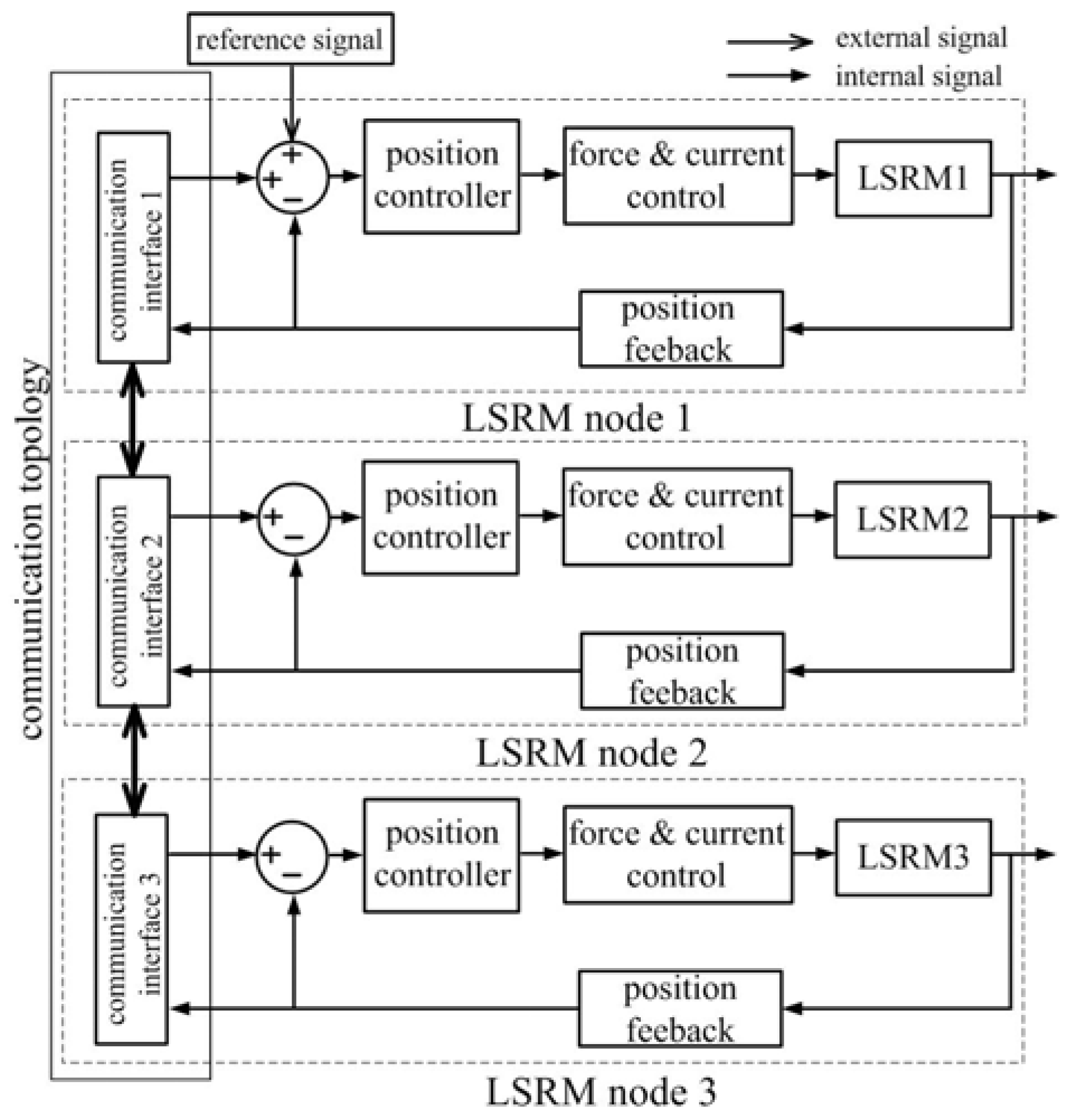
Figure 4.
Experiment setup.
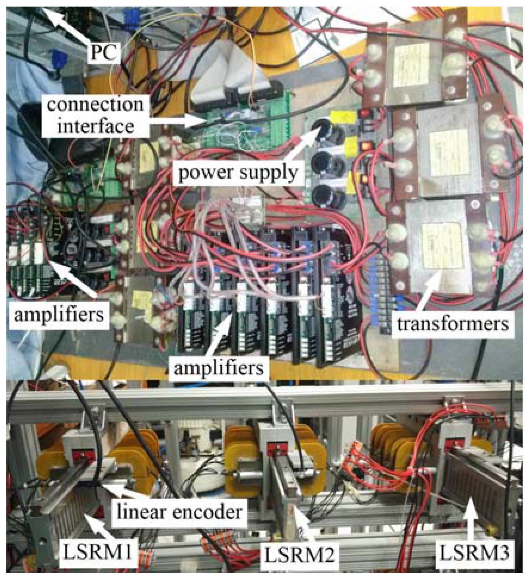
Figure 5.
Tracking profiles (a) LSRMs; (b) error response to reference; and (c) relative error response between LSRMs without leader-based feedback.
Figure 5.
Tracking profiles (a) LSRMs; (b) error response to reference; and (c) relative error response between LSRMs without leader-based feedback.

Figure 6.
Simulation results (a) LSRMs; (b) error response to reference; and (c) relative error response between LSRMs with leader-based feedback.
Figure 6.
Simulation results (a) LSRMs; (b) error response to reference; and (c) relative error response between LSRMs with leader-based feedback.

Figure 7.
Tracking profiles (a) LSRMs; (b) error response to reference; and (c) relative error response between LSRMs with leader-based feedback.
Figure 7.
Tracking profiles (a) LSRMs; (b) error response to reference; and (c) relative error response between LSRMs with leader-based feedback.


Table 1.
Major specifications.
| Parameter | Value |
|---|---|
| Mass of moving platform | 3.8 kg |
| Mass of stator | 5.0 kg |
| Pole width | 6 mm |
| Pole pitch | 12 mm |
| Phase resistance | 2 ohm |
| Air gap length | 0.3 mm |
| Number of turns | 200 |
| Stack length | 50 mm |
| Encoder resolution | 1 µm |
Table 2.
Expected poles, gain and parameters.
| Parameter | Controller | Observer |
|---|---|---|
| Expected poles | ||
| Gain | ||
| Control parameters |
© 2017 by the authors. Licensee MDPI, Basel, Switzerland. This article is an open access article distributed under the terms and conditions of the Creative Commons Attribution (CC BY) license (http://creativecommons.org/licenses/by/4.0/).
Share and Cite
MDPI and ACS Style
Zhang, B.; Yuan, J.; Pan, J.; Wu, X.; Luo, J.; Qiu, L. Controllability and Leader-Based Feedback for Tracking the Synchronization of a Linear-Switched Reluctance Machine Network. Energies 2017, 10, 1728. https://doi.org/10.3390/en10111728
AMA Style
Zhang B, Yuan J, Pan J, Wu X, Luo J, Qiu L. Controllability and Leader-Based Feedback for Tracking the Synchronization of a Linear-Switched Reluctance Machine Network. Energies. 2017; 10(11):1728. https://doi.org/10.3390/en10111728
Chicago/Turabian StyleZhang, Bo, Jianping Yuan, Jianfei Pan, Xiaoyu Wu, Jianjun Luo, and Li Qiu. 2017. "Controllability and Leader-Based Feedback for Tracking the Synchronization of a Linear-Switched Reluctance Machine Network" Energies 10, no. 11: 1728. https://doi.org/10.3390/en10111728
Note that from the first issue of 2016, this journal uses article numbers instead of page numbers. See further details here.