
Simulating Extreme Directional Wave Conditions


School of Engineering, Institute for Energy Systems, The University of Edinburgh, Edinburgh EH9 3DW, UK
*
Author to whom correspondence should be addressed.
Energies 2017, 10(11), 1731; https://doi.org/10.3390/en10111731
Submission received: 22 September 2017
/
Revised: 17 October 2017
/
Accepted: 24 October 2017
/
Published: 28 October 2017
(This article belongs to the Special Issue Marine Energy)
Abstract
:Wave tank tests often involve simulating extreme wave conditions as they enable the maximum expected loads to be inferred: a vital parameter for structural design. The definition, and simulation of, extreme conditions are often fairly simplistic, which can result in conditions and associated loads that are not representative of those that would be observed at the deployment location. Here we present a method of defining, simulating at scale, and validating realistic site-specific extreme wave conditions for survival testing of wave energy converters. Bivariate inverse-first order reliability method (I-FORM) environmental contours define extreme pairs of significant wave height and energy period (–), while observed extreme conditions are used to define realistic frequency and directional distributions. These sea states are scaled, simulated and validated at the FloWave Ocean Energy Research Facility to demonstrate that the site-specific extreme wave conditions can be re-created with accuracy. The presented approach enables greater realism to be incorporated into tank testing with survival sea states. The techniques outlined and explored here can provide further and more realistic insight into the response of offshore structures and devices, and can help make important design decisions prior to full-scale deployment.
1. Introduction
Offshore structures and devices, including wave energy converters (WECs), are tested in wave tanks to assess behaviour, performance and loads at scale prior to deployment at sea. For survivability, it is paramount to identify the expected extreme conditions, which often initially focusses on the identification of extreme significant wave heights. This is achieved using extreme value distributions to extrapolate the observed data to the desired return period and is suggested by Goda [1] to be the first step in coastal structure design. Extreme sea states are hence often used in such test programmes and enable the largest expected loads to be inferred, which can feed back into design and help validate numerical prediction.
When defining extreme wave conditions, it is common to extrapolate extreme significant wave height, , values as detailed in Coles [2], Caires [3], Teena et al. [4]. To define and simulate sea states, however, appropriate wave period values are also required. These can be obtained using joint probability methods such as the inverse-first order reliability method (I-FORM) technique (implemented in Haver and Nyhus [5], Winterstein et al. [6], Berg [7]) recommended by the EquiMar Protocols [8] for defining extreme conditions for WECs. These methods provide environmental contours relating to certain probabilities or return periods. The I-FORM method has been implemented in Doherty and Folley [9] to define extreme significant wave height–period (H–T) combinations for Aquamarine’s Oyster WEC, which is used a basis to create extreme wave spectra for tank testing. In this case, Bretschneider spectra were used in all cases, and it is assumed that they have been created without directional spreading. Despite a robust process to arrive at representative extreme H–T combinations, the resulting parametric sea states may differ significantly from those actually associated with extreme events at the site. Observed spectral shapes are often not well described by two-parameter spectra, which led Ochi and Hubble [10] to develop a six-parameter equivalent to better describe ocean conditions. In addition, the lack of incorporated directional spreading will cause further deviation from realistic conditions: uni-directionality will induce larger measured loads, resulting in an over-engineering of components.
As stated in Mansour and Ertekin [11], the dynamic response of structures and devices in the marine environment can only truly be captured using spectral wave conditions and sea state complexity is only really captured by measured spectra themselves [12]. Devices can be highly sensitive to spectral shape [13] and directional characteristics (even for point absorber WECs, see Gilloteaux and Ringwood [14]), with wave direction and spreading playing an important role in loads on offshore structures [15]. Typical spectral shapes and directional characteristics of waves are very site-specific. The European Marine Energy Centre (EMEC) [16] and others suggest completing site-specific tests when tank testing WECs, including making use of site-specific spectra if available. This enables the device to be tested in conditions representative of those it will be subject to at full scale, and as such, can help reduce uncertainty and associated risk in device development.
The aim of this work is to demonstrate a methodology to incorporate observed site-specific spectral and directional complexity when simulating extreme conditions in wave tanks. This involves understanding and analysing site data, before using this data to create a validated set of tank-scale sea states. To achieve this there are a number of elements to consider, the significant ones being:
- Defining extreme combinations of significant wave height and period relating to specified return periods
- Calculating, and subsequently incorporating, observed spectral and directional complexity in the defined extreme sea states
- Scaling considerations: wavemaker limits, depth ratios
- Sea state correction and validation in the wave basin
An approach is presented in this paper which, with the aid of an example, deals with all of these considerations: from site data to tank validation. The method is demonstrated using data from EMEC’s Billia Croo wave site, and the resulting sea states are re-produced at the FloWave Ocean Energy Research Facility (FloWave).
Section 2 covers points 1 and 2 above: the definition of realistic extreme sea states. In Section 2.1, I-FORM contours are used to define extreme combinations of significant wave height and energy period, and . Section 2.2 details the method used to calculate sea state directionality, and an approach is presented to use this information in the extreme sea state definition. Simulation of the conditions at scale is dealt with in Section 3, with Section 3.1 discussing the practical issues associated with scaling extreme wave conditions. Sea state re-creation, correction and validation, along with final results are presented in Section 3.2. Issues with scaling extreme seas in wave tanks are further discussed in Section 4, as well as assessing the validity of the sea state creation methodology described in this paper. Concluding remarks are made in Section 5.
1.1. The European Marine Energy Centre: Site and Data Overview
Based in the Orkney Isles, UK, EMEC is a full-scale grid connected test facility for wave and tidal energy devices. Over the last 14 years, EMEC has gained vast experience in both device installation and resource measurement at these sites. Located on the west coast of the Orkney Isles, EMEC’s Billia Croo wave site is exposed to distant North Atlantic storms from the west/north-west, in addition to more locally generated wind-seas.
Half-hourly sea states collected using Datawell’s Directional Waverider buoys have been made available for use, providing good quality directional wave data from January 2010 to January 2014. Frequency spectra and directional Fourier coefficients have been provided, with frequency spectra used directly to compute the statistical parameters, and , used throughout this work, via Equation (1).
where are spectral moments of the frequency spectrum, S, i.e., .
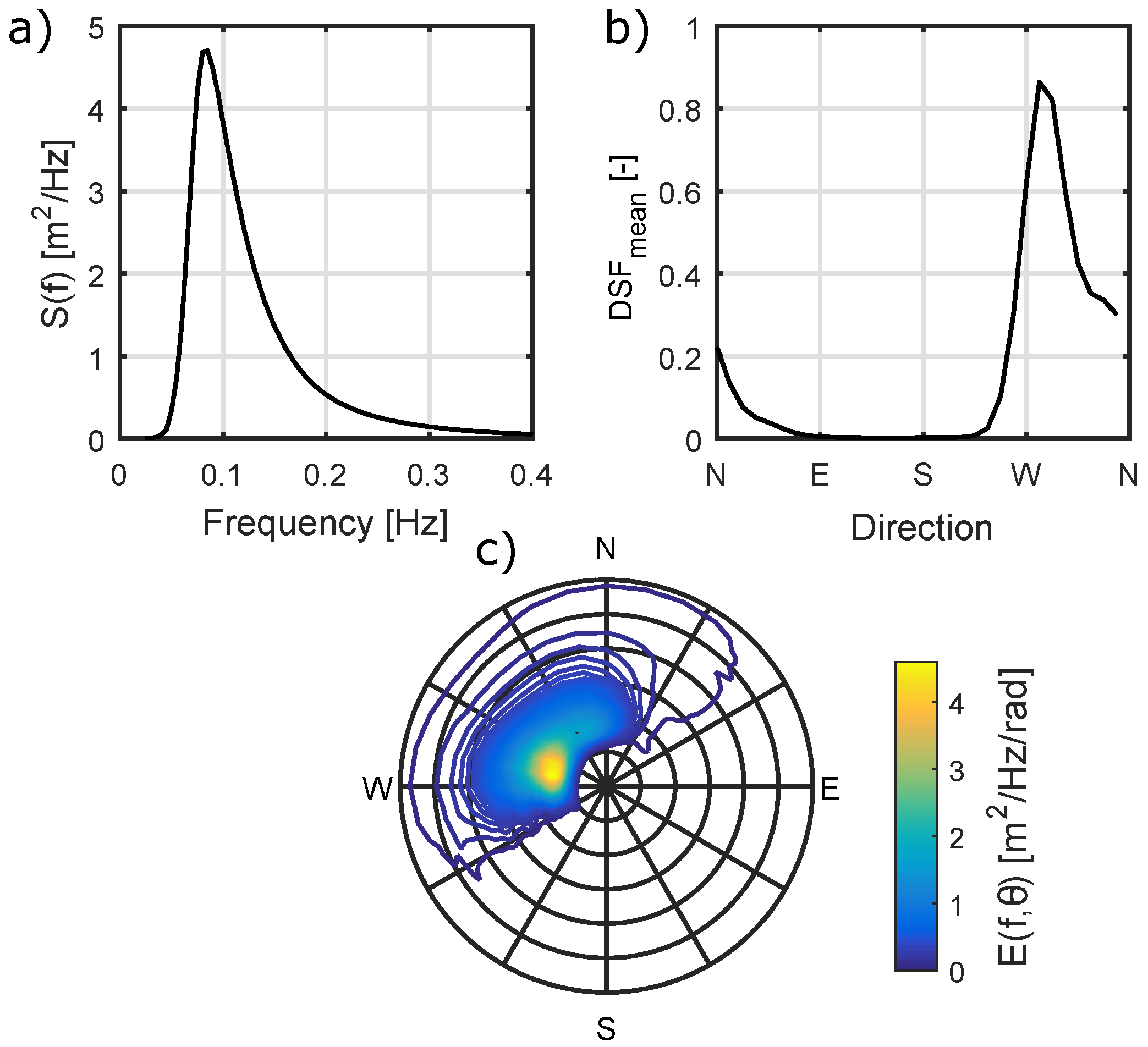
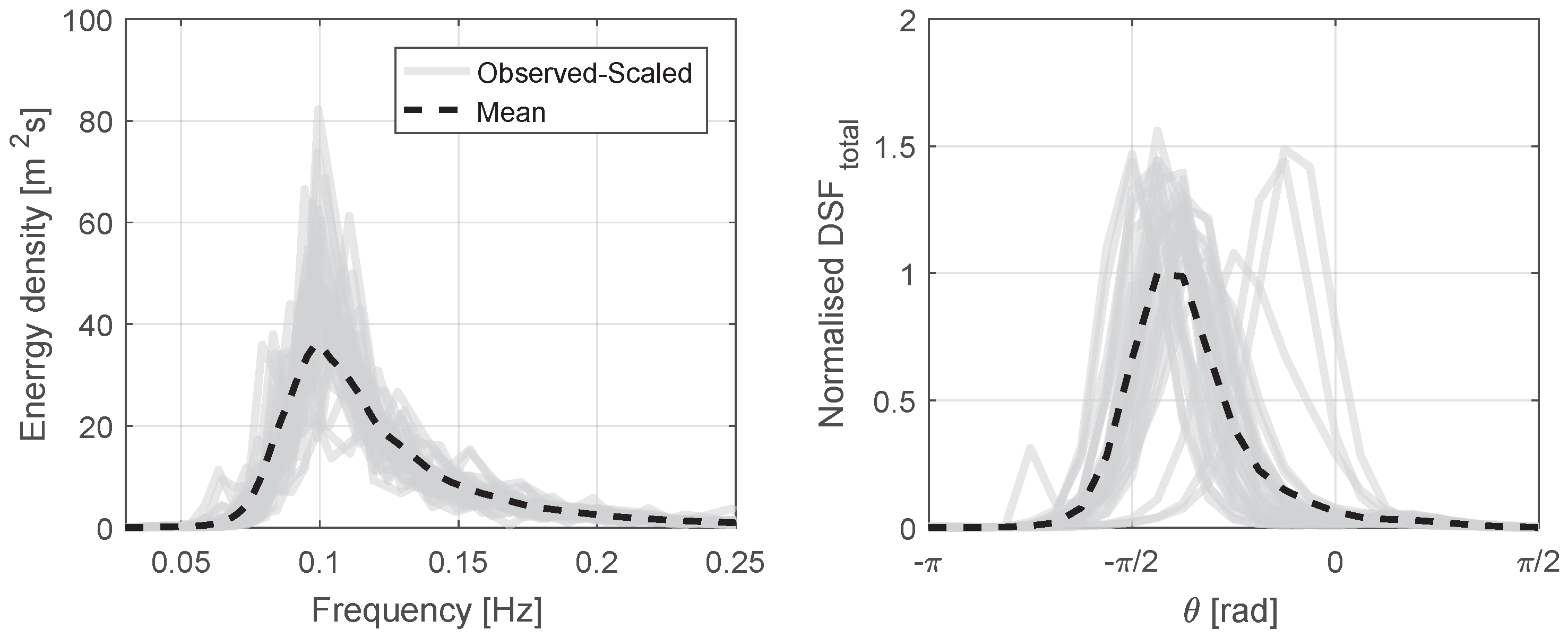
The frequency spectra, in combination with directional Fourier coefficients, have been used to estimate the directional distributions required in this analysis. This process is described in Section 2.2. The calculated mean frequency and directional spectra for the site, along with the mean weighted directional spreading function () is shown in Figure 1. Mean values of and are 2.05 m and 8.33 s respectively, with the most energetic recorded sea state having a of around 11.5 m, and of 15 s.
1.2. The FloWave Ocean Energy Research Facility
All experiments presented in this paper were carried out at the FloWave Ocean Energy Research Facility, Edinburgh, UK. The 2 m depth facility consists of a 25 m diameter wave basin encircled by 168 active-absorbing wavemakers, enabling waves to be generated from all angles. Sea states can therefore be created with arbitrary directional characteristics, and FloWave has been shown in to be able to effectively re-create complex multi-directional multi-modal spectra [17,18]. This allows the directional complexity of observed ocean conditions such as those defined in Section 2 to be effectively simulated.
2. Defining Extreme Directional Wave Conditions
This section deals with the extreme sea state definition, and aims to define a set of realistic directional spectra that are representative of extremes at the site. Section 2.1 shows how statistical parameters, and , can be appropriately associated with extreme events at specified return periods. In Section 2.2, these values are used to create realistic extreme sea states, which are based off observed directional spectra associated with storms at the site.
2.1. Defining Extreme Wave Height and Period
2.1.1. Significant Wave Height
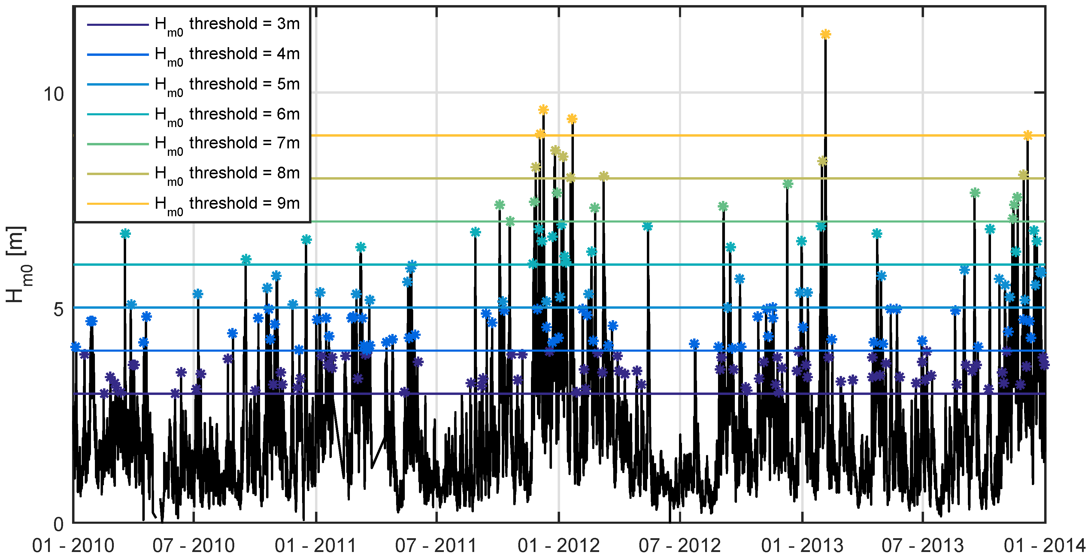
There are a variety of approaches for inferring the largest expected significant wave heights in a given time frame. For the initial peak identification a variety of methods can be employed, including the commonly used block maxima (BM) or peaks over threshold (POT) approaches [3], while an r-largest or average conditional exceedance rate (ACER) [19,20] methodology could equally be applied. It is recommended by Caires [3] that if the dataset is relatively small (a few years) then a POT approach should be taken. Additionally, if multiple storm events occur within relatively small time-frames, it is recommended in Teena et al. [4] to use this POT method to include all the extreme events in the analysis. As this is the case for the dataset available a POT approach will be used in this work. Figure 2 shows the points identified as POT-valid points for different thresholds. These points must be independent [3] and are ensured here by only considering the maximum points over the threshold, in the 24 h preceding and after the considered event.
BM derived data (such as annual maxima) require fitting with a generalised extreme value (GEV) distribution [3], which consists of well known different types [21]: Gumbel (type I), Fréchet (II) or reversed Weibull (type III) distributions. For threshold derived extreme data e.g., POT, Leadbetter [22] showed that a generalised pareto distribution (GPD) should be used, and as such, a POT-GPD analysis is deemed most appropriate for the dataset available. Similarly to GEV distributions there are different types of GPD depending on the value of the shape parameter : exponential (type I), Pareto (type II) and a form of beta-distribution (type III). The equations for the GPD is shown in Equations (2) and (3).
- where: = shape parameter, = scale parameter, = rate, u = threshold.
- Type I: = 0, Type II: > 0, Type III: < 0
Choosing the appropriate threshold for the POT analysis is a trade-off between bias and variance and must be small enough to ensure there are sufficient points to determine the GPD parameters, but also must be large enough so that the data is truly capturing extreme events, and as such converges to a GPD [23]. Based on the stability parameter defined in Caires [3] a threshold of 4 m was eventually chosen, considered large enough as to only consider extremes but include a sufficient number of points, while being associated with a ‘stable’ region, and with a high associated value. The final GPD distribution with the 4 m threshold is shown in Figure 3, with the observed data overlaid.
2.1.2. Energy Period
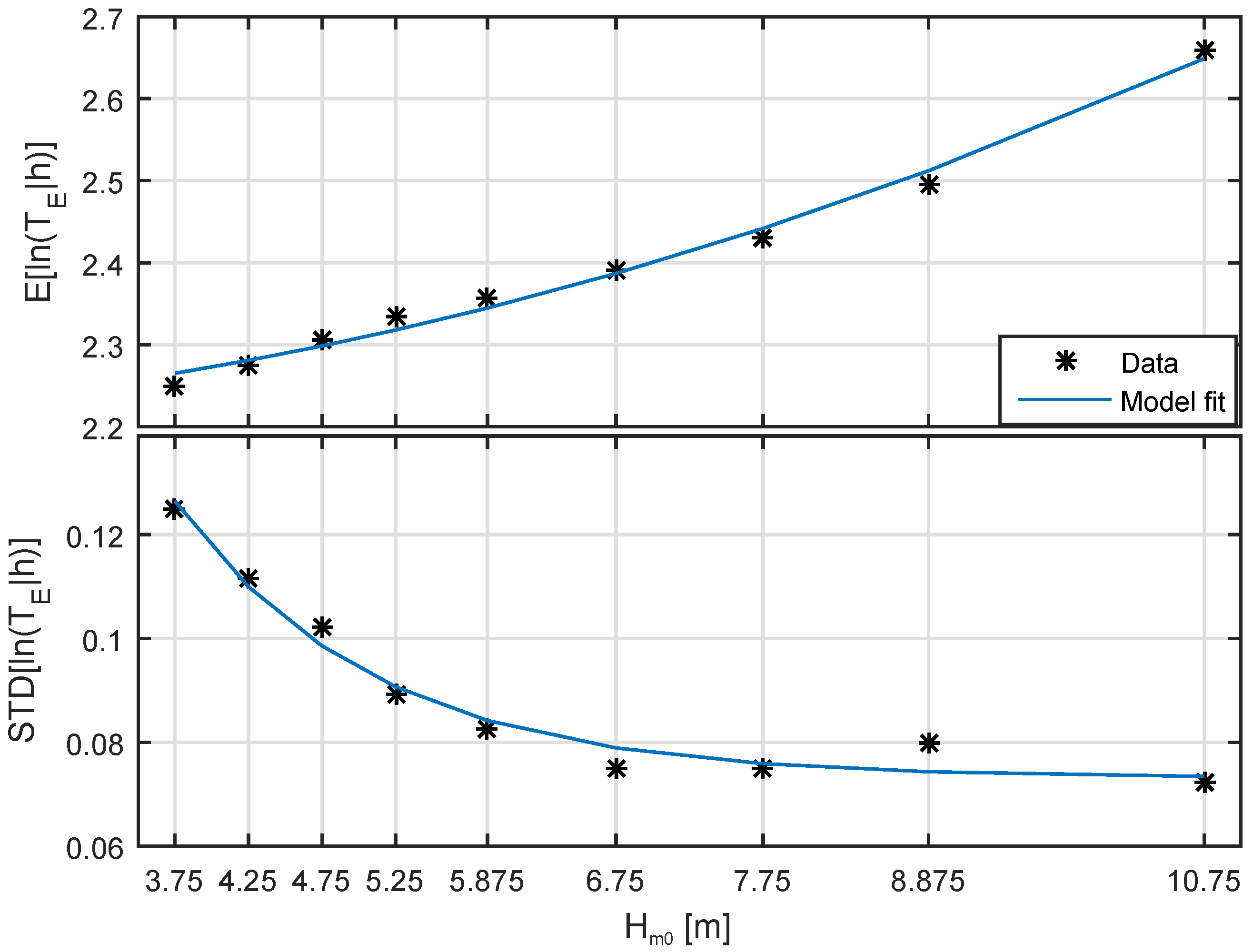
As mentioned in Section 1, to define extreme sea states effectively, appropriate wave period values are required. Log-normal distributions have been shown to effectively describe wave period distributions by Burrows and Salih [24], and therefore a parametrised conditional log-normal distribution has been fitted to values of energy period similar to Berg [7]. The parameters have only been fitted for values roughly corresponding to those above the POT threshold, under the assumption that there may be a different relationship between wave period and extreme wave heights than for the total dataset. Bin sizes for the parametrisation are also increased for large values of , to ensure there is enough data in each bin to get meaningful standard deviations. The resulting fit is shown in Figure 4, with the log-normal parametrisation described by Equations (4)–(7).
2.1.3. Combined Conditions
Using the I-FORM method the two probability distributions can now be used to create contours relating to specified return periods. This is achieved by defining to be the exceedance value of a standard normal variable relating to the specified return period, m. Two standard normal variables and are then defined along a circle so that their radius is equal to . The standard normal probability of exceedance corresponding to the values of and can then be used to find the equivalent values of and via the obtained distributions. As in Berg [7], this is described formally in Equations (8)–(10):
It is typical to inflate to account for approximating true stochastic response by its median value. From Winterstein et al. [6] and Berg [7] it is suggested to inflate using , with values of between 0.1 and 0.2. A value of 0.15 has therefore been chosen for this analysis, with the resulting contours for return periods of 1, 10, 50 and 100 years shown in Figure 5.
The choice of extreme – combinations for tank testing, or numerical modelling, is dependent on the nature of the resulting probability distributions and the sensitivities of the device being tested (e.g., [9])). As wave energy converters are typically very sensitive to wave frequency (see [16,25,26,27]) it seems advantageous to choose a range of values, enabling exploration of system response to extreme conditions at various dominant forcing frequencies. Device and mooring design will influence the decision significantly. Typically, however, conditions of large wave height but relatively low wave period values may typically correspond to resonant conditions of the device and thus maximum motions, or may be likely to cause steepness induced snatch loads in mooring lines (e.g., [28]). Maximum mooring extension may occur from large surge loads within high sea states, while the largest impact loads may occur when state power or significant wave height is at a maximum.
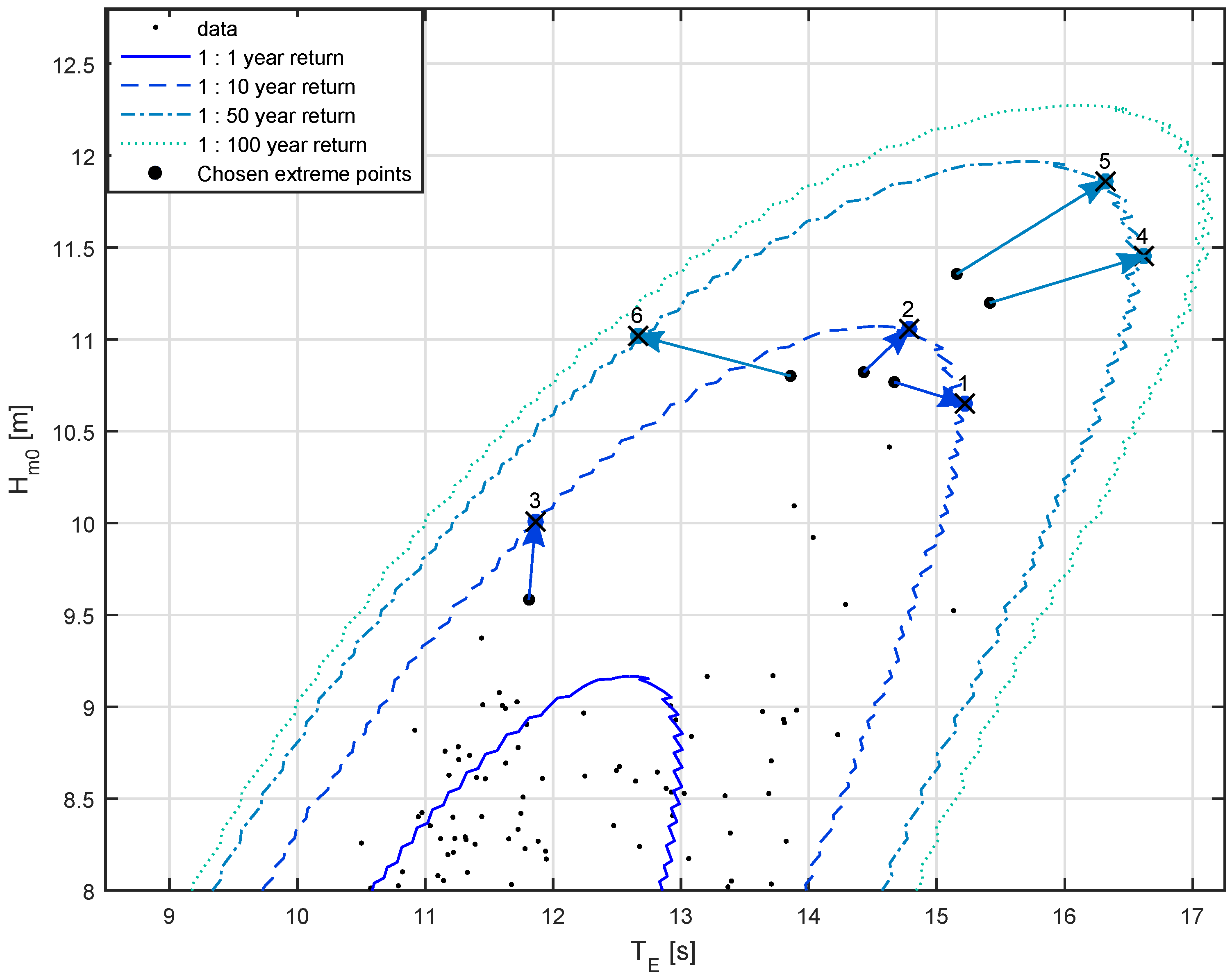
Various points have been chosen for 1:10 and 1:50 year extremes, to serve as an example cases for further analysis. The 1:10 year extremes are used as example extreme conditions which prototype devices may be subject to, with short deployments of a couple years. Extreme 1:50 year events will be more representative of full deployment lifetimes in the region of 20 years or more, as recommended by the International Electrotechnical Commission: IEC 61400-3 for offshore wind turbines [29], IEC 62600-2 for marine energy converters [30], and used in Ruiz [31] and Valamanesh et al. [32]. Points have been chosen corresponding to locations on each contour for maximum energy period, maximum power (normally maximum as well), and minimum above a threshold (10 m for 1:10, and 11 m for 1:50). The conditions specified, in combination with the extreme contours, define the combined extreme – values. These are shown in Table 1 and are highlighted in Figure 6. In this figure the closest unique observed data points are also highlighted, whose spectra are scaled to the desired – values in Section 2.2.2.
2.2. Defining Extreme Directional Spectra
2.2.1. Reconstructing Directional Spectra from Buoy Data
The buoy data available for the Billia Croo wave site does not explicitly include directional spectra, yet has directional Fourier coefficients which can be used as the basis for reconstruction. There are variety of methods available for the reconstruction of directional spectra, all of which have different assumptions and formulations, which results in DSFs which differ from each other significantly.
It is suggested in Nwogu et al. [33], Benoit [34], Benoit et al. [35], Kim et al. [36] that the maximum entropy principle (MEM2/MEP) is the most reliable for directional spreading estimates from single-point measuring systems like buoys. Despite this, the solution to the MEP is non-linear, computationally challenging and does not always converge. This led Hashimoto [37] to propose using Newton’s method of local linearisation to help the convergence and Kim et al. [36] to suggest approximate solutions to the problem. To avoid the convergence issues experienced with both the full MEP solution and the linearised approach, the aforementioned approximate solutions [36] have been used for this work, which have been found to give very similar directional spectra outputs to full solution equivalents.
2.2.2. Applying Scaling-Shifting Procedure to Observed Extreme Spectra
To define the extreme directional spectra, the ‘closest’ observed sea state to the defined extreme – points Table 1 are identified, using the M number defined in Equations (11) and (12). If a given observed sea state is the closest to multiple desired extreme points, distinct points are chosen that minimises total M number. Due to the relatively short dataset and low abundance of very high power sea states, there are conflicts for extreme conditions 1 and 2, along with 4 and 5. Forcing these sea states to be based on different observations allows the inclusion of differing conditions, highlighted in Figure 6.
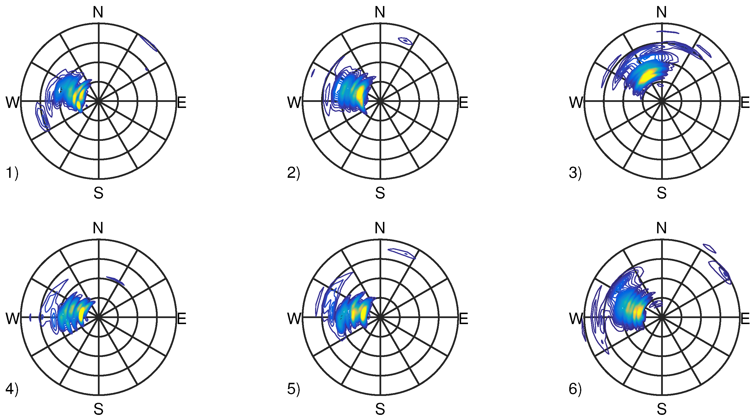
The selected sea states do not match the specified and values, and as such go through a scaling procedure. This required an amplification and a shifting in frequency. Noting that , Equation (13) can be used to get the correct by means of applying a single spectrum amplification factor. To obtain the correct , the whole spectrum is first interpolated to give a large number of frequency values. The spectrum is then shifted on the frequency axis until the desired is obtained. An iterative, rather than analytic, method was used here as is a function of i.e., to find the shift, the desired energy distribution would need to be known, which remains a function of the unknown frequency shift itself and the known spectral shape. The results from this scaling-shifting procedure for both the frequency and directional spectra are shown in Figure 7 and Figure 8 respectively. From Figure 8, it is evident that the resulting (observed) directional distributions are highly frequency dependent and would not have been obtained from a purely parametric approach to the sea state definition.
3. Simulating Extreme Directional Wave Conditions
This section covers the experimental aspect of this work: scaling, generating and validating the sea states. The defined sea states are scaled in Section 3.1, where difficulties are highlighted relating to a combination of depth and wavemaker constraints. Section 3.2 details the generation, measurement, and correction procedure and shows the final validated extreme spectra.
3.1. Scaling Sea States for Tank Tests
Froude scaling is used to scale sea states in order to obtain the correct ratio between inertial and gravitational forces, which are dominant for ocean waves. Ideally, all environmental conditions of a wave test are therefore Froude scaled, but there are constraints to consider, related to the sea state in question along with the characteristics and limitations of test facilities. Considering frequency dependent wave height limits of the FloWave facility, as well as absolute frequency limits of wave generation, it was found that the largest scale that the defined extreme sea states can be generated at effectively are 1:61. The desired scale factor is 1:26 (52 m site and 2 m tank), and as such, the sea state needs to be created at a non-depth-ratio.
In simple parametric cases, and values are typically used for scaling, which effectively results in Froude scaled frequency spectra, . However, if these are scaled and reproduced at any ratio other than the depth ratio, there are wavelength and power discrepancies to consider, differing from the desired Froude scaled values. For all but deepwater conditions, non-depth ratio scaling makes it is impossible to Froude scale all elements of a sea state [38]. Table 2 details how these errors can be calculated. In this table the subscript s refers to Froude scaled values, to full-scale values, and o to obtained values i.e., those that are not directly scaled and where errors arise. Alternative scaling approaches are also presented, which allow preservation of energy distributions across wavenumber, , and wave power across frequency, .
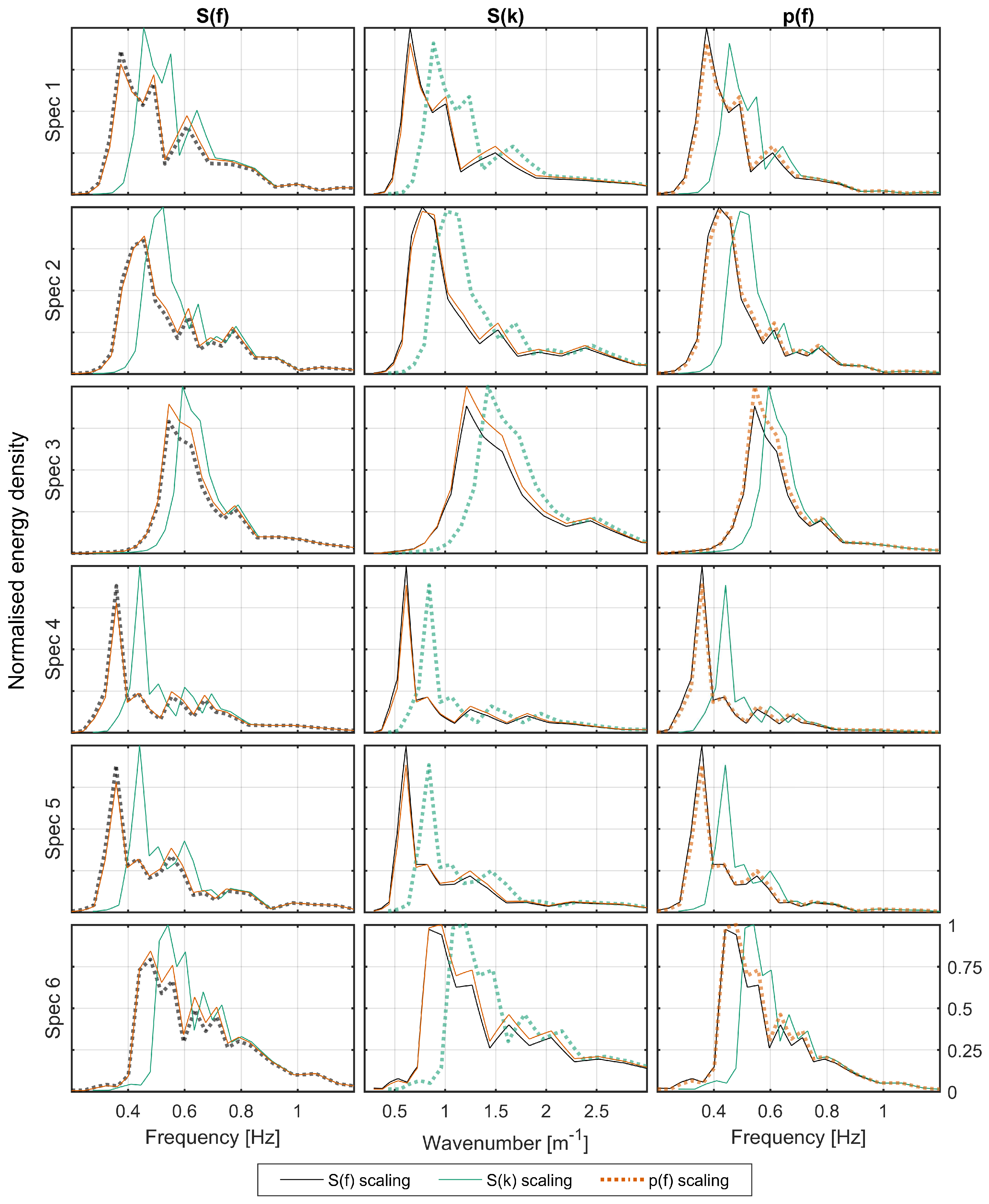
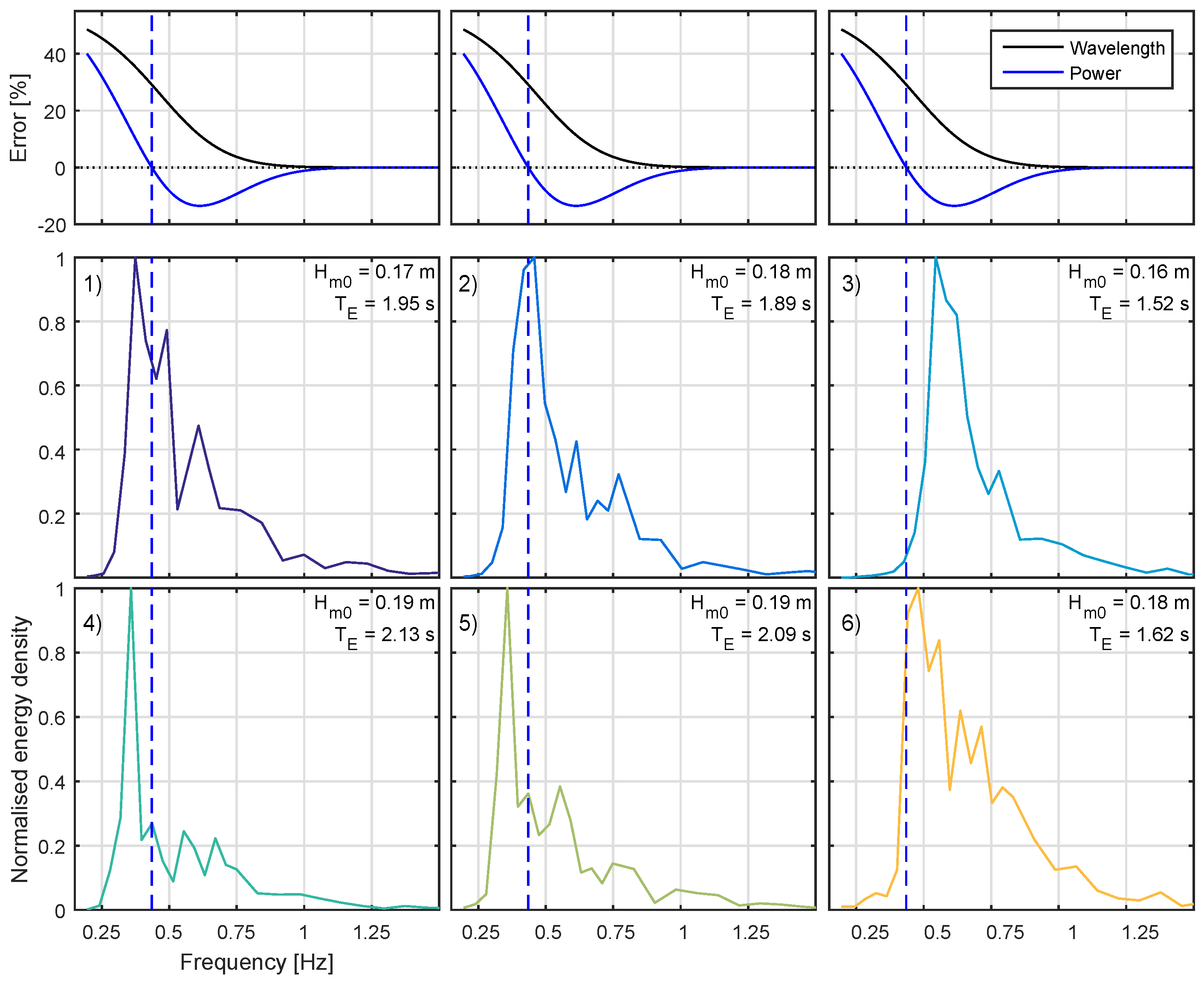
The 1:61 Froude scaled extreme frequency spectra are shown in Figure 9, with the power and wavelength errors incurred by non-depth-ratio scaling. It is interesting to note the changing sign of the frequency dependent wave power error at around 0.4 Hz: low frequency components have an over-representation of power while higher frequency components display lower power than desired. Above around 1.1 Hz (tank scale) wave frequencies that were in deep water at full scale remain to be in deep water at tank scale and as such power and wavelength are Froude scaled effectively. Importantly, total sea state power, , does not Froude scale in this case, with the total discrepancy dependent on the spectral shape. For this study, to demonstrate the ability to re-create the extreme sea states the scaled spectra have been used. The difference between the different scaling approaches are highlighted further in Appendix A: Figure A1, whereby the six extreme spectra are scaled using the three approaches described. This highlights the difference between the desired spectra at that scale and those obtained using the different scaling methodologies.
3.2. Generating, Measuring and Validating Extreme Directional Sea States
The Froude scaled directional spectra, , have been created in the FloWave basin, prior to measurement and correction based on the incident spectrum. To generate the directional sea states, the single-summation method [39] has been used, minimising phase-locking between frequency components and thus increasing the ergodicity of the wave field. Sea states have been created with a repeat time, T, of 2048 s and a run-time of 2100 s. This test length provides roughly a thousand waves, suggested in [40] to be the typical length of a storm, and should provide a good representation of individual extreme wave heights. A directional array of eight resistance type wave gauges (shown in [18]) has been deployed in the centre of the FloWave basin.
The Single-summation PTPD Approach with In-line Reflection (SPAIR) method [18] has been used to isolate the incident and reflected directional spectra. The method has been applied over the final 2048 s of the 2100 s measurement, corresponding to the defined sea state repeat time. This ensures that high frequency waves have had sufficient time to propagate to the measurement area, and that the assumption of stationarity is more valid. In addition, taking the measurement over exactly one repeat time ensures that every generation frequency component has undergone an even number of cycles and spectral leakage should be minimised. Due to slight under-generation, the incident wave spectrum is corrected using frequency dependent amplitude based correction factors as defined in Equation (14). This is repeated until mean spectral errors, (Equation (15)), are below 5%, which happens for all six sea states after a single iteration.
The final incident frequency spectra are shown in Figure 10, along with the desired spectrum and the calculated frequency dependent reflection coefficients. Corresponding weighted DSFs are shown in Figure 11, while the total directional spectra are displayed in Figure 12. It is evident that the measured sea states are very close to the desired and the directional and frequency distributions have been created to a high degree of accuracy. Discrepancies in frequency spectra are extremely low, as demonstrated by Figure 10, while the shape of the incident directional spreading match very closely with the desired distributions (Figure 11 and Figure 12). Reflection coefficients are generally low (below about 1 Hz), and discrepancies are well defined. This demonstrates that the complex defined energy distributions have been well produced, and that realistic directional extreme sea states are possible to simulate.
4. Discussion
This paper demonstrates a process of simulating realistic extreme directional sea states using wave buoy data and observed extremes: from site data to validation at tank scale. There is some interesting discussion to be had over the validity of the presented process, with particular issues evident when applied to the current dataset and re-created in the FloWave facility. This includes the – contour creation, the scaling-shifting procedure at full scale, and the Froude scaling trade-offs highlighted in Section 3.1. These issues are expanded upon below.
4.1. – Contour Creation
In Section 2, four years of buoy data was used to define extreme distributions of and combined –. This is not enough data to effectively capture inter-annual variability, and ideally a larger dataset would be used, particularly for gaining confidence in extrapolating 1:50 year events. This would reduce the large uncertainty in the return values (Figure 3). To check the obtained values were reasonable, comparison has been made to Lawrence et al. [41] where an extreme distribution is obtained for the site using a 20-year hindcast model. 1:10 and 1:100 year values were found to be around 10.7 m and 12 m respectively, which compares favourably to the 11 m and 12.2 m found in this analysis. This provides increased confidence in the presented analysis technique as these hindcast values should be relatively accurate.
I-FORM contours were created in order to obtain combined – values suitable for extreme sea state definition. In this process a parametrisation of the conditional probability of on is carried out, with the fit of log-normal parameters shown in Figure 4. Figure 5 shows the resulting contours, and it is evident that some observed values are outwith the 1:100 year contour. This is due to the requirement to parametrise the conditional distributions of , and again is somewhat a result of having a small dataset. A different (and likely more accurate for low values) parametrisation would have been found if more data was available.
It is worth re-visiting the fact that the and values these contours are derived from have been based on 30 min data samples. If these were calculated using longer time periods, such as the three hours sometimes used (and typically used in numerical models), then the observed extreme values would be slightly reduced. This would consequently provide smaller estimates of the expected extreme wave conditions. Assessing the current dataset, using three hour moving averages causes the maximum to reduce from 11.36 m to 10.77 m, and maximum down from 17.39 s to 16.79 s (for 3 hour blocks this becomes 10.34 m and 16.27 s respectively). This demonstrates the potential discrepancy caused by the sample length choice, whilst also highlighting one of the inherent difficulties in analysing ocean wave data. A compromise must be made so that the assumption of stationarity is valid, while simultaneously obtaining enough samples to have reasonably small uncertainty in spectral and statistical estimates. Whether 30 min or longer samples are more appropriate for extreme value analysis is therefore a matter of debate. For this work, however, the 30 min sample length was chosen because it is widely suggested (e.g., Euan et al. [42] and Alvarez-Esteban et al. [43]) to ensure that both the assumption of stationarity and ergodicity are reasonable.
4.2. Scaling-Shifting Procedure
4.2.1. Magnitude of Transformation
Observed spectra were used to define the test conditions. In order to ensure they matched the defined – values they were amplified () and shifted (). The resulting alteration to observed spectra are shown in Figure 7. This process is clearly only reasonable for small shifts in and . It is noted, however, that variation in observed spectral shapes over short time-frames (30 min) are many times larger than the ones proposed here, suggesting that the magnitude of the applied transformations may be reasonable, if not physically representative of wave energy transfer mechanisms. This change in spectral shapes for the 3 h prior to each identified extreme point is shown in Figure 13. From this figure, it is evident that there are quite significant changes in both and over relatively short time-frames. This aids somewhat in putting the proposed changes to the observed spectra into perspective.
This extreme value analysis aims to identify and create improbable conditions, yet care must be taken to ensure the test spectra are not impossible. Despite the example transformations being reasonable, it must be ensured that changes are not too large and do not breach any physical laws. In particular, if increasing significantly and/or reducing , then the new steepness must be calculated to ensure that the proposed spectrum is still physically maintainable and wave steepness limits are not breached. Equally, shifting a spectrum to have a much larger wave period may also represent an impossible energy distribution given the fetch length available. Therefore, in addition to checking steepness, it seems that a limit should be placed on the overall transformation.
From observation of the transformed spectra in Figure 7, it is suggested that the required scaling for the 1:10 year example events are very minor, well within typical spectral uncertainty, and hence represent a valid change. Relative to the large scale variations over short time frames, it also appears that scaling sea states for the 1:50 year events may also be reasonable. However, some of the large changes in the energy period required for some of these sea states, particularly Extreme 6, make this more questionable. Despite these concerns, the applied frequency shift seems to still create plausible conditions, due to the occurrence of many sea states with larger values, up to 25 s (0.04 Hz) in the dataset.
On the basis of these observations, and noting the associated M values from Equation (11), it seems reasonable to suggest that any M value of less than 0.05 would be a very minor required change and hence clearly acceptable. It is suggested, based on the magnitude of the changes relative to observed variations over half-hour periods, that M values of less than 0.1 are also potentially acceptable, as long as both general and site-specific physical laws are not broken.
4.2.2. Spectral Variability
The methodology applied in this paper gives emphasis on preserving the form of observed directional spectra. The idea behind this approach is that it ensures resulting spectral definitions of extreme events are both possible and characteristic of those in the defined – region. For certain values of and the possible and likely range of spectral shapes, both in frequency and direction, may vary significantly i.e. there may be a wide range of underlying ocean conditions that can provide the same statistics. For other values, particularly those which represent highly energetic sea states, the range of possible conditions will be smaller. Inherent limits on steepness and the necessity to have large fetch lengths will impose limits on plausible predominant propagation directions, directional spreading and peak frequencies of the wave system. It is both important, and interesting, to explore the likely spectral variation, as to put into context the work presented.
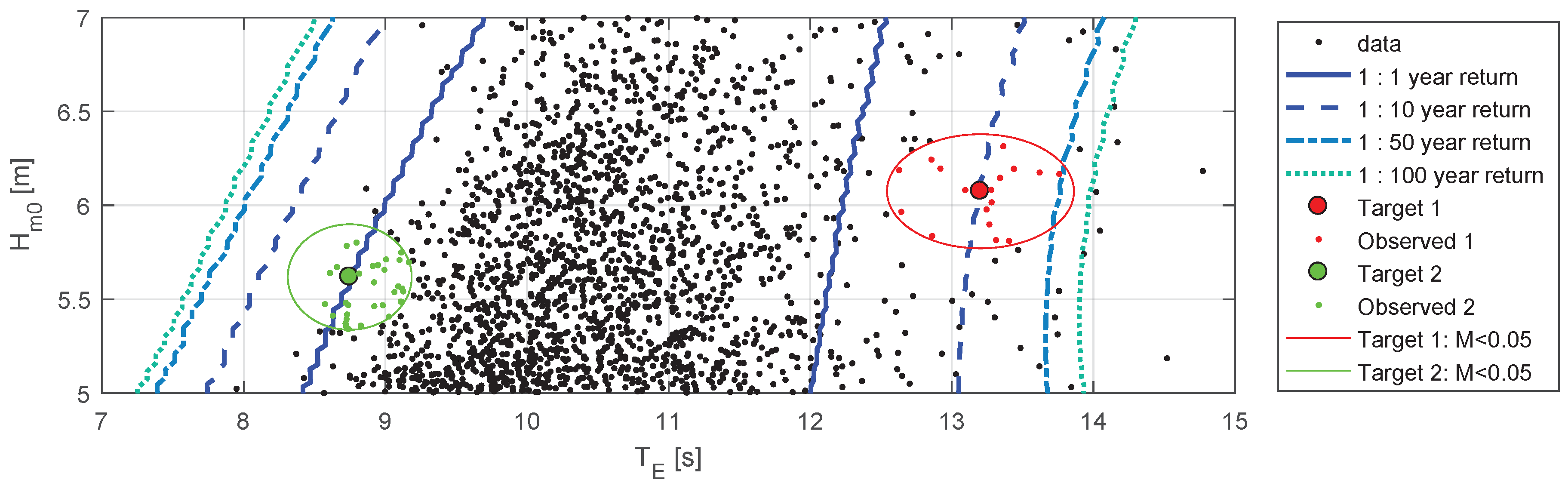
The expected variation for very extreme events at the site is difficult to explore in this instance as the dataset is relatively small and observations of highly extreme conditions are limited. To explore the expected spectral variation, two examples are presented where there a number of observation points, one for low conditions and one for high . These examples allow for identification of the expected spectral variability for different wave conditions, but also helps put into perspective the emphasis placed on individual spectral forms throughout this work.
All points with to the specified conditions are scaled to the desired values and compared. The two points identified are shown in Figure 14, along with the observed points within the region. These desired points were chosen as the differing values will relate to different underlying physical wave conditions (and there are a reasonable number of observation points to analyse).
The spectra and frequency-averaged DSF’s for the high and low examples are shown in Figure 15 and Figure 16 respectively. It is evident from these figures that, for the high case, observed frequency spectra are reasonably similar, with low peak frequencies and narrow spectral bandwidths. Also suggested from the selected data is that large period storms are likely to originate from a particular direction (north-west). The necessity to have a large fetch length also means that there is essentially a spatial filter applied which limits, and practically standardises, the observed directional spreading. For the low example this is not the case. Frequency spectra are similar to each other, with increased peak frequencies and spectral bandwidths, yet much greater variation is observed in the directional spreading than observed in the high case. The lower energy periods mean that these sea states do not have the same fetch requirements, and comprise of more locally driven, and very steep, ‘wind-driven’ seas which can originate from a larger variety of directions.
The results of this analysis demonstrate that, although the method presented ensures likely and realistic directional wave conditions to be used, it does not guarantee that all of the possible ‘types’ of spectral conditions are identified. This is potentially an issue that could be resolved with a larger dataset. Increased extreme observations would allow for the identification of different spectral types related to specified – definitions. With a more extensive dataset, or by choosing less extreme – combinations which are more abundant, the different associated spectral types can incorporated into a tank testing program. This approach, when achievable, will improve the presented methodology and further aid de-risking WEC’s in realistic extreme wave conditions.
4.3. Froude Scaling Issues
As mentioned in Section 3.1, it was not possible to Froude scale all elements of the extreme sea states in FloWave. This is because Froude scaling is never fully achievable for intermediate water conditions when depth-ratio scales are not attainable. Froude scaled & were used to demonstrate the process of re-creating, correcting and validating sea states in Section 3.1, however, this was essentially an arbitrary choice. If the device being tested is very sensitive to wavelength or wave steepness (e.g., attenuator type WEC) then it is probably more appropriate to scale wavenumber spectra, , ensuring the correct distribution of energy across the different wavelengths. A point absorber WEC may be mostly responsive to different frequencies of waves and as such scaling is favourable, while scaling may provide the best representation for power production tests rather than testing in extreme conditions.
The outcomes of extreme tank tests feed back into design of offshore structures and renewable energy devices, and can affect the design and total cost significantly. It is, therefore, important to maximise both the relevance and accuracy of tests and results so that design decisions are well informed. Where possible it is recommended to use facilities where depth-ratio scaling can be achieved. This, however, is often problematic for the creation of extreme sea states due to wavemaker limits and limited ranges of tank depths. In such scenarios, as presented here, where depth-ratio scaling is not achievable, it is suggested that both and scaled sea states are used in testing and the results compared. The worst case (e.g., maximum load case) should then be considered for design.
5. Conclusions
Extreme wave conditions are simulated in physical model testing to assess survivability of offshore structures and devices, and can have a large influence over design and eventual cost. Tank tests that simulate extremes should therefore ensure the conditions generated are representative of the deployment site, and are accurately re-produced. In this paper we present a method of achieving this, using site data, inverse-first order reliability method (I-FORM) contours, and observed extreme events to define realistic directional sea states for the Billia Croo wave site. Six differing extreme conditions are chosen relating to 1:10 and 1:50 year events, and are simulated at scale in the FloWave basin. The whole process from site data to tank scale validation is presented. Careful consideration must be given at each of the detailed stages, allowing scale reproduction of realistic directional extreme sea states to a high degree of accuracy. The inclusion of such conditions in tank testing programmes allows for increased, and more relevant, learning to occur prior to full-scale development and deployment.
Acknowledgments
The authors would like to thank the Energy Technologies Institute and RCUK Energy programme for funding this research as part of the IDCORE programme (EP/J500847/1), the UK EPSRC for funding the FloWave facility (EP/I02932X/1), and the European Marine Energy Centre for providing buoy data for the sea state replication work.
Author Contributions
Samuel Draycott developed the methodology and carried out the analysis, tank tests and write-up. Thomas Davey conceived of the project this work is part of, helped supervise and reviewed the paper. David M. Ingram also helped supervise, providing guidance throughout the project.
Conflicts of Interest
The authors declare no conflict of interest.
Appendix A. Frequency, Wavenumber and Power Spectrum Scaled Spectra
Figure A1.
Resulting extreme spectra scaled in different ways. Shown is the resulting , and spectra when the , or spectrum is Froude scaled. The desired Froude scaled value is shown as a dashed line, and colours represent the different scaling types.
Figure A1.
Resulting extreme spectra scaled in different ways. Shown is the resulting , and spectra when the , or spectrum is Froude scaled. The desired Froude scaled value is shown as a dashed line, and colours represent the different scaling types.
References
- Goda, Y. Random Seas and Design of Maritime Structures; World Scientific: Singapore, 2010. [Google Scholar]
- Coles, S.G. An Introduction to Statistical Modeling of Extreme Values; Springer-Verlag: London, UK, 2001; p. 221. [Google Scholar]
- Caires, S. Extreme Value Analysis: Wave Data; Technical Report, No. 57; Joint Technical Commission for Oceanography and Marine Meteorology (JCOMM): Geneva, Switzerland, 2011. [Google Scholar]
- Teena, N.V.; Sanil Kumar, V.; Sudheesh, K.; Sajeev, R. Statistical analysis on extreme wave height. Nat. Hazards 2012, 64, 223–236. [Google Scholar] [CrossRef]
- Haver, S.; Nyhus, K. A wave climate description for long term response calculations. In Proceedings of the Fifth International Symposium on Offshore Mechanics and Arctic Engineering, Tokyo, Japan, 13–18 April 1986. [Google Scholar]
- Winterstein, S.R.; Ude, T.C.; Cornell, C.A.; Bjerager, P.; Haver, S. Environmental Parameters for Extreme Response: Inverse Form with Omission Factors. In Proceedings of the ICOSSAR ’93, the 6th International Conference on Structural Safety and Reliability, Innsbruck, Austria, 9–13 August 1993. [Google Scholar]
- Berg, J.C. Extreme Ocean Wave Conditions for Northern California Wave Energy Conversion Device; Sandia National Laboratories: Albuquerque, NM, USA; Livermore, CA, USA, 2011.
- Davey, T.; Venugopal, V.; Girard, F.; Smith, H.; Smith, G.; Lawrence, J.; Caveleri, L.; Bertotti, L.; Prevosto, M.; Holmes, B. D2.7 Protocols for Wave and Tidal Resource Assessment; Technical Report, No. 213380; European Commission: Brussels, Belgium, 2010. [Google Scholar]
- Doherty, K.; Folley, M. Extreme Value Analysis of Wave Energy Converters. In Proceedings of the 21st International Offshore and Polar Engineering (ISOPE) Conference, Maui, HI, USA, 19–24 June 2011; Volume 8, pp. 557–564. [Google Scholar]
- Ochi, M.K.; Hubble, E.N. Six-Parameter Wave Spectra. In Proceedings of the 15th International Conference on Coastal Engineering, Honolulu, HI, USA, 11–17 July 1976; Volume 1, pp. 301–328. [Google Scholar]
- Mansour, A.E.; Ertekin, R.C. Report of technical committee I.1 environment. In Proceedings of the 15th International Ship and Offshore Structures Congress, 1st ed.; Elsevier Science: Amsterdam, The Netherlands, 2003; Volume 1. [Google Scholar]
- Saulnier, J.B.; Maisondieu, C.; Ashton, I.; Smith, G.H. Refined sea state analysis from an array of four identical directional buoys deployed off the Northern Cornish coast (UK). Appl. Ocean Res. 2012, 37, 1–21. [Google Scholar] [CrossRef]
- Saulnier, J.B.; Clément, A.; Falcão, A.F.D.O.; Pontes, T.; Prevosto, M.; Ricci, P. Wave groupiness and spectral bandwidth as relevant parameters for the performance assessment of wave energy converters. Ocean Eng. 2011, 38, 130–147. [Google Scholar] [CrossRef]
- Gilloteaux, J.C.; Ringwood, J. Influences of wave directionality on a generic point absorber. In Proceedings of the 8th European Wave and Tidal Energy Conference, Uppsala, Sweden, 7–10 September 2009; pp. 979–988. [Google Scholar]
- Zhang, S.; Zhang, J. A new approach to estimate directional spreading parameters of a cosine-2s model. J. Atmos. Ocean.Technol. 2006, 23, 287–301. [Google Scholar] [CrossRef]
- Holmes, B. Tank Testing of Wave Energy Conversion Systems; The European Marine Energy Centre Ltd (EMEC): Orkney, UK, 2009. [Google Scholar]
- Draycott, S.; Davey, T.; Ingram, D.M.; Lawrence, J.; Day, A.; Johanning, L. Applying Site-Specific Resource Assessment: Emulation of Representative EMEC seas in the FloWave Facility. In Proceedings of the 25th (2015) International Ocean and Polar Engineering Conference, Kona, HI, USA, 21–26 June 2015; pp. 815–821. [Google Scholar]
- Draycott, S.; Davey, T.; Ingram, D.M.; Day, A.; Johanning, L. The SPAIR method: Isolating incident and reflected directional wave spectra in multidirectional wave basins. Coast. Eng. 2016, 114, 265–283. [Google Scholar] [CrossRef] [Green Version]
- Naess, A.; Karpa, O. Statistics of bivariate extreme wind speeds by the ACER method. J. Wind Eng. Ind. Aerodyn. 2015, 139, 82–88. [Google Scholar] [CrossRef]
- Troldborg, N.; Sørensen, J. A simple atmospheric boundary layer model applied to large eddy simulations of wind turbine wakes. Wind Energy 2014, 17, 657–669. [Google Scholar] [CrossRef]
- Markose, S.; Alentorn, A. Option Pricing and the Implied Tail Index with the Generalized Extreme Value (GEV) Distribution 1. J. Deriv. 2011, 1–29. [Google Scholar] [CrossRef]
- Leadbetter, M.R. Extremes and local dependence in stationary sequences. Zeitschrift fur Wahrscheinlichkeitstheorie und Verwandte Gebiete 1983, 65, 291–306. [Google Scholar] [CrossRef]
- Abild, J.; Andersen, E.Y.; Rosbjerg, D. The climate of extreme winds at the great belt, Denmark. J. Wind Eng. Ind. Aerodyn. 1992, 41, 521–532. [Google Scholar] [CrossRef]
- Burrows, R.; Salih, B.A. Statistical Modelling of Long-Term Wave Climates. In Proceedings of the 20th International Conference on Coastal Engineering, Taipei, Taiwan, 9–14 November 1986; pp. 42–56. [Google Scholar]
- Goggins, J.; Finnegan, W. Shape optimisation of floating wave energy converters for a specified wave energy spectrum. Renew. Energy 2014, 71, 208–220. [Google Scholar] [CrossRef]
- Sheng, W.; Lewis, A. Assessment of Wave Energy Extraction From Seas: Numerical Validation. J. Energy Resour. Technol. 2012, 134, 041701. [Google Scholar] [CrossRef]
- Palm, J.; Eskilsson, C.; Paredes, G.M.; Bergdahl, L. Coupled mooring analysis for floating wave energy converters using CFD: Formulation and validation. Int. J. Mar. Energy 2016, 16, 83–99. [Google Scholar] [CrossRef]
- Hann, M.; Greaves, D.; Raby, A. Snatch loading of a single taut moored floating wave energy converter due to focussed wave groups. Ocean Eng. 2015, 96, 258–271. [Google Scholar] [CrossRef]
- International Electrotechnical Commission. IEC 61400-3: Wind Turbines—Part 1: Design Requirements; International Electrotechnical Commission: Geneva, Switzerland, 2005. [Google Scholar]
- International Electrotechnical Commission. PD IEC/TS 62600-200: 2016 Marine Energy—Wave, Tidal and Other Water Current Converters Energy Converters; International Electrotechnical Commission: Geneva, Switzerland, 2016. [Google Scholar]
- Ruiz, M.T. Dynamics and Hydrodynamics for Floating Wave Energy Converters; Technical Report; Instituto Superior Técnico: Lisbon, Portugal, 2010. [Google Scholar]
- Valamanesh, V.; Myers, A.T.; Arwade, S.R. Multivariate analysis of extreme metocean conditions for offshore wind turbines. Struct. Saf. 2015, 55, 60–69. [Google Scholar] [CrossRef]
- Nwogu, O.; Mansard, E.; Miles, M.; Isaacson, M. Estimation of directional wave spectra by the maximum entropy method. In Proceedings of the IAHR Seminar on Wave Analysis and Generation in Laboratory Basins, 22nd IAHR Congress, Lausanne, Switzerland, 31 August–4 September 1987; pp. 363–376. [Google Scholar]
- Benoit, M. Practical comparative performance survey of methods used for estimating directional wave spectra from heave-pitch-roll data. In Proceedings of the 23rd International Conference on Coastal Engineering, Venice, Italy, 4–9 October 1992. [Google Scholar]
- Benoit, M.; Frigaard, P.; Schaffer, H.A. Analyzing multidirectional wave spectra: A tentative classification of available methods. In Proceedings of the 1997 IAHR Conference, San Francisco, CA, USA, 1–12 November 1997; pp. 131–158. [Google Scholar]
- Kim, T.; Lin, L.H.; Wang, H. Application of Maximum Entropy Method to the Real Sea Data. Coast. Eng. 1994, 24, 340–355. [Google Scholar]
- Hashimoto, N. Analysis of the directional wave spectra from field data. Adv. Coast. Ocean Eng. 1997, 3, 103–144. [Google Scholar]
- Noble, D.R.; Draycott, S.; Davey, T.A.; Bruce, T. Design diagrams for wavelength discrepancy in tank testing with inconsistently scaled intermediate water depth. Int. J. Mar. Energy 2017, 18, 109–113. [Google Scholar] [CrossRef]
- Miles, M.D.; Funke, E.R. A Comparison of Methods for Synthesis of Directional Seas. J. Offshore Mech. Arct. Eng. 1989, 111, 43–48. [Google Scholar]
- Grice, J.R.; Taylor, P.H.; Taylor, R.E. Second-order statistics and ‘designer’ waves for violent free-surface motion around multi-column structures. Philos. Trans. R. Soc. Lond. A Math. Phys. Eng. Sci. 2015, 373, 20140113. [Google Scholar] [CrossRef] [PubMed]
- Lawrence, J.; Kofoed-Hansen, H.; Chevalier, C. High-resolution metocean modelling at EMEC’s (UK) marine energy test sites. In Proceedings of the 8th European Wave and Tidal Energy Conference, Uppsala, Sweden, 7–10 September 2009; pp. 1–13. [Google Scholar]
- Euan, C.; Ortega, J.; Alvarez-esteban, P.C. Detecting Stationary intervals for random waves using time series. In Proceedings of the ASME 2014 33rd International Conference on Ocean, Offshore and Arctic Engineering OMAE 2014, San Francisco, CA, USA, 8–13 June 2014. [Google Scholar]
- Alvarez-Esteban, P.C.; Euán, C.; Ortega, J. Time Series Clustering using the Total Variation Distance with Applications in Oceanography. Environmetrics 2015, 27, 355–369. [Google Scholar] [CrossRef]
Figure 1.
Mean frequency spectrum (a), (b) and directional spectrum (c) for EMEC’s Billia Croo wave test site.
Figure 1.
Mean frequency spectrum (a), (b) and directional spectrum (c) for EMEC’s Billia Croo wave test site.

Figure 2.
Demonstration of correct Peaks Over Threshold (POT) identification. To be considered a peak, each point over the threshold must be the maximum in the 24 h preceding and after the point of interest. Four years of data is shown, from 1 January 2010 to 31 December 2013.
Figure 2.
Demonstration of correct Peaks Over Threshold (POT) identification. To be considered a peak, each point over the threshold must be the maximum in the 24 h preceding and after the point of interest. Four years of data is shown, from 1 January 2010 to 31 December 2013.

Figure 3.
Resulting final GPD distribution for extreme significant wave heights using the chosen POT threshold of 4 m. 95% confidence intervals are also shown.
Figure 3.
Resulting final GPD distribution for extreme significant wave heights using the chosen POT threshold of 4 m. 95% confidence intervals are also shown.
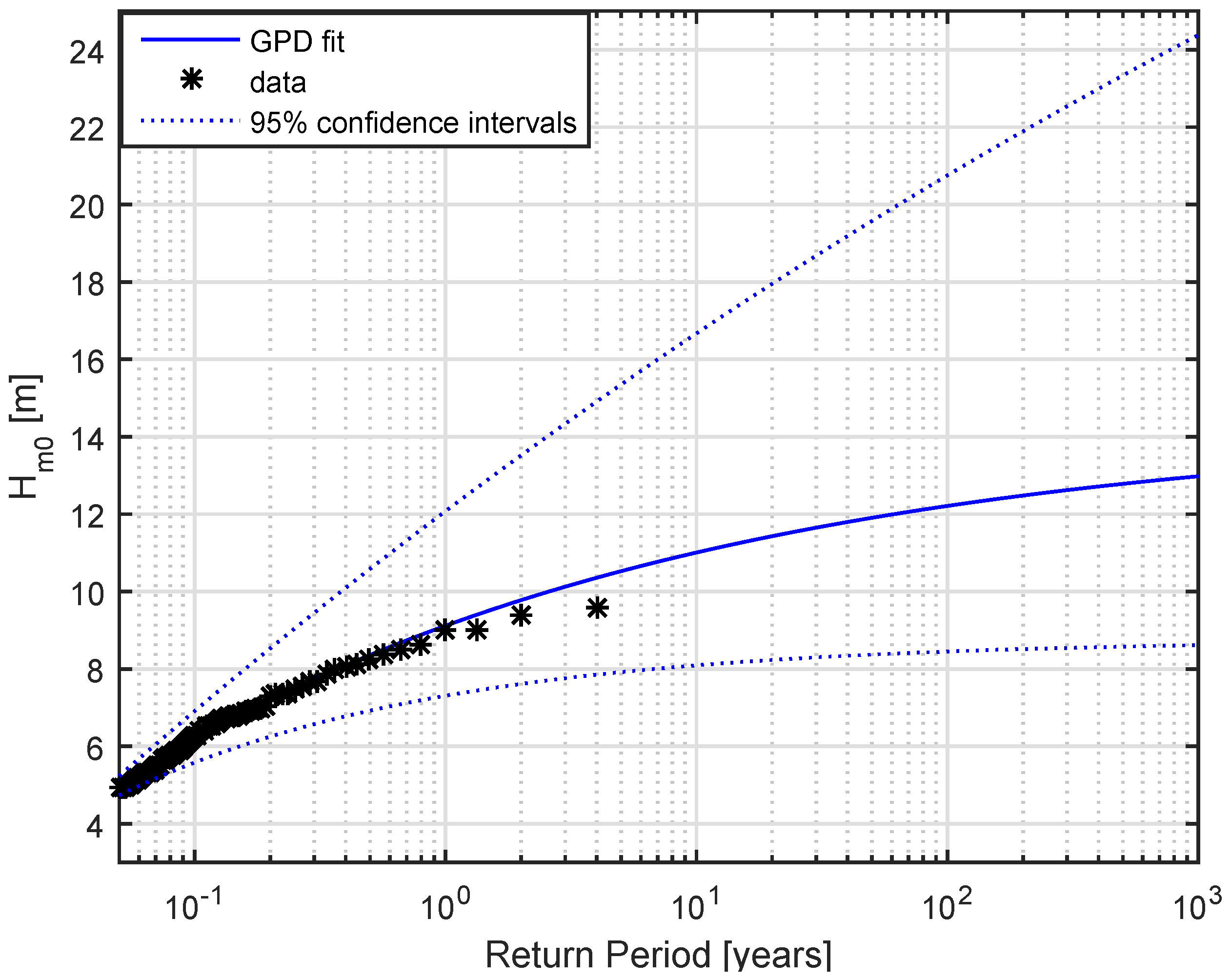
Figure 4.
Fit of log-normal parameters for conditional probability distributions of (conditional on ).
Figure 4.
Fit of log-normal parameters for conditional probability distributions of (conditional on ).

Figure 5.
I-FORM contours based on bivariate probability density function. 1:1, 1:10, 1:50 and 1:100 – contours created, shown with contours of wave power (deep water equivalent). Four years of buoy data is shown from the European Marine Energy Centre, and has been used to define the shown.
Figure 5.
I-FORM contours based on bivariate probability density function. 1:1, 1:10, 1:50 and 1:100 – contours created, shown with contours of wave power (deep water equivalent). Four years of buoy data is shown from the European Marine Energy Centre, and has been used to define the shown.
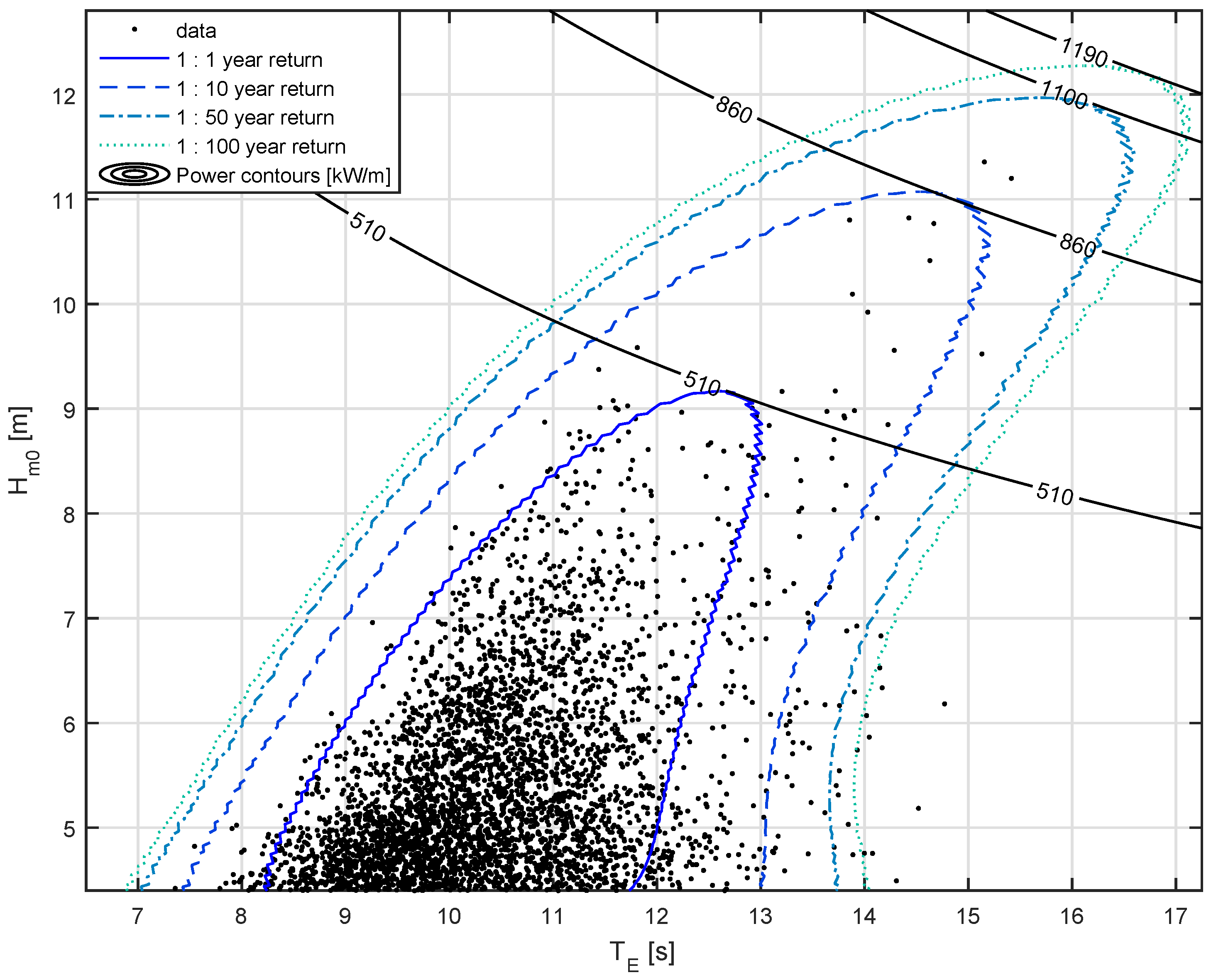
Figure 6.
Bivariate extreme contours with data points identified that have been chosen for scaling (large black circles). Crosses on the contours show the desired – values (Table 1), and arrows indicate which observed sea state is chosen to match each specified extreme condition.
Figure 6.
Bivariate extreme contours with data points identified that have been chosen for scaling (large black circles). Crosses on the contours show the desired – values (Table 1), and arrows indicate which observed sea state is chosen to match each specified extreme condition.

Figure 7.
Frequency spectra for sea states identified in Figure 6, scaled to desired extreme conditions (Table 1). M value overlaid corresponding to Equation (11).
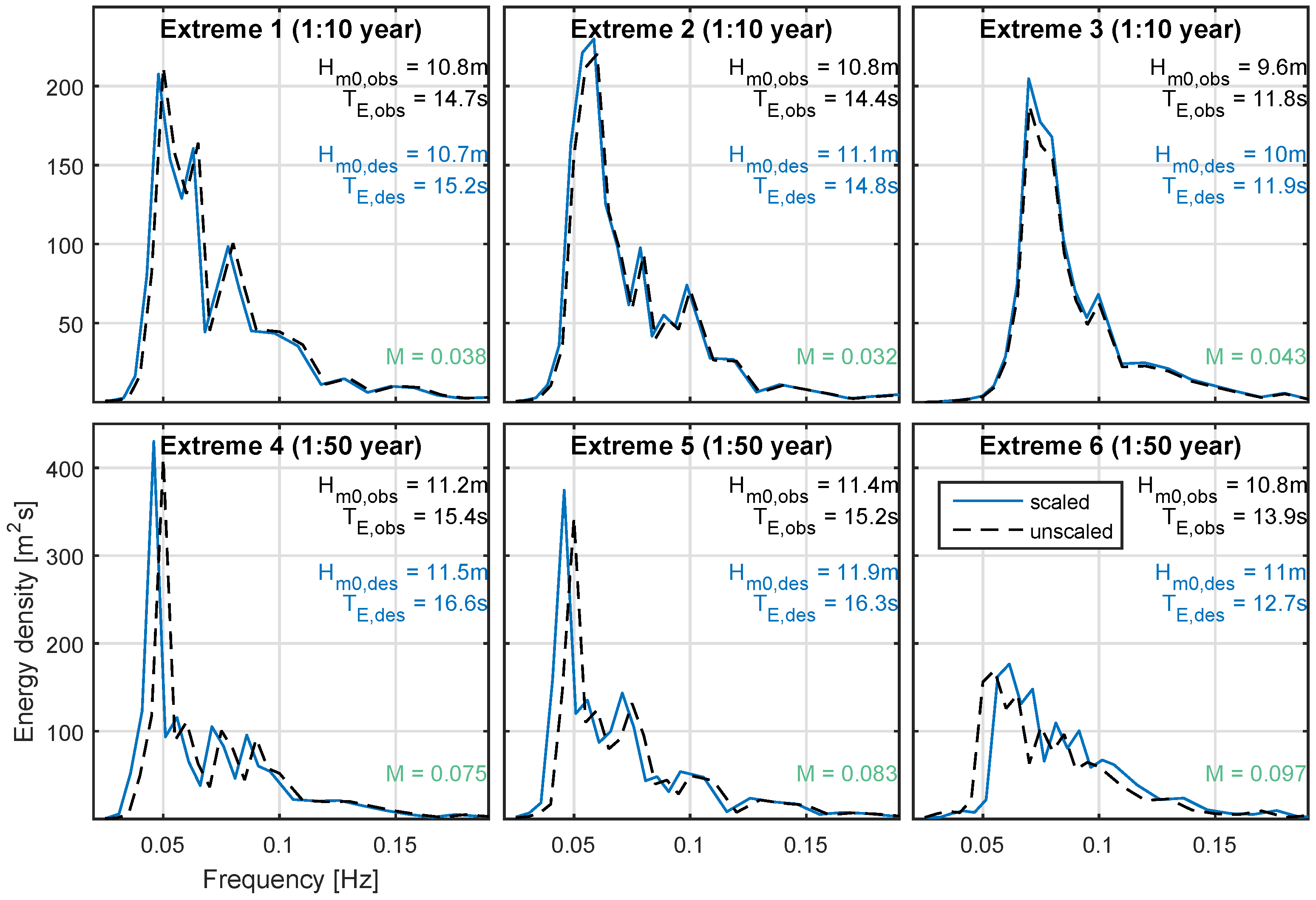
Figure 8.
Directional spectra for identified extreme sea states, scaled to desired extreme conditions. 1) to 6) correspond to sea states 1 to 6 defined in Table 1.
Figure 8.
Directional spectra for identified extreme sea states, scaled to desired extreme conditions. 1) to 6) correspond to sea states 1 to 6 defined in Table 1.

Figure 9.
Extreme sea frequency spectra Froude scaled at 1:61. Resulting relative frequency dependent wavelength and power errors at this scale shown above. Dashed blue line indicated the frequency where power errors change sign (at this scale and depth ratio). 1) to 6) correspond to sea states 1 to 6 defined in Table 1.

Figure 10.
SPAIR incident frequency spectrum outputs for the extreme sea states, compared with desired. Shown with calculated frequency dependent reflection coefficients. 1) to 6) correspond to sea states 1 to 6 defined in Table 1.
Figure 10.
SPAIR incident frequency spectrum outputs for the extreme sea states, compared with desired. Shown with calculated frequency dependent reflection coefficients. 1) to 6) correspond to sea states 1 to 6 defined in Table 1.
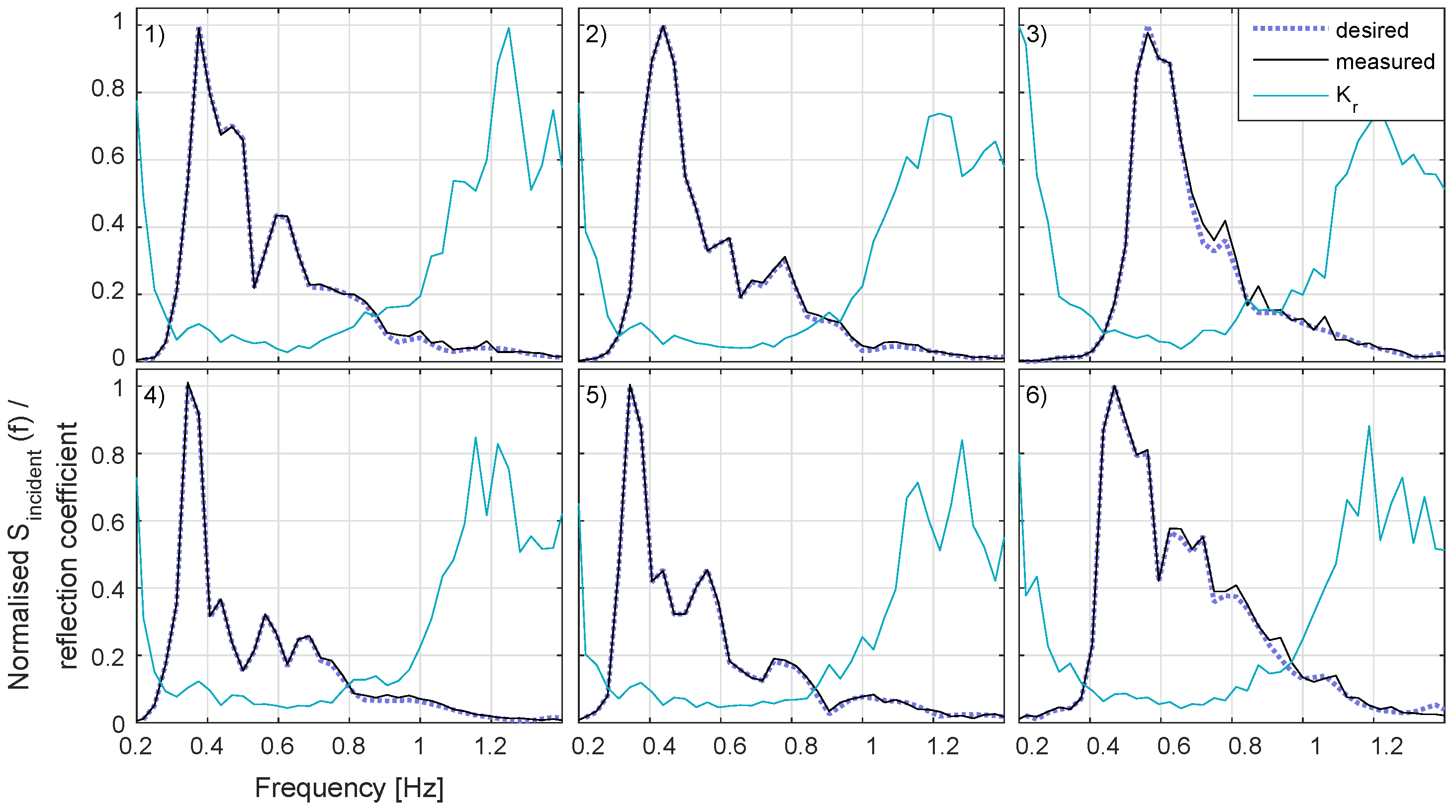
Figure 11.
SPAIR method weighted DSF outputs for the extreme sea states, compared with desired. 1) to 6) correspond to sea states 1 to 6 defined in Table 1.
Figure 11.
SPAIR method weighted DSF outputs for the extreme sea states, compared with desired. 1) to 6) correspond to sea states 1 to 6 defined in Table 1.
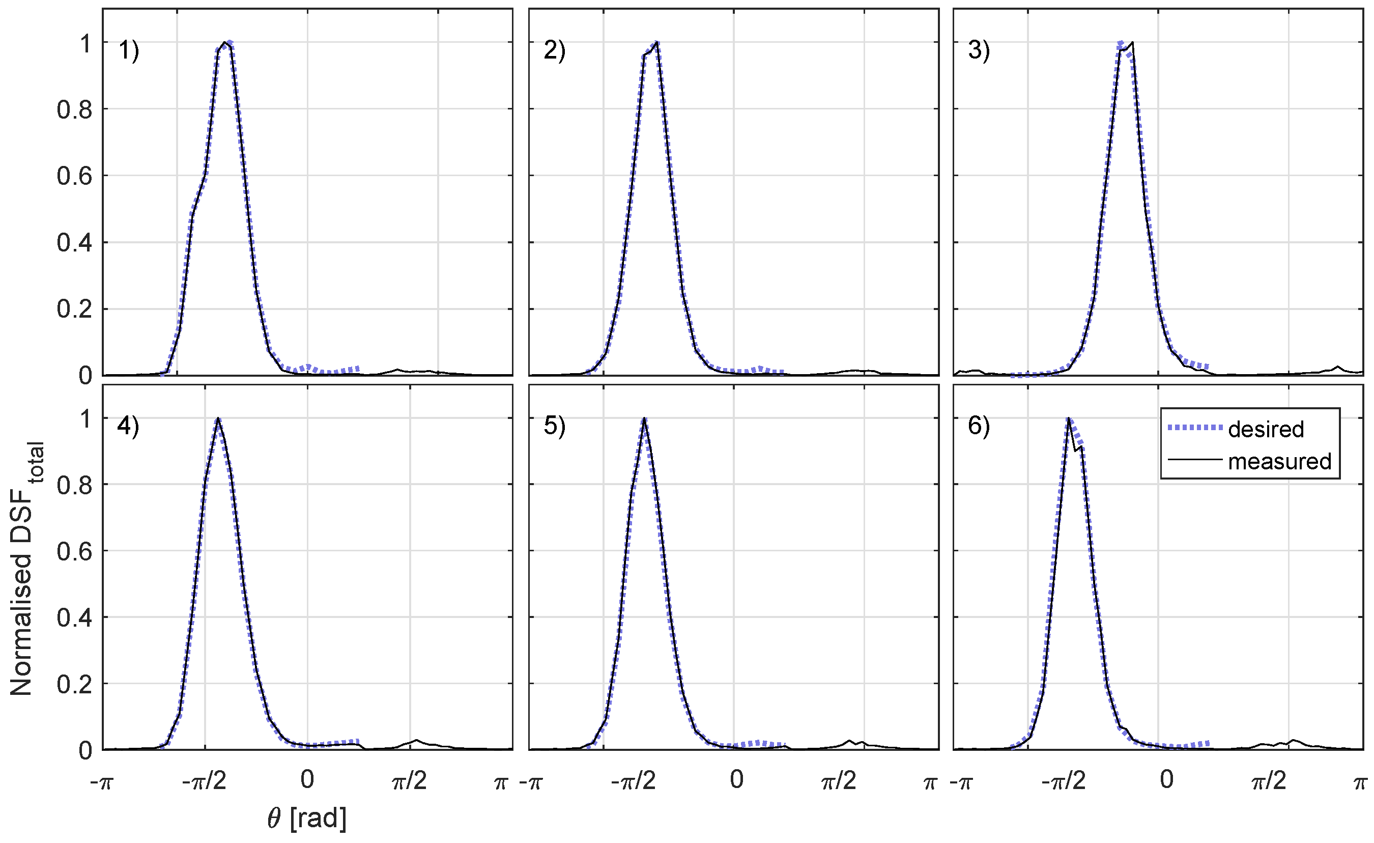
Figure 12.
SPAIR method directional spectrum outputs for the example extreme spectra. Total output directional spectra shown, including reflections. Energy densities are shown by the colour scale and are normalised by the maximum of the desired spectrum for each sea state. 1) to 6) correspond to sea states 1 to 6 defined in Table 1.
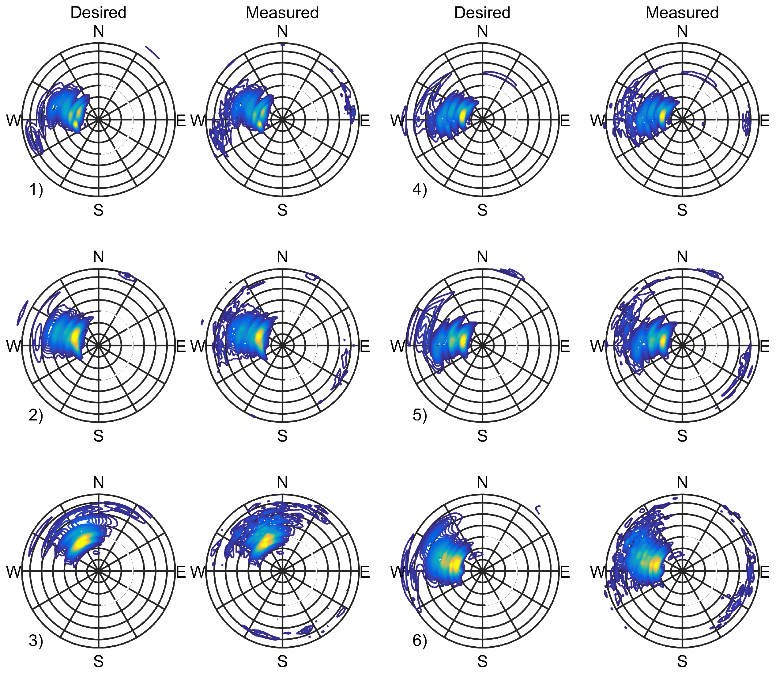
Figure 13.
Frequency spectra change for the three hours prior to the extreme sea state identified. 1) to 6) correspond to sea states 1 to 6 defined in Table 1.
Figure 13.
Frequency spectra change for the three hours prior to the extreme sea state identified. 1) to 6) correspond to sea states 1 to 6 defined in Table 1.
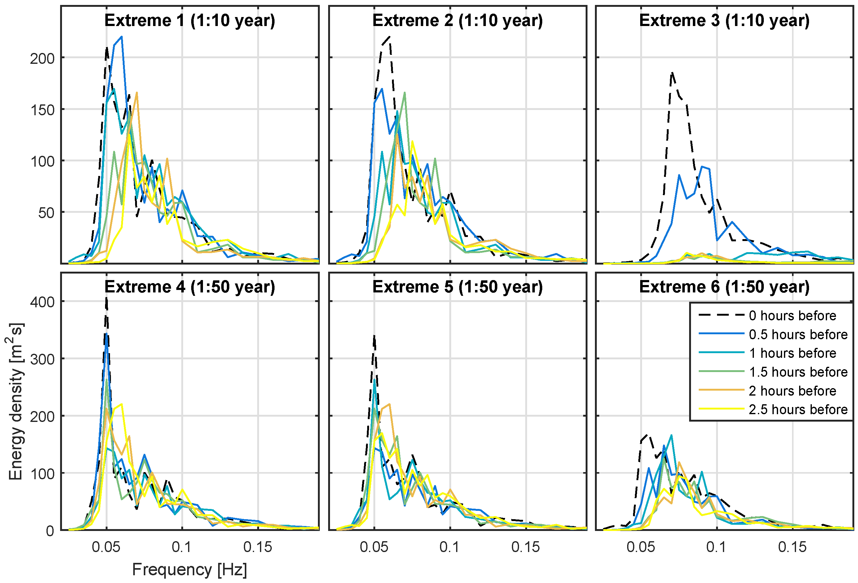
Figure 14.
Scatter diagram displaying identified example points for demonstrating spatial variability. Target values and observed values used for comparison are highlighted.
Figure 14.
Scatter diagram displaying identified example points for demonstrating spatial variability. Target values and observed values used for comparison are highlighted.

Figure 15.
Variation in frequency spectra and DSF’s for high example case. 17 spectra from 8 storms shifted onto the desired – target point 1 defined in Figure 14.
Figure 15.
Variation in frequency spectra and DSF’s for high example case. 17 spectra from 8 storms shifted onto the desired – target point 1 defined in Figure 14.
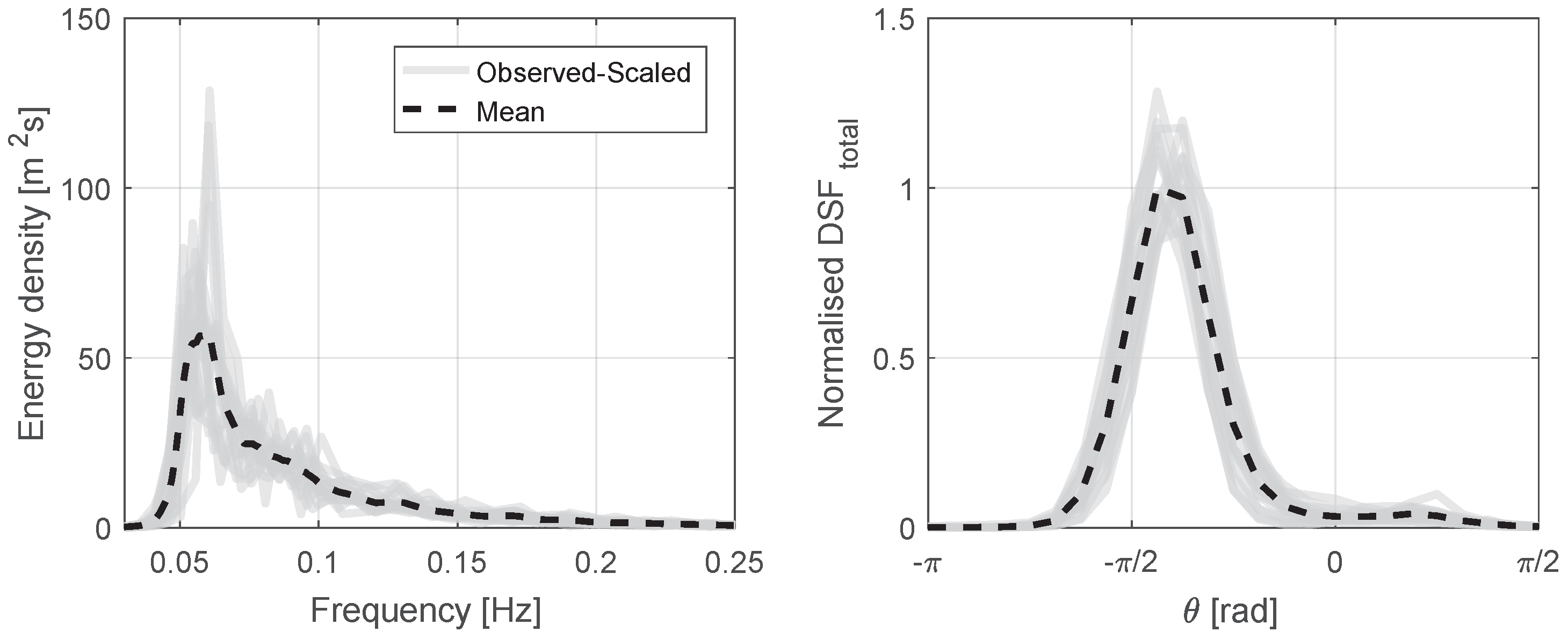
Figure 16.
Variation in frequency spectra and DSF’s for low example case. 33 spectra from 11 storms shifted onto the desired – target point 2 defined in Figure 14.
Figure 16.
Variation in frequency spectra and DSF’s for low example case. 33 spectra from 11 storms shifted onto the desired – target point 2 defined in Figure 14.


Table 1.
Example extreme – combinations for 1:10 and 1:50 year conditions.
| Extreme Sea State | 1 (1:10) | 2 (1:10) | 3 (1:10) | 4 (1:50) | 5 (1:50) | 6 (1:50) |
|---|---|---|---|---|---|---|
| 10.65 | 11.05 | 10.01 | 11.45 | 11.86 | 11.02 | |
| 15.21 | 14.78 | 11.86 | 16.61 | 16.32 | 12.66 |
Table 2.
Effect of various scaling approaches on other parameters (guaranteed Froude scaled parameters shown in blue).
Table 2.
Effect of various scaling approaches on other parameters (guaranteed Froude scaled parameters shown in blue).
| Scaling | Scaling | Scaling | |
|---|---|---|---|
| f | |||
| k | |||
© 2017 by the authors. Licensee MDPI, Basel, Switzerland. This article is an open access article distributed under the terms and conditions of the Creative Commons Attribution (CC BY) license (http://creativecommons.org/licenses/by/4.0/).
Share and Cite
MDPI and ACS Style
Draycott, S.; Davey, T.; Ingram, D.M. Simulating Extreme Directional Wave Conditions. Energies 2017, 10, 1731. https://doi.org/10.3390/en10111731
AMA Style
Draycott S, Davey T, Ingram DM. Simulating Extreme Directional Wave Conditions. Energies. 2017; 10(11):1731. https://doi.org/10.3390/en10111731
Chicago/Turabian StyleDraycott, Samuel, Thomas Davey, and David M. Ingram. 2017. "Simulating Extreme Directional Wave Conditions" Energies 10, no. 11: 1731. https://doi.org/10.3390/en10111731
Note that from the first issue of 2016, this journal uses article numbers instead of page numbers. See further details here.