A Transient Stability Numerical Integration Algorithm for Variable Step Sizes Based on Virtual Input


College of Electrical Engineering, Zhejiang University, Hangzhou 310027, China
*
Author to whom correspondence should be addressed.
Energies 2017, 10(11), 1736; https://doi.org/10.3390/en10111736
Submission received: 26 September 2017
/
Revised: 21 October 2017
/
Accepted: 26 October 2017
/
Published: 30 October 2017
Abstract
:In order to reduce the online calculations for power system simulations of transient stability, and dramatically improve numerical integration efficiency, a transient stability numerical integration algorithm for variable step sizes based on virtual input is proposed. The method for fully constructing the nonhomogeneous virtual input for a certain integration scheme is given, and the calculation method for the local truncation error of the power angle for the corresponding integration scheme is derived. A step size control strategy based on the predictor corrector variable step size method is proposed, which performs an adaptive control of the step size in the numerical integration process. The proposed algorithm was applied to both the IEEE39 system and a regional power system (5075 nodes, 496 generators) in China, and demonstrated a high level of accuracy and efficiency in practical simulations compared to the conventional numerical integration algorithm.
1. Introduction
The transient stability of a power system refers to the ability of a power system to regain its original state or achieve a new stable state after it has been suddenly subjected to an extreme disturbance in a given operating state. In transient stability simulations, the existence of numerous nonlinear equations limits the methods that can be used for this purpose. Since the 1990s, with the development of computing methods for matrix equations, real improvements have been made in the domain of differential equation calculations. The precise time step integration proposed by Zhong [1,2,3] is increasingly used in dynamic structural analysis. The precise time step integration has very high accuracy, and the calculation process is more stable, which makes the method superior in solving nonlinear dynamic differential equations.
However, precise time step integration will introduce calculation errors into the calculation of the inverse matrix, which requires a full rank matrix. When considering the use of precise time step integration in transient stability analysis, it is inevitable that even if the precise solution is used, it brings the problem of numerical instability to the algorithm itself. Given the applications of all kinds of quick regulating devices in a power system, the above problem may seriously affect the application of precise time step integration in transient stability simulations. Because the matrix inversion implies a disadvantage in the application and numerical stability of the numerical algorithm, large numbers of studies have been carried out on the precise time step integration method without matrix inversion. The increment dimensional method is a modified approach for precise time step integration [4,5,6]. The basic principle is to treat the nonhomogeneous term as a state variable of the dynamic equation by increasing the dimensions, so the nonhomogeneous dynamic equation can be transformed into a homogeneous dynamic equation. This method avoids the matrix inversion in the calculation process, and it is better than the conventional algorithm in general. However, when the number of dimensions is too high, there will be problems, such as the curse of dimensionality. The parallel algorithm based on the high precision direct integration method is presented and evaluated [7,8,9]. In reference [7], an integration scheme is derived by distinguishing the rigid-body modal. This parallel algorithm improves the calculation efficiency and the stability of precise time step integration. The authors of [8] present a parallel algorithm. A mixed fine grain and coarse grain strategy for parallel computing is developed. A hybrid form involving two types of coarse parallelization is also shown to have advantages when a Fourier series form of the high precise direct method is used. The authors of [9] propose a parallel high precision integration based on matrix exponential and time domain segmentation for solving the semi-discretized system by SEM. It is very suitable for long time simulation and can achieve accuracy several orders higher than that of conventional time stepping methods such as the Runge-Kutta schemes. The authors of [10] extend high precise direct scheme to analyses systems with loading or impact, through Fourier expansion and homogenizing the initial system. Compared with other methods, the new scheme named homogenized high-precision direct integration has a higher precision and wider application. The authors of [11] propose a new efficient and high precision direct integration scheme based on 2N type algorithm for the computing of exponential matrix. The study demonstrates that precise integration method can be effectively applied to nonlinear numerical analysis of rotor-seal system. The scheme is significantly less sensitive to the size of time step compared with other existing methods, so a large time step may be used and the computing time reduced substantially. The generalized precise time step integration method proposed by professor Fu [12] uses Taylor series expansion, and skilfully makes use of the transfer function matrix formed in each integration subinterval. The method greatly reduces the matrix multiplication times introduced by direct expansion, and the truncation error is still introduced by the homogeneous method. The natural computational advantage renders it the best precise time step integration method for calculating nonlinear nonhomogeneous equations, and it is quite suitable for transient stability simulations.
Existing studies have already introduced precise time step integration into transient stability simulations for power system. The authors of [13] used an algorithm of the factors table based on precise time step integration to avoid the inverse matrix calculation, and proposes a fast power system dynamic simulation method, which reduces the number of calculations and has improved computational stability. The author of [14] proposed an implicit precise integration method based on Duhamel integration. The calculation speed can be improved to some extent, while the calculation accuracy for power angle is not improved significantly. The author of [15] presented a high-precision, high efficiency precise time-integration method based on multi-step prediction. The multi-step prediction polynomial fitting of nonlinear part is used in this method. However, the systematic construction method for the nonlinear part is not given, and the multi-step construction for the transient stability simulation is not presented in detail. The authors of [16] presented a novel time-domain integration method for transient analysis of non-uniform multi-conductor transmission lines. In order to eliminate the Courant-Friedrich-Levy condition constraint, a precise time-step integration method is utilized in time-domain calculation. The proposed method has the superiority of calculation accuracy and stability. Considering the applications to transient stability simulations, relevant studies have made great achievements, although they have some shortcomings also. First, the existing studies only give a relatively concrete integration scheme when proposing an algorithm based on precise time step integration. However, a systematic and complete construction method for arbitrary accuracy is not given. Additionally, when analysing the accuracy for the algorithm, only the accuracy of the transfer matrix is analysed, and the accuracy of the generator state variable is not analysed. Second, the use of a larger integration step size is a strong advantage in precise time step integration. Existing algorithms all use a unified step size, which does not take advantage of the high accuracy and convergence characteristics of the precise time step integration. Moreover, the scale of the cases used in the existing studies is so small that the actual effect of the algorithm in applications with a large-scale power system and engineering practices cannot be fully shown.
In light of these problems, and based on generalized precise time step integration, a new numerical integration algorithm for variable step sizes based on virtual input is proposed. In this study, the idea of virtual input is presented, and the systematic construction method for vitual input is given. The local truncation error of the power angle for the corresponding integration scheme is derived. Then, a step size control strategy based on the predictor-corrector variable step size method is proposed, realizing adaptive control of the step size in the numerical integration process. The whole procedure for the proposed algorithm is presented, at the same time, a practical large-scale power system is used to demonstrate the proposed algorithm. The rest of the paper is organized as follows: In Section 2, the new algorithm is presented in detail. Section 3 presents the concrete form of the differential equations. Section 4 shows the integration step size adaptive control strategy. Section 5 presents the limiting link process and gives the whole procedure for the algorithm. Section 6 presents a case study and discusses the results thus obtained. Section 7 provides concluding remarks for the paper.
2. Transient Stability Numerical Integration Based on Virtual Input (VII)
Differential equations for power systems can be expressed as:
Since the analytical solutions of nonlinear differential equations cannot be obtained, a linear term and a nonlinear term are separated from . Thus, Equation (1) can be expressed as:
where is a constant matrix, and . here is a nonlinear function of the simulation time, state variables, and operational variables.
On the premise that is a constant matrix, in the integral interval , the analytic high-order function that has the form of Equation (6) is used to fit the nonhomogeneous term, the coefficients of which are constructed using the value of at time and as shown in Equation (10). The nonhomogeneous term of this construction method is defined as the “virtual input”.
According to control theory, the scheme of the virtual input can directly influence the dynamicresponse of the nonlinear system, and based on the virtual input, a transient stability numerical integration algorithm is proposed in this paper.
The state variable at time is known as ; and thus the state variable at the time is:
Equation (3) can be expressed as:
where is the homogeneous solution of the differential equation, and is the nonhomogeneous solution. For the nonhomogeneous solution, a high-order function is used to fit during the integration interval so that the real value can be approximated to the maximum, that is:
and Equation (6) can be substituted into Equation (5):
First, calculate the integration value of each order function in the nonhomogeneous solution (see Appendix A):
In the derivation of Equation (8), is expanded into the power series:
Second, use the value and of the at time and to construct in the implicit scheme:
In Equation (10), there is (see Appendix B):
Then, take the quadratic function as an example to construct the virtual input, and the concrete numerical integration scheme and the highest calculation accuracy of the power angle can be calculated. Substitute Equation (11) into Equaiton (10):
Since the matrix (the concrete form will be explained in detail) possesses the quantitative relation , this means that the power angle line is a zero vector in the high-order power of matrix , and the product of the high-order power of matrix and the state variable vector is the zero vector. Therefore, Equation (8) can be simplified by omitting the high-order term:
For the power angle , the product of Equations (12) and (13) is equal to that of Equations (8) and (12). Multiply Equations (12) and (13):
Substituting Equation (14) into Equation (7), is obtained. Then, the final form of Equation (4) is:
In the derivation of Equation (15), is simplified by omitting the high-order term as Equation (16) because the product of the high-order power of matrix H and the state variable vector is the zero vector:
Since , there is . For the power angle , Equation (15) can be translated into Equation (17):
On the other hand, according to the Taylor series expansion, is:
The configuration of Equation (10), that is, the values of , determine the accuracy of power angle for the constructed scheme. If the sixth-order is the reached, the coefficient of each term in Equations (17) and (18) should be equal. The undetermined coefficients’ equation system can be obtained:
It is worth noting that the equation system has infinite solutions if the first six equations are considered, while it has no solution when the rest of the equations are considered. Thus, it can be found that the calculation of the power angle can reach fifth-order accuracy when the quadratic function is used to fit the virtual input, and the principal local truncation error is . A set of solutions is given as:
that is:
In a similar way, the calculation of the power angle can reach third-order accuracy when the linear function is used to fit the virtual input, and the principal local truncation error is . A set of solutions is given as:
that is:
The calculation of the power angle could reach third-order accuracy when the constant is used to fit the virtual input, and the principal local truncation error is . The unique solution is given as:
that is:
It should be noted that a function could also construct an integration scheme of relatively lower accuracy. For example, the quadratic function could also construct an integration scheme at the fourth order. In addition, it is observed that the high-order derivative of the generator state variables must be calculated when an integration scheme is constructed for which accuracy exceeds the third order. The author of [17] gives the derivation process of the derivative of the power angle. It relies on the derivative of bus node voltages when the complicated generator model is applied, and it can only be calculated by solving the network equations. This is hard to apply to fast transient stability simulation, as it concentrates on computing speed. On the other hand, the derivative of state variables can be calculated by a difference quotient instead of a differential quotient, using the multi-step method. However, using the difference quotient of the numerical result from the forward step and backward step directly in a large step size cannot assure accuracy, and many additional calculations for differential algebraic equations are introduced if the large step is divided into small ones, which seriously influences the computing speed. Thus, in practical application, the constructed integration scheme generally has lower than third-order accuracy.
After constructing a virtual input at a certain accuracy, define as:
Because the integration interval of a homogeneous item continuously extends in the form of the power of 2, the calculation equation of from a small integration interval to should be derived after the step size is elaborated:
Let
Substitute Equation (22) into Equation (21):
The final integration equation for the state variable is:
where is calculated by precise time step integration, and no further details are given here.
3. Concrete form for the Differential Equations
The sixth-order generator model is applied, for which there is change. The differential equations for the model are:
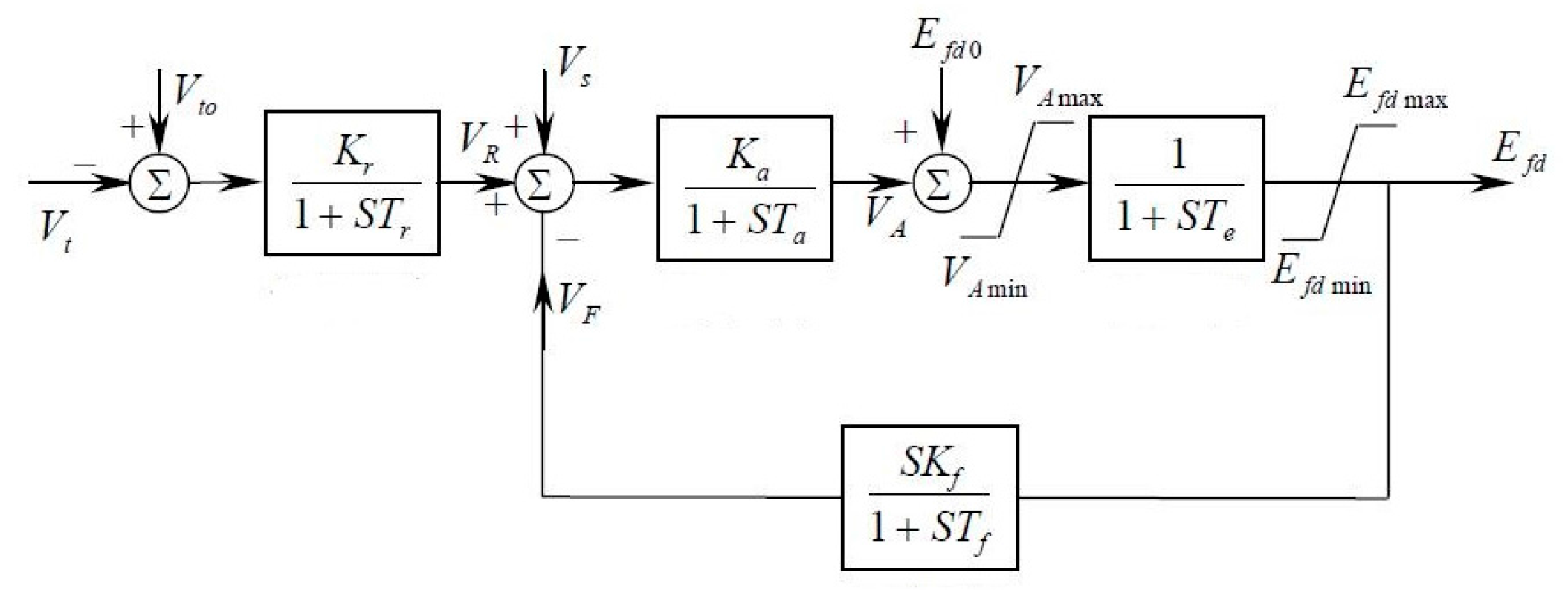
A conventional or fast excitation system and thyristor regulator are applied, and the simulation construction is shown in Figure 1.
The differential equations for the variables are the following:
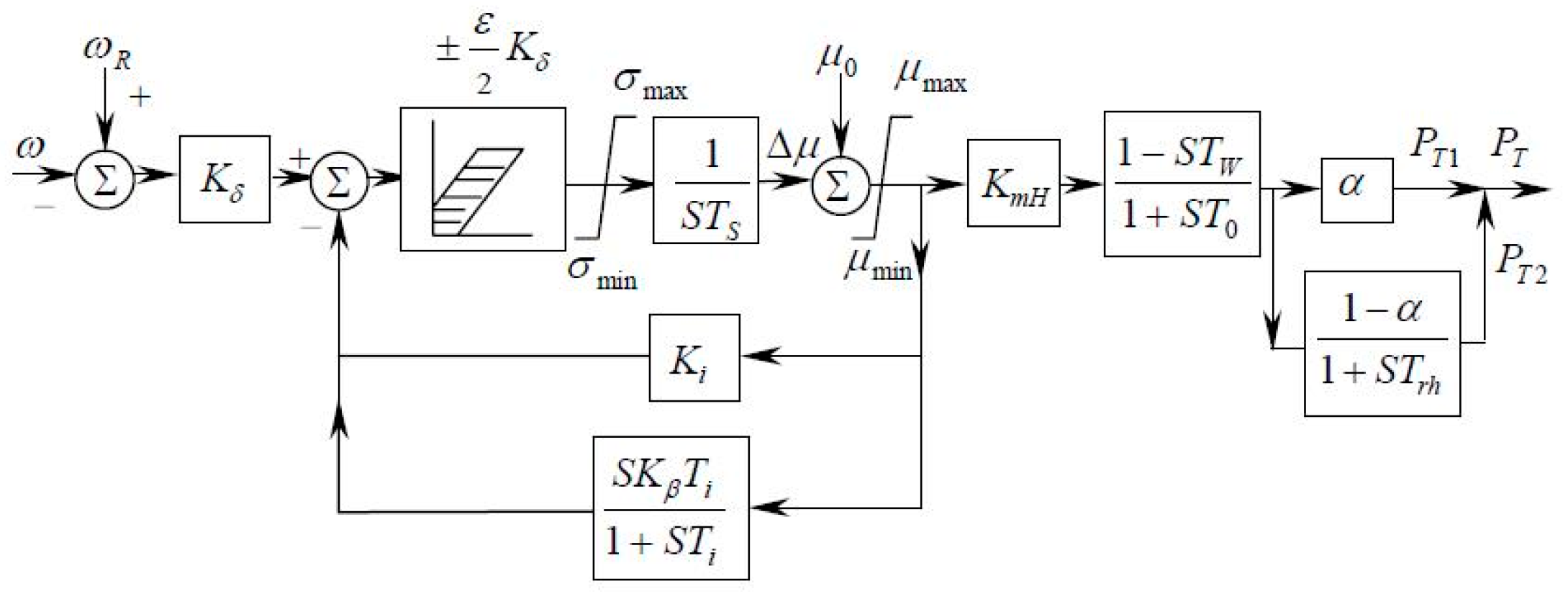
A universal governor model that is applicable to hydropower generating units and thermal power generating units is applied, and this model includes the measurement part, distributing valve, servosystem, feedback loop, water hammer effect, and generator reheating regulator. The simulation construction is shown in Figure 2.
The differential equations for the variables are as follows:
The differential equations for the generator rotor, exciter, and governor above constitute all of the differential equations for transient stability analysis. The constant matrix H and virtual input separated from the differential equation system are shown in Figure 3. The reason for putting , which contains a state variable, into the virtual input is that the saturation coefficient will change in every iteration, assuring that H is a constant matrix so that the calculation of the transfer matrix can be fully completed offline without the costs of online simulation time.
4. Integration Step Size Adaptive Control Strategy
Because the solutions of stiff problems have rapidly varying components and slowly varying components, a small step size should be applied when the solution changes rapidly, and a large step size should be applied when the solution changes slowly. Besides, in considering self-starting, a small step size is applied at the beginning of the simulation, and then, the step size may be adjusted appropriately to obtain the optimal step size as the simulation goes forward. The optimal step size here is taken to mean that the amount of computing is minimized while the solution satisfies the given accuracy.
The local truncation error is estimated using the difference value of the explicit Euler predictor and high-order corrector proposed in this paper. Supposing that the power angle calculated by the explicit Euler predictor at time is , there is:
Supposing that the corrector has the highest accuracy of order, and the power angle calculated by the corrector at time is , there is:
Substituting Equation (28) into Equation (29):
The step size could be adjusted according to the value calculated by Equation (30) so that the local truncation error can stay near the maximum permissible error. For an integration scheme of third-order accuracy with the virtual input fitted by the linear function, the local truncation error of the power angle at time is proportional to the fourth-order power of the step size. If the maximum permissible error is , the updating equation for the step size is:
where is the previous step size. An advantage of using precise time step integration to calculate the transfer matrix is that when knowing all the parameters of the generators, the full calculations can be completed offline. Take 0.01 s as the basic step size. The transfer matrix can be calculated for all the possible step sizes. The updating equation of step size can be improved to:
where is the integral function. In this way, all of the possible transform matrixes can be calculated offline and the step size avoids being updated too frequently.
5. Variable Step Size Transient Stability Numerical Integration Algorithm Based on Virtual Input (VSVII)
5.1. Process for Nonlinear Links
There are many nonlinear links such as the output limiting link, the dead time in the transient stability simulation, the exciter and governor introduced in Section 3 for instance. In practical engineering applications, the number of such nonlinear links is enormous for a large power system with hundreds of generators. In the conventional process for such links, the exact time when the state variables would reach the limiting value is calculated and the present result would be abandoned. Then, the simulation goes back to the previous time step and recalculates to the limiting time using the functions for the limiting case. Although this method is very accurate for a large power system, the backoff calculations cost too much time, and are more significant than using a large step size.
The algorithm in this paper applies the following method. For a certain state variable and its limiting values (or ), a limiting control interval is set. The step size is decreased if the value of the state variable falls into the control interval, and the simulation goes with a small step size. When the state variable reaches its limiting value , the function for the limiting case and a large step size are applied. Although the method cannot ensure that the limiting link is exactly calculated, by adjusting the limiting interval range, excessive back-off calculations can be avoided while guaranteeing a certain accuracy, which significantly reduces the additional calculations, and this is especially suitable for transient stability simulations of a large-scale power system.
5.2. Simulating Procedure for the VSVII Algorithm
The full simulation procedure for VSVII is presented as follows:
- Step 1:
- Input all the information for the power system, and proceed to power flow calculation to obtain the operational variable values for the stable state, including bus node voltage , injection current to the network, and electromagnetic power .
- Step 2:
- Calculate the initial value of the state variables, including the power angle , angular frequency , transient and sub-transient electromotive force (EMF) of the generators, and all the initial values for the exciters and governors.
- Step 3:
- Form the differential equations and network algebraic equations describing the transient process of the power system, and form the factors table.
- Step 4:
- Set the initial calculation time for transient stability .
- Step 5:
- Check if a fault occurs; if so, proceed to step 6. If not, proceed to Step 8.
- Step 6:
- Modify the network algebraic equations and the factors table according to the faults and operations.
- Step 7:
- Solve the network algebraic equations and obtain the new values for the operational variables.
- Step 8:
- Calculate the values of the state variables at time including the power angle , angular frequency , transient and sub-transient EMF of the generator, and all the values for the exciter and the governor. Calculate the values for the operational variables including bus node voltage , injection current for the network, and electromagnetic power . The steps in the process in detail are as follows:
- Step 8.1:
- Update the step size according to the process for limiting links in Section 5.1 and the step size control strategy in Section 4. Check if the step size obtained is the same as the previous size. If so, proceed to Step 8.3. If not, proceed to Step 8.2.
- Step 8.2:
- Call the state transfer matrix and calculated offline. Calculate for each order in the nonhomogeneous term using the values of the state variables and operational variables at time and calculate the values of the state variables at time using Equation (24).
- Step 8.3:
- Set the iteration time .
- Step 8.4:
- Calculate the values of the operational variables using the network equation and the values of the state variables obtained.
- Step 8.5:
- Update the value in using the new values for the operational variables obtained. Calculate the new values for the state variables.
- Step 8.6:
- Check the maximum difference value of the power angle for each generator between two iterations. If the value is greater than the given precision, set and go back to Step 8.4. Otherwise, proceed to step 9.
- Step 9:
- The simulation goes on to the next step; set .
- Step 10:
- If , go to step 11. Otherwise, go back to Step 5.
- Step 11:
- The simulation is completed. Output the result.
6. Simulation and Results
First, the VSVII algorithm was applied to the IEEE39 system, the computer equipment used in the simulation comprised an Intel Core 2 CPU i3-2100, 3.10 GHz, with 8 GB of memory, equipped with the Windows 7 operating system.
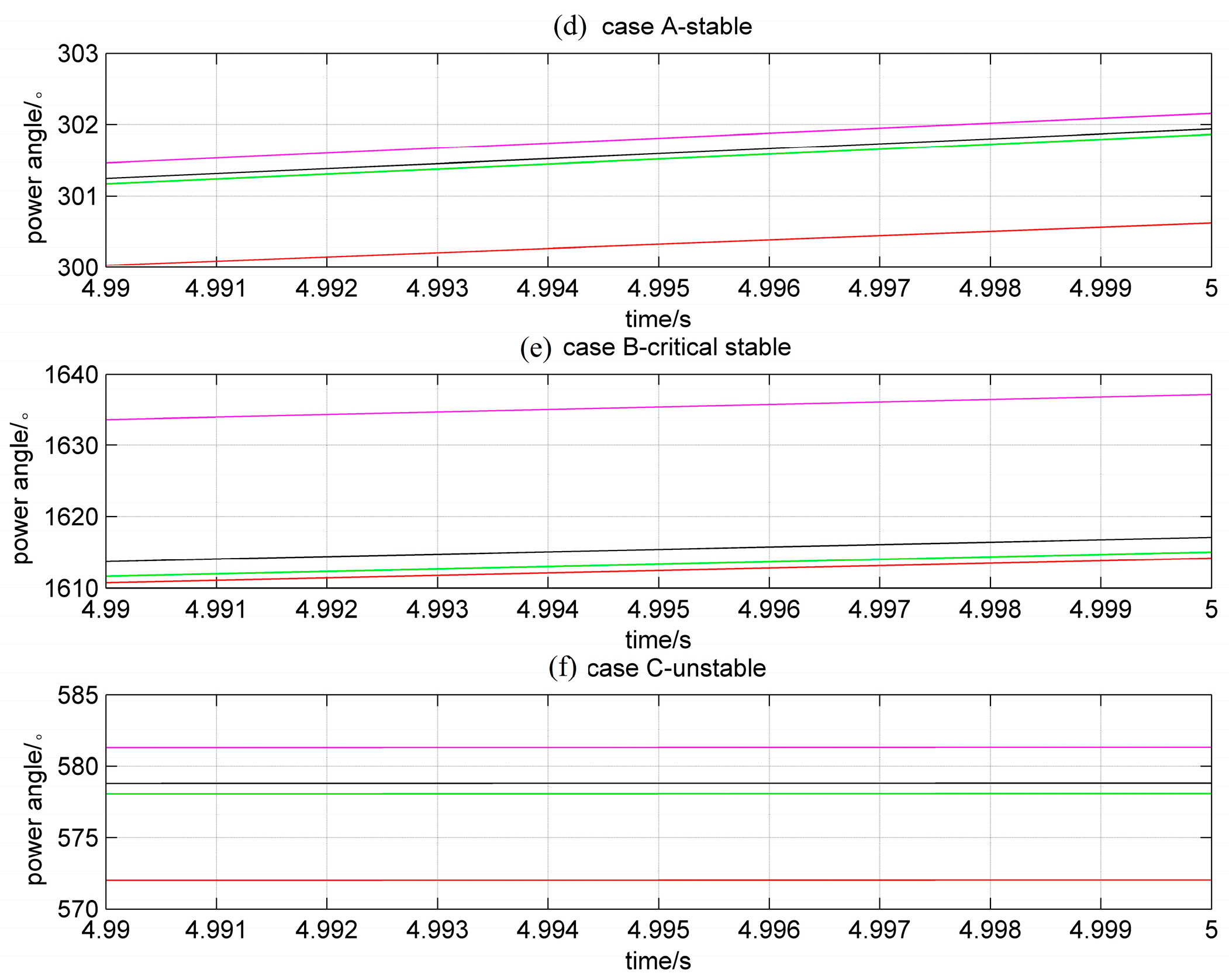
The study first focused on a comparison of the simulation results using the algorithms for VSVII, VII with third-order accuracy, and implicit trapezoidal integration (TI) to illustrate that VSVII and VII had the same simlation results as TI and the standard value, while reducing the amount of computing for the differential algebraic equations. A three-phase short circuit fault was set on line 35 (case A), line 9 (case B), and line 44 (case C) for 0.2 s, respectively, and then cut. The simulation result calculated by the synthesis program of the China Electric Power Research Institute (PSASP) using a step size of 0.001 s was regarded as the standard value. The step size for TI, VII and the initial step size for VSVII was 0.01 s. The simulation lasted for 5 s. If the maximum power angle difference in the simulation was not greater than 180 degrees, the power sytem had transient stability. In each case, the power angle of the same generator using different integration algorithms was observed, the curves of which are shown in Figure 4.
It can been seen from Figure 4 that the power angle curves calculated by VSVII and VII are consistent with TI and the standard value, illustrating the effectiveness of VSVII and VII. The main calculation of the transient stability analysis concentrates on the solution of differential equations and algebraic equations, which reflects the integrated performance of different algorithms. Table 1 gives the detailed numerical results, and it can be found that VSVII significantly reduces the amount of calculation for the differential algebraic equations, although there is no significant reduction for VII using a small step size compared with TI.
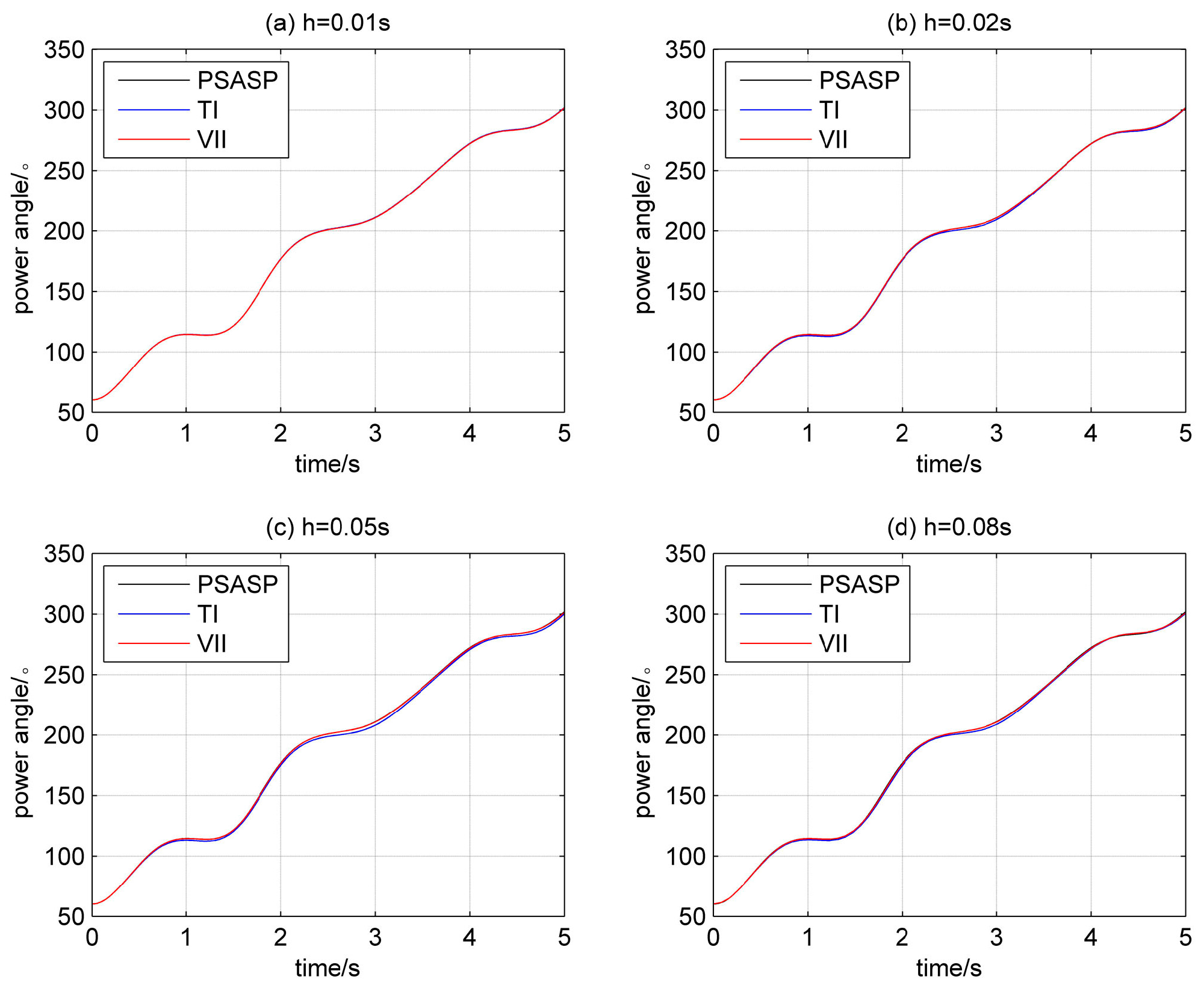
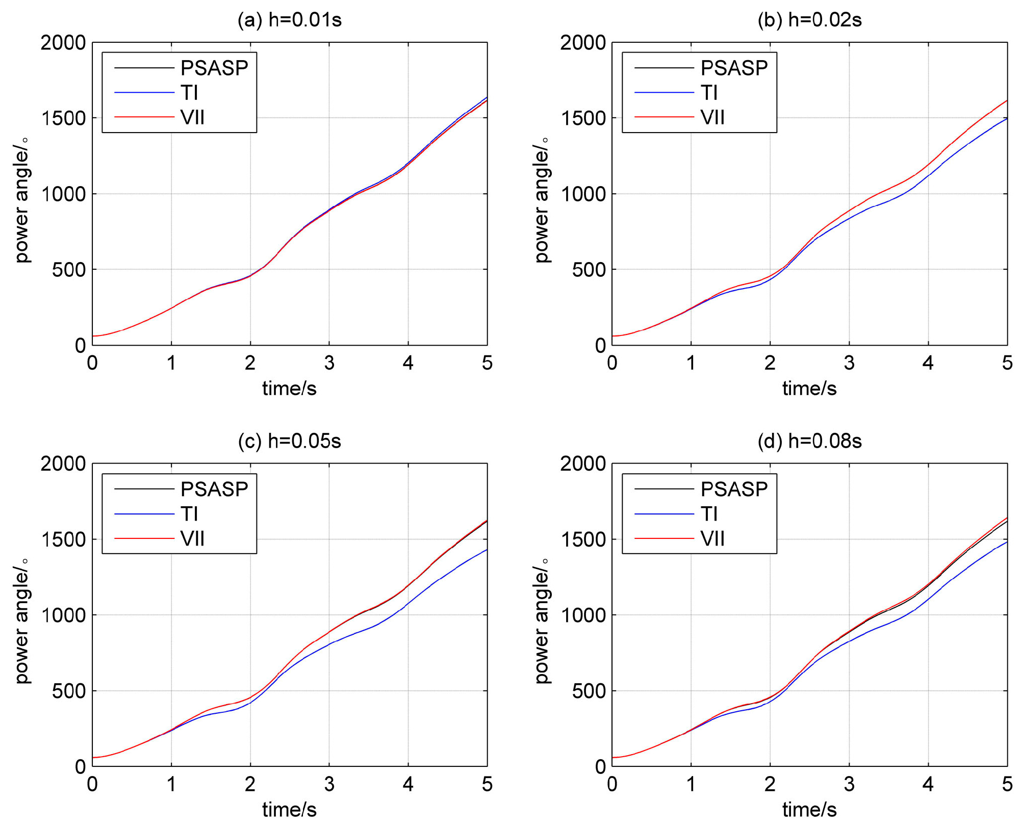
To analyze the superiority of VII using a large step size compared with TI, the numerical integation is performed using the step sizes of 0.01 s, 0.02 s, 0.05 s, and 0.08 s, respectively, in each case, and the simulation results are shown in Figure 5, Figure 6 and Figure 7. It can be seen that VII and TI have an approximate simulation accuracy using different step sizes in case A. In case B, VII has a high accuracy at the step sizes of 0.02 s, 0.05 s, and 0.08 s. In case C, VII has a high accuracy at the step sizes of 0.02 s, 0.05 s, and 0.08 s, but the power angle curve starts to appear different from the standard curve using the step sizes of 0.05 s and 0.08 s. Since the state variables for the differential equations change little with a small step size, the superiority of VII is not represented significantly. However, with a large step size, the accumulated error of TI gradually increases, while the accumulated error of VII is much smaller. By comparing the accuracy and amount of computation for VII and TI using a large step size (through Table 1 and Figure 5, Figure 6 and Figure 7), it is observed that VII significantly reduces the amount of computing for the differential algebraic equations, for which there is a more than 30% reduction, guaranteeing the required accuracy.
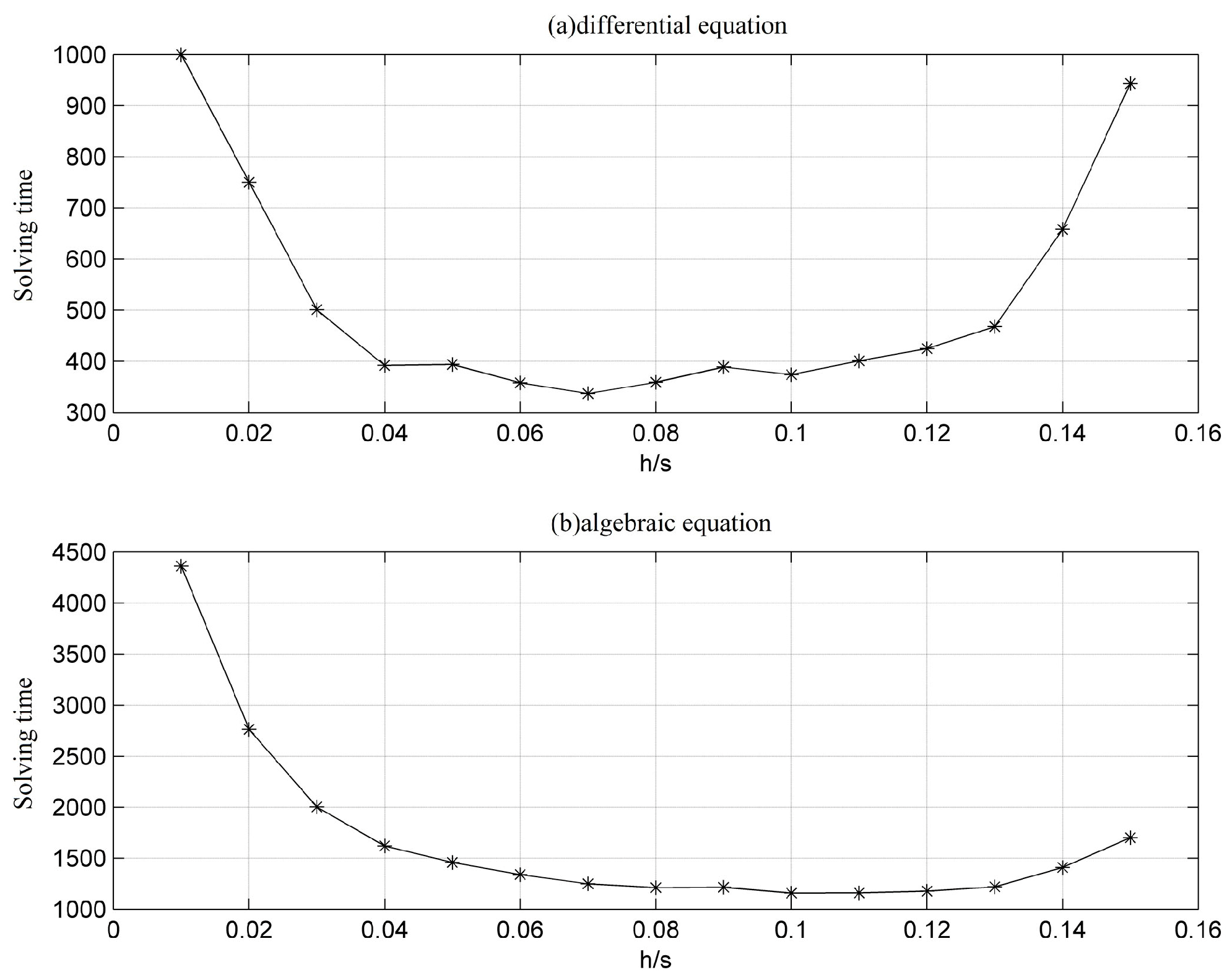
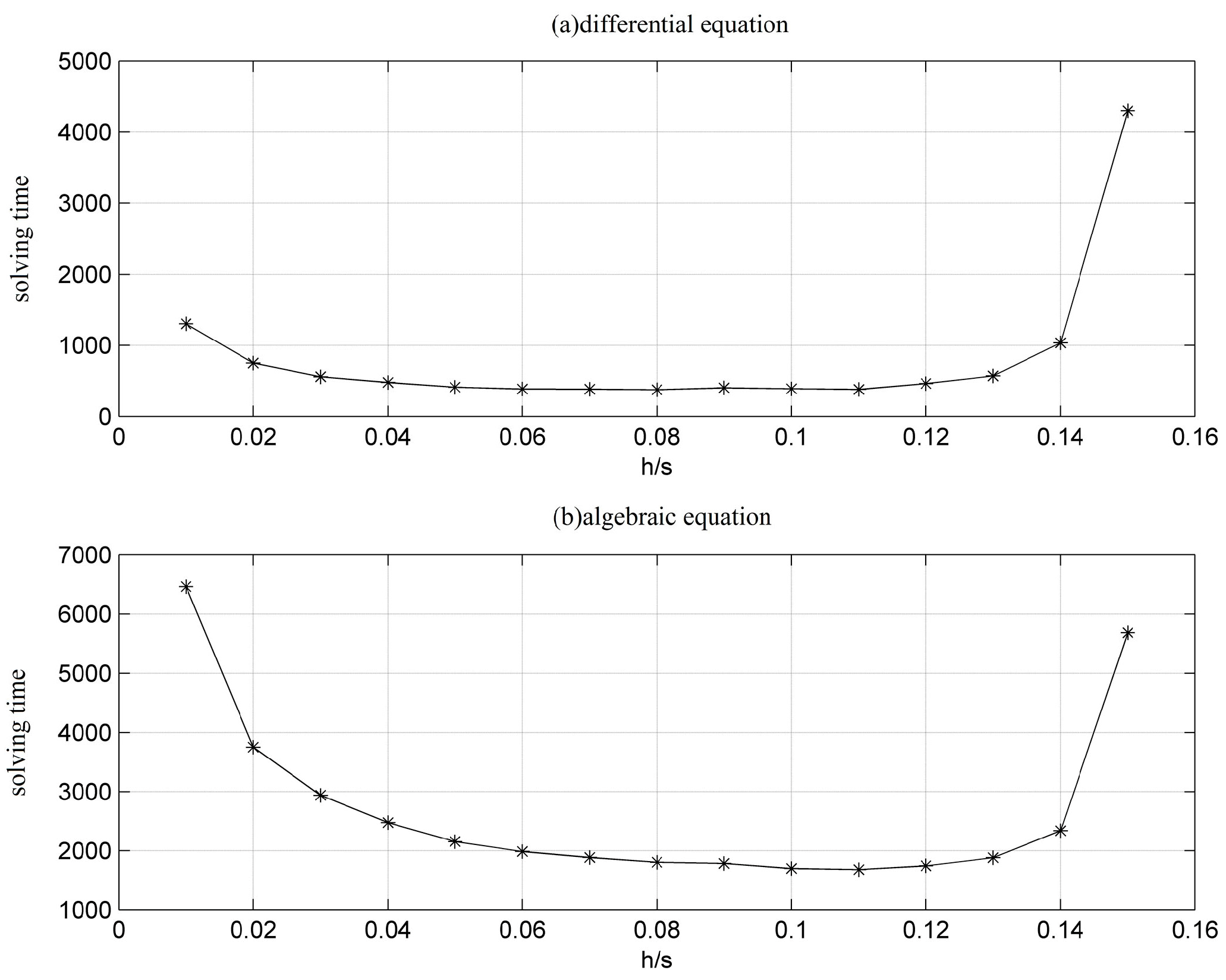
Since VII has the advantage of high accuracy and convergence, it has practical engineering significance in applying the algorithm using a large step size. The calculation accuracy of VII in different cases is not the same when observing the above cases. Furthermore, the optimal step size for different cases is not the same for analyzing the variations in the amount of computing for the differential algebraic equations as the step size changes in Figure 8, Figure 9 and Figure 10. It can be seen that the algorithm requires less computing for the differential equations using the step sizes of 0.06–0.10 s, and less computing for the algebraic equations using the step sizes 0.08–0.12 s. Considering the computing accuracy, VII still has high accuracy when using the step size of 0.08 s in case A and case B, and has a high accuracy using the step size of 0.05 s, which starts to reduce when using a step size greater than 0.05 s as compared to the standard value from PSASP in case C. Therefore, VSVII as proposed in this paper must adaptively control the variation in the step size in different cases, and save the volume of computing as much as possible while maintaining a certain level of accuracy.
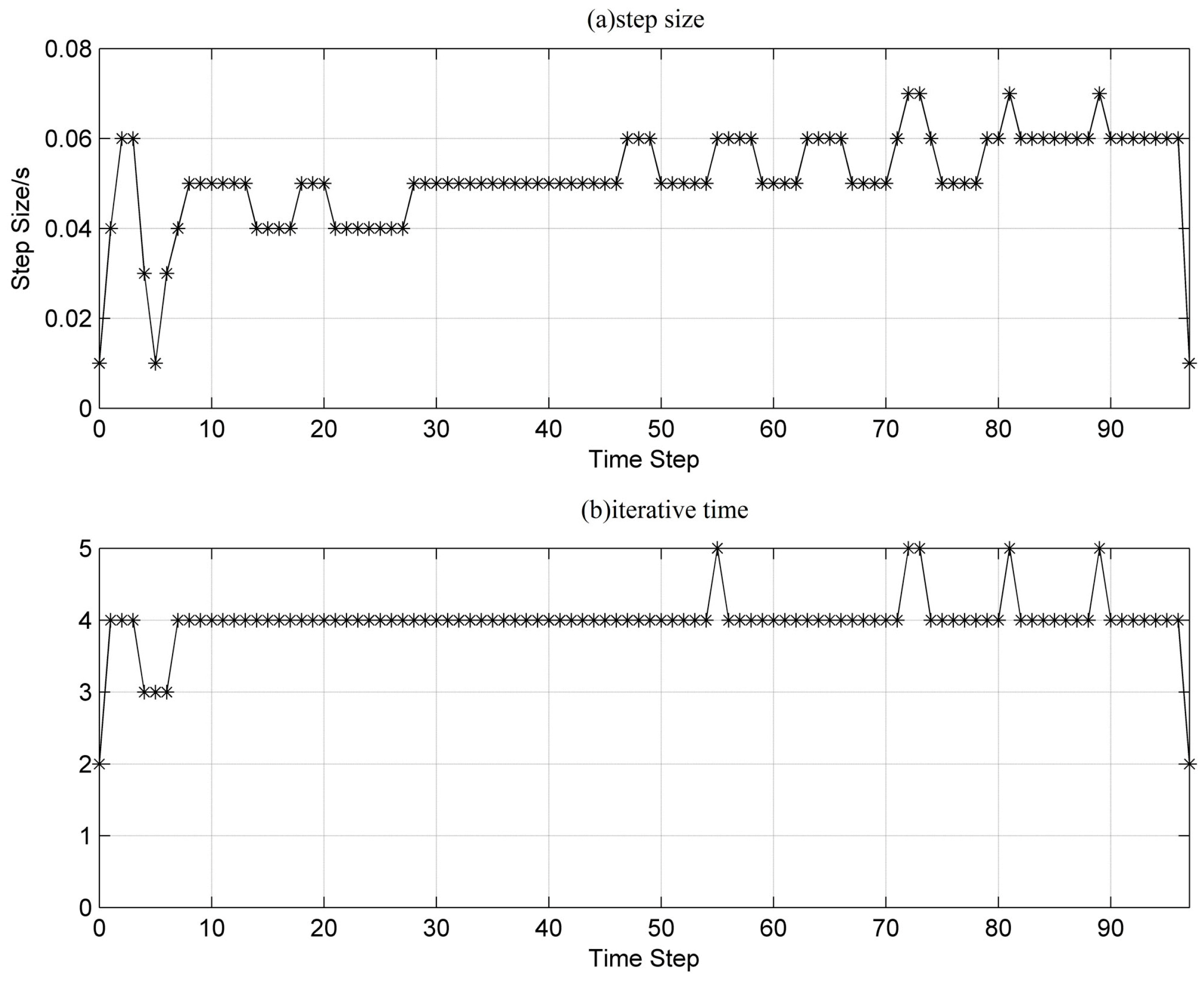
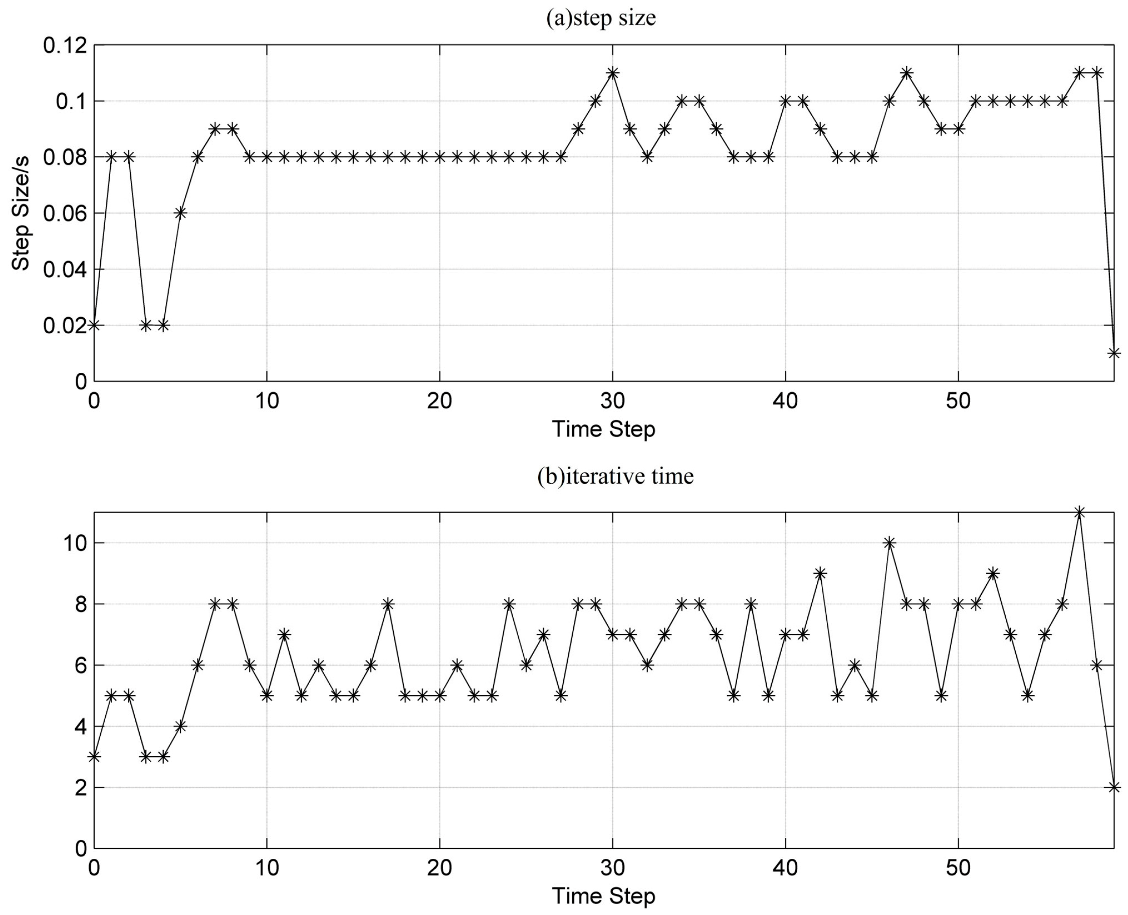
For the simulation of VSVII, the initial step size is set at 0.01 s, and the accuracy of the local truncation is controlled to . The variation in power angle is shown in Figure 4, and the detailed numerical results are shown in Table 1. Figure 11, Figure 12 and Figure 13 show the step size and the alternating iteration times at every time step for each case. The step size is generally maintained within 0.08 s–0.11 s in case A, 0.05 s–0.07 s in case B, and 0.04 s–0.06 s in case C. From the previous analysis, the step size determined can guarantee the calculation accuracy and reduce the total amount of computing. Though the total amount of computing can be further reduced using an even larger step size, the required accuracy cannot be satisfied. In general, the amount of computing for differential algebraic equations can be reduced by more than 60% using VSVII compared to VII with a constant step size of 0.01 s. Because the calculations for the transfer matrix can be fully completed offline, the computing time can be reduced by about 50%, as seen in Table 1.
Finally, VSVII was applied in a regional power system in China to verify the viability for large-scale power systems. The regional power system contained 496 generators and 5075 computational nodes. Generator models of type 0, type 2, and type 6, the constant impedance load, the exciter in Figure 1, and the governor in Figure 2 were applied. The simulation lasted for 5 s, and the initial step size for VSVII was 0.01 s. The step size for TI as a contrast is 0.01 s. Three sets of faults were set respectively to make the system stable, reach a critical state, and become unstable, and detailed simulation results are given in Table 2. It can be seen that the algorithm proposed in this paper can obtain an accurate simulation result and reduce the amount of computing. It is worth mentioning that because of using the system itself, the step size during simulation was not greater than 0.03 s. The computing time was reduced by 15% or so.
7. Conclusions
A transient stability numerical integration algorithm for variable step sizes based on virtual input is proposed in this paper. The method for constructing the nonhomogeneous virtual input in a certain integration scheme is given fully, and the calculation method for the local truncation error for the power angle is derived. A step size control strategy based on the predictor corrector variable step method is proposed, performing an adaptive control of the step size. The algorithm is applied in the IEEE39 system and in a regional power system in China (5075 nodes, 496 generators), showing the high precision and high efficiency of the algorithm in practical engineering simulations.
At the same time, the following directions will be further investigated at the next stage:
- (1)
- The accuracy estimation method for all the generator state variables will be derived to better control the numerical integration process.
- (2)
- The algorithm scheme will be completed for all the mathematic models of the real generators and regulators, more than the models introduced in this paper.
Author Contributions
Jianquan Wang conceived and designed the research; Yifan Gao performed the research, simulation and wrote the paper; Tannan Xiao analyzed the data and Daozhuo Jiang made suggestions on review.
Conflicts of Interest
The authors declare no conflict of interest.
Appendix A. Verification of Equation (8)
Appendix B. Verification of Equation (11)
Apply Taylor series expansion to
On the other hand, from the relation between , and , there is:
Subsitituting (A3) into (A2):
Taking the derivative of the two-sides of Equation (A4):
References
- Zhong, W.X. On precise integration method. J. Comput. Appl. Math. 2004, 163, 59–78. [Google Scholar]
- Zhong, W.X.; Williams, F.W. A precise time step integration method. J. Mech. Eng. Sci. 1994, 208, 427–430. [Google Scholar] [CrossRef]
- Zhong, W.X.; Zhu, J.P.; Zhong, X.X. A precise time integration algorithm for non-linear systems. In Proceedings of the Third World Congress on Computational Mechanics (WCCM-3), Chiba, Japan, 1–5 August 1994; pp. 12–17. [Google Scholar]
- Gu, Y.X.; Chen, B.S.; Zhang, H.W.; Guan, Z.Q. Precise time-integration method with dimensional expanding for structural dynamic equations. AIAA J. 2001, 39, 2394–2399. [Google Scholar] [CrossRef]
- Fung, T.C.; Chen, Z.L. Precise time-step integration algorithms using response matrices with expanded dimension. AIAA J. 2008, 46, 1900–1911. [Google Scholar] [CrossRef]
- Huang, Y.Z.; Long, Y.J. On orthogonal polynomial approximation with the dimensional expanding technique for precise time integration in transient analysis. Commun. Nonlinear Sci. Numer. Simul. 2007, 12, 1584–1603. [Google Scholar] [CrossRef]
- Lin, J.H.; Shen, W.P.; Williams, F.W. A high precision direct integration scheme for structures subjected to transient dynamic loading. Comput. Struct. 1995, 56, 113–120. [Google Scholar] [CrossRef]
- Shen, W.P.; Lin, J.H.; Williams, F.W. Parallel computing for the high precise direct integration method. Comput. Method Appl. Mech. Eng. 1995, 126, 315–331. [Google Scholar] [CrossRef]
- Huang, Y.Q.; Jie, F.; Zhang, J.Z.; Liu, Q.H. A parallel high precision integration scheme with spectral element method for transient electromagnetic computation. In Proceedings of the 14th Biennial IEEE Conference on Electromagnetic Field Computation, Chicago, IL, USA, 9–12 May 2010. [Google Scholar]
- Wang, J.; Tian, X.; Zhou, G. Homogenized high precision direct integration scheme and its applications in engineering. Commun. Numer. Methods Eng. 2002, 18, 429–439. [Google Scholar] [CrossRef]
- Hua, J.; Swaddiwudhipong, S.; Liu, Z.S.; Xu, Q.Y. New high precision direct integration scheme for nonlinear rotor-seal system. Recent Adv. Comput. Sci. Eng. Int. Conf. Sci. Eng. Comput. 2002, 22, 552–556. [Google Scholar]
- Fu, M.H.; Liu, Z.Q.; Lin, J.H. A generalized precise time step integration method. Chin. J. Theor. Appl. Mech. 2007, 39, 672–677. (In Chinese) [Google Scholar]
- Chang, X.R.; Wang, Y.B.; Hu, L.F. Power system transient stability simulation using the precise time-integration method. In Proceedings of the 2006 International Conference on Power System Technology, Chongqing, China, 22–26 October 2006. [Google Scholar]
- Zhao, Z.Q. Numerical Integration Method on Power System Transient Stability Calculation Based on Precise Integration. Ph.D. Thesis, Zhejiang University, Hangzhou, China, 2012. (In Chinese). [Google Scholar]
- Hua, Z.J. The Application of Precise Time-Integration Method Based on Multi-Step Prediction in Power System Transient Stability Analysis. Ph.D. Thesis, Zhejiang University, Hangzhou, China, 2013. (In Chinese). [Google Scholar]
- Tang, M.; Mao, J.F. A precise time-step integration method for transient analysis of lossy nonuniform transmission lines. IEEE Trans. Electromagn. Compat. 2008, 50, 166–174. [Google Scholar] [CrossRef]
- Guo, Z.Z. The binomial derivative recursion laws of generator’s power and angle. Proc. CSEE 2005, 25, 147–152. (In Chinese) [Google Scholar]
Figure 1.
Exciter model.

Figure 2.
Governor model.

Figure 3.
The constant matrix H and virtual input .
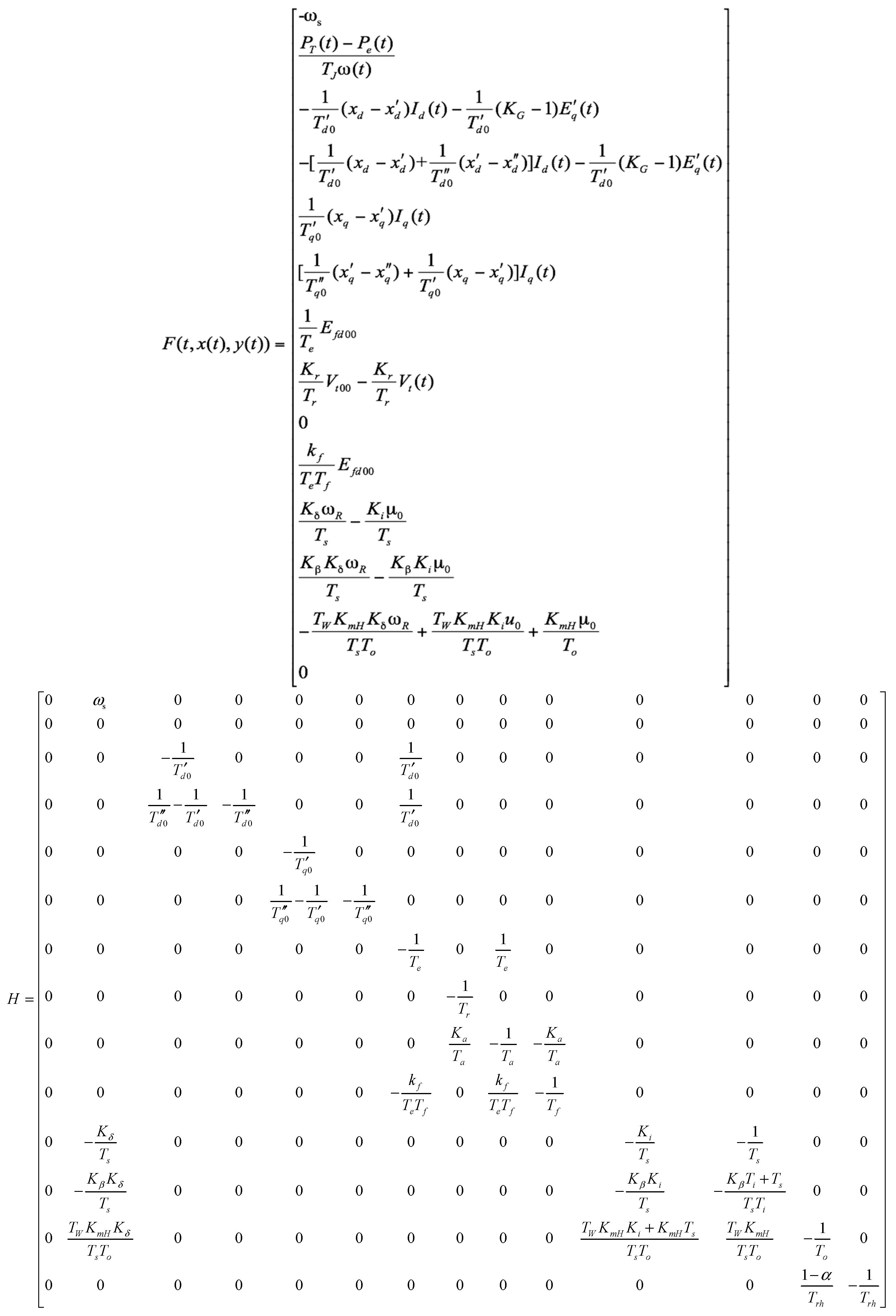
Figure 4.
Simulation results for the power angle using different integration algorithms. (a) power angle curves using different integration algorithms for case A; (b) power angle curves using different integration algorithms for case B; (c) power angle curves using different integration algorithms for case C; (d) partial enlargement of (a); (e) partial enlargement of (b); (f) partial enlargement of (c).
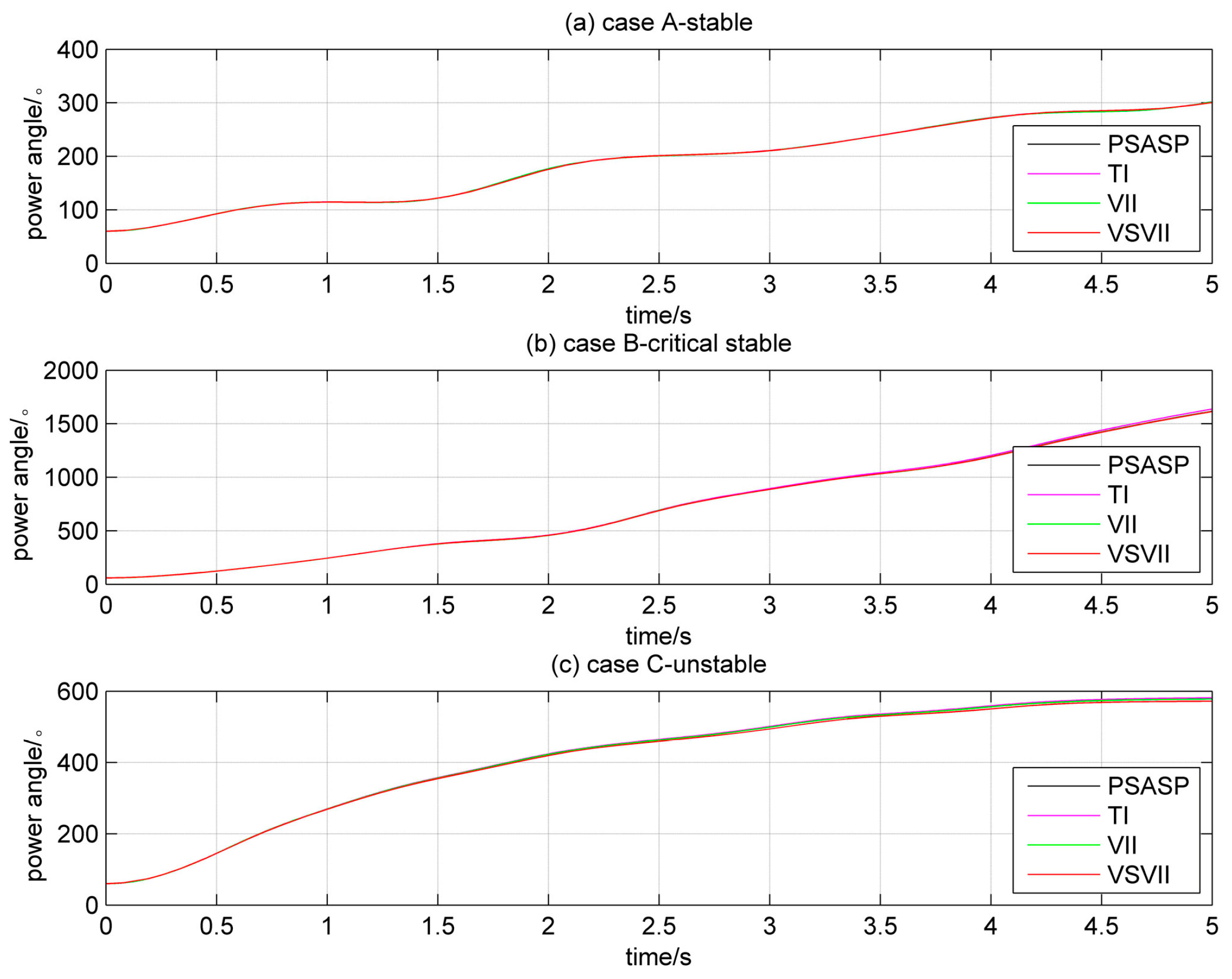

Figure 5.
Power angle using different step sizes in case A.

Figure 6.
Power angle using different step sizes in case B.

Figure 7.
Power angle using different step sizes in case C.
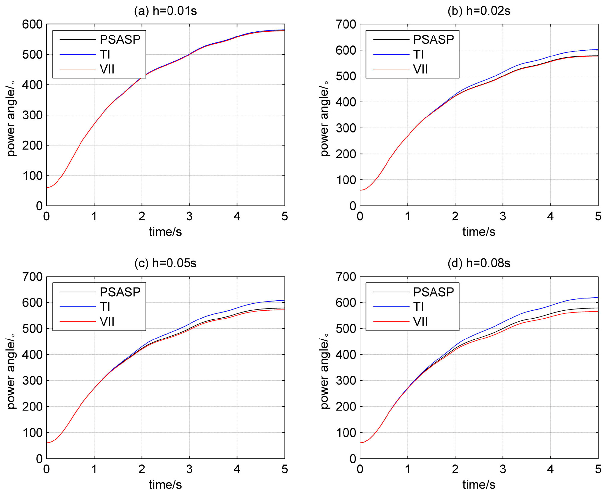
Figure 8.
The amount of computing for differential algebraic equations in case A.

Figure 9.
The amount of computing for differential algebraic equations in case B.

Figure 10.
The amount of computing for differential algebraic equations in case C.
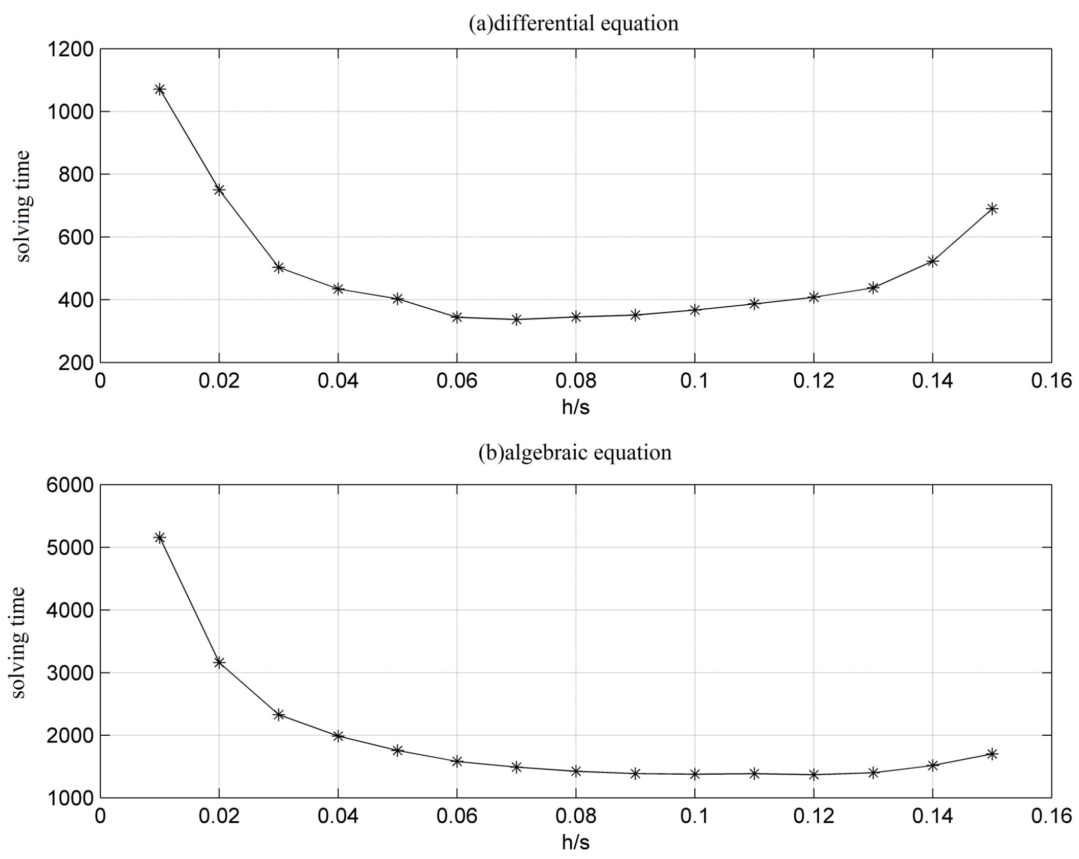
Figure 11.
The variation in the step size and iteration times using VSVII in case A.

Figure 12.
The variation in the step size and iteration times using VSVII in case B.
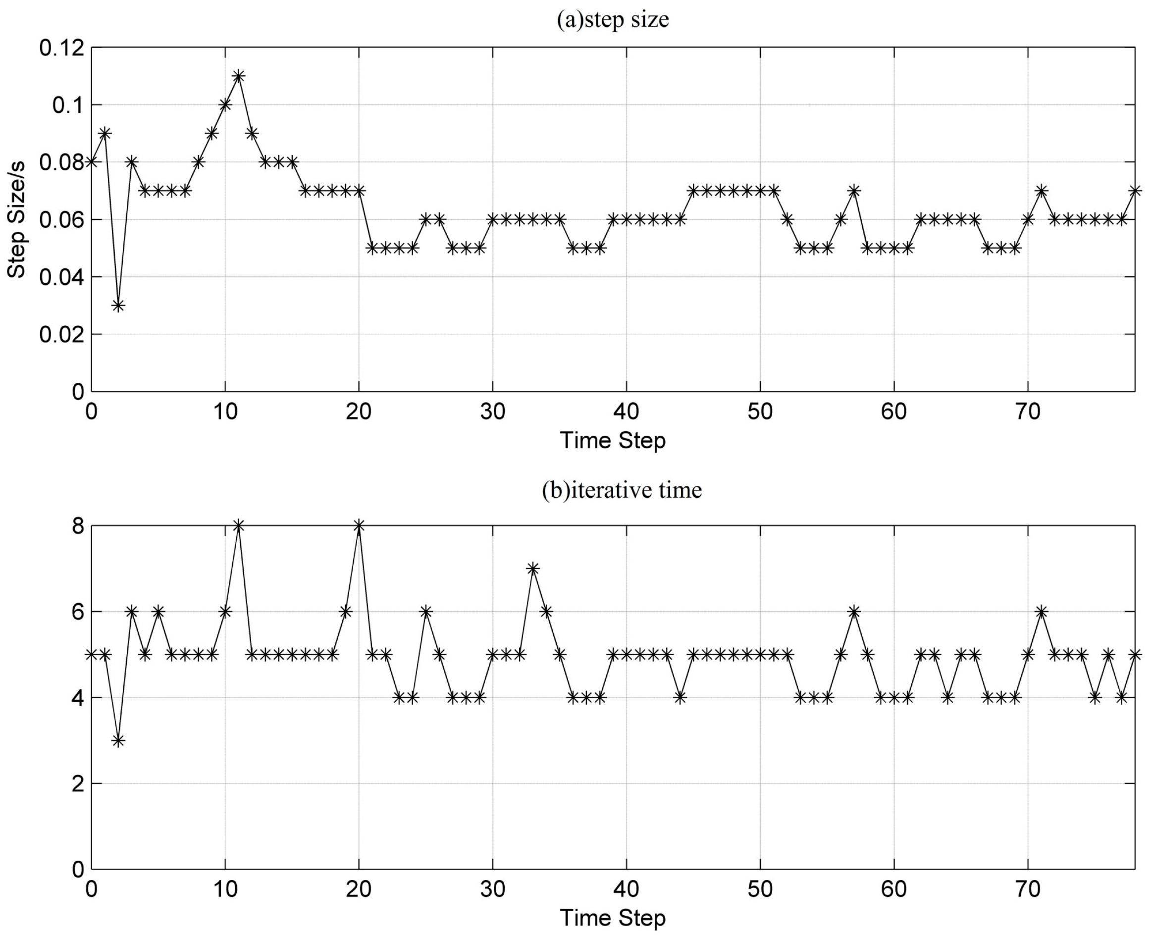
Figure 13.
The variation in the step size and iteration times using VSVII in case C.

Table 1.
Simulation results for the IEEE39 system.
| Simulation Results for Case A | ||||||
| Step Size (s) | Algorithm | Repetitions to Solve the Differential Equations | Repetitions to Solve the Algebraic Equations | The Number of Time Steps | Maximum Power Angle Difference (Degrees) | Computing Time (ms) |
| 0.01 | TI | 1073 | 4441 | 500 | 91.19 | 35.94 |
| VII | 1000 | 4361 | 91.15 | 32.41 | ||
| 0.02 | TI | 750 | 2785 | 250 | 90.90 | 29.63 |
| VII | 750 | 2765 | 91.14 | 28.33 | ||
| 0.05 | TI | 636 | 1886 | 100 | 90.53 | 25.21 |
| VII | 394 | 1458 | 91.13 | 16.76 | ||
| 0.08 | TI | 1178 | 2427 | 63 | 90.42 | 27.71 |
| VII | 359 | 1212 | 90.97 | 12.68 | ||
| VSVII | 380 | 1219 | 60 | 90.57 | 17.27 | |
| Simulation Results for Case B | ||||||
| Step Size (s) | Algorithm | Repetitions to Solve the Differential Equations | Repetitions to Solve the Algebraic Equations | The Number of Time Steps | Maximum Power Angle Difference (Degrees) | Computing Time (ms) |
| 0.01 | TI | 1415 | 6725 | 500 | 174.70 | 58.80 |
| VII | 1307 | 6465 | 174.36 | 41.18 | ||
| 0.02 | TI | 859 | 4214 | 250 | 172.40 | 30.97 |
| VII | 750 | 3752 | 174.41 | 29.40 | ||
| 0.05 | TI | 728 | 2855 | 100 | 170.58 | 33.87 |
| VII | 412 | 2153 | 174.72 | 16.62 | ||
| 0.08 | TI | 1333 | 3527 | 63 | 172.07 | 38.63 |
| VII | 376 | 1804 | 175.41 | 18.95 | ||
| VSVII | 388 | 1936 | 79 | 174.96 | 22.44 | |
| Simulation Results for Case C | ||||||
| Step Size (s) | Algorithm | Repetitions to Solve the Differential Equations | Repetitions to Solve the Algebraic Equations | The Number of Time Steps | Maximum Power Angle Difference (Degrees) | Computing Time (ms) |
| 0.01 | TI | 1176 | 5283 | 500 | 338.19 | 46.17 |
| VII | 1071 | 5157 | 336.64 | 31.83 | ||
| 0.02 | TI | 750 | 3374 | 250 | 344.93 | 40.67 |
| VII | 750 | 3162 | 335.90 | 23.99 | ||
| 0.05 | TI | 652 | 2312 | 100 | 346.43 | 26.53 |
| VII | 403 | 1756 | 333.91 | 16.52 | ||
| 0.08 | TI | 1228 | 2902 | 63 | 351.32 | 32.34 |
| VII | 345 | 1424 | 331.11 | 16.83 | ||
| VSVII | 390 | 1740 | 98 | 333.68 | 18.80 | |
Table 2.
Simulation results for a regional power system in China.
| Case Type | Algorithm | Repetitions to Solve the Differential Equations | Repetitions to Solve the Algebraic Equations | The Number of Time Steps | Maximum Power Angle Difference (Degrees) | Computing Time (s) |
|---|---|---|---|---|---|---|
| Stable | TI | 1014 | 1674 | 500 | 93.34 | 1.40 |
| VSVII | 907 | 1498 | 490 | 93.38 | 1.17 | |
| Critical Stable | TI | 1035 | 1912 | 500 | 178.48 | 1.36 |
| VSVII | 1010 | 1703 | 495 | 185.78 | 1.18 | |
| Unstable | TI | 1816 | 3454 | 500 | 413.52 | 1.96 |
| VSVII | 1307 | 2370 | 497 | 408.18 | 1.51 |
© 2017 by the authors. Licensee MDPI, Basel, Switzerland. This article is an open access article distributed under the terms and conditions of the Creative Commons Attribution (CC BY) license (http://creativecommons.org/licenses/by/4.0/).
Share and Cite
MDPI and ACS Style
Gao, Y.; Wang, J.; Xiao, T.; Jiang, D. A Transient Stability Numerical Integration Algorithm for Variable Step Sizes Based on Virtual Input. Energies 2017, 10, 1736. https://doi.org/10.3390/en10111736
AMA Style
Gao Y, Wang J, Xiao T, Jiang D. A Transient Stability Numerical Integration Algorithm for Variable Step Sizes Based on Virtual Input. Energies. 2017; 10(11):1736. https://doi.org/10.3390/en10111736
Chicago/Turabian StyleGao, Yifan, Jianquan Wang, Tannan Xiao, and Daozhuo Jiang. 2017. "A Transient Stability Numerical Integration Algorithm for Variable Step Sizes Based on Virtual Input" Energies 10, no. 11: 1736. https://doi.org/10.3390/en10111736
Note that from the first issue of 2016, this journal uses article numbers instead of page numbers. See further details here.