A Human-Machine-Cooperative-Driving Controller Based on AFS and DYC for Vehicle Dynamic Stability


1
School of Mechanical and Automotive Engineering, Liaocheng University, Liaocheng 252000, China
2
State Key Laboratory of Automotive Safety and Energy, Tsinghua University, Beijing 100084, China
*
Author to whom correspondence should be addressed.
Energies 2017, 10(11), 1737; https://doi.org/10.3390/en10111737
Submission received: 20 September 2017
/
Revised: 12 October 2017
/
Accepted: 24 October 2017
/
Published: 30 October 2017
(This article belongs to the Special Issue The International Symposium on Electric Vehicles (ISEV2017))
Abstract
:It is a difficult and important project to coordinate active front steering (AFS) and direct yaw moment control (DYC), which has great potential to improve vehicle dynamic stability. Moreover, the balance between driver’s operation and advanced technologies’ intervention is a critical problem. This paper proposes a human-machine-cooperative-driving controller (HMCDC) with a hierarchical structure for vehicle dynamic stability and it consists of a supervisor, an upper coordination layer, and two lower layers (AFS and DYC). The range of AFS additional angle is constrained, with consideration of the influence of AFS on drivers’ feeling. First, in the supervisor, a nonlinear vehicle model was utilized to predict vehicle states, and the reference yaw rate, and side slip angle values were calculated. Then, the upper coordination layer decides the control object and control mode. At last, DYC and AFS calculate brake pressures and the range of active steering angle, respectively. The proposed HMCDC is evaluated by co-simulation of CarSim and MATLAB. Results show that the proposed controller could improve vehicle dynamic stability effectively for the premise of ensuring the driver’s intention.
1. Introduction
Automobile safety issues have been a concern for a long time. Vehicle dynamics control (VDC) is a key technology of vehicle active safety and has already made much progress [1,2,3,4,5]. Direct yaw moment control (DYC) can control vehicle motion by an additional yaw moment generated with intentional distribution of tire longitudinal forces [6]. Thus, it can improve the vehicle stability and safety. VAN Zanten AT of Bosch company first proposed the combination of active yaw moment control (AYC) and slip ratio control, and developed a product to improve the vehicle stability [1]. Also, many researchers have studied VDC and vehicle-state observation in the past two decades [2,7,8,9,10].
With the development of intelligent vehicle technologies, many advanced technologies such as active braking, active suspension system (ASS), and active front steering (AFS) are applied to VDC [11,12,13,14]. ASS can isolate the vibration of vehicle body and keep the rider comfortable through reducing the sprung mass acceleration and providing adequate suspension deflection [15,16]. AFS can add an extra angle to the driver’s steering angle, utilizing the front steering command to improve vehicle lateral stability [17,18]. All of the above subsystems of the vehicle chassis can improve the performance of vehicles. However, the interaction and coordination of subsystems and structure of chassis systems must be well organized to facilitate the functionality of each subsystem and to achieve maximum performance [14].
The coupling among individual subsystems and diversity of their control strategies are two difficulties in coordinating subsystems [14,19,20]. Many have studied the coordination of those subsystems recently. J. Yoon et al. proposed a unified chassis control strategy to prevent vehicle rollover, and improve vehicle lateral stability by integrating electronic stability control and continuous damping control [19]. The combination of DYC and AFS is studied in references [21,22,23,24], considering the generation of corrective yaw moment to improve vehicle handling stability. Meanwhile, many related issues such as the uncertainty of tire cornering stiffness, onboard network-induced time delays, and control strategies were concerned gradually with the coordination of subsystems [21,25]. Selby et al. investigated the principle of the coordination of AFS and DYC, and proposed a coordination controller [11]. Falcone et al. utilized a model predictive control (MPC) approach in AFS to track a desired path for obstacle avoidance [12,26,27]. Yang et al. designed a coordination scheme based on optimal guaranteed cost control [21]. An adaptive integrated control algorithm based on AFS and DYC using the direct Lyapunov method was proposed by [28]. A gain scheduled linear parameter varying controller synthesized within the linear matrix inequalities was designed to coordinate AFS and DYC in [29]. The influence of the variation of longitudinal velocities and lateral accelerations was investigated in [13,30]. Shuai et al. designed a combined AFS and DYC controller with good robustness against in-vehicle-network induced time-varying delays [25]. With in-depth study of the coordination of AFS and DYC, more subsystems’ coordination has gradually attracted much interest [14]. Zhao et al. proposed an integrated controller to coordinate the interactions among ASS, AFS and DYC [14]. However, the construction of ASS requires higher production costs than other suspension systems, and the car model is practically denoted as a complicated system, so the derivation of active control technologies becomes relatively complicated [15]. Considering the implementation of actual chassis controls and the high cost of ASS, this paper researches the coordination of AFS and DYC, based on existing research results.
With the development of automotive automation, the balance between the driver’s operation and advanced technologies’ intervention, becomes a critical problem, especially for AFS, which directly influences the driver’s steering feel [31,32]. Navarro et al. carried out experiments and analyzed drivers’ steering behaviors and eye movement when AFS was used to steer a vehicle [33]. Minaki et al. designed a controller based on driver sensitivity characteristics to control the reactive torque and it is able to reduce the interference to a driver during the AFS operation [31]. In [32], Minaki et al. proposed a method of reducing steering interference and controlling the torque transmitted to the driver, by means of differential mechanical steering and utilizing planetary gears. J. Yoon et al. presented the range of AFS with respect to the tire slip angle in [20]. However, most of the existing studies of the coordination of AFS and DYC have not considered the driver’s steering feel when AFS operates, and the realization of the steering mechanism. Some coordination controllers may calculate a huge, even unrealizable, active front steering angle, which may be contrary to the driver’s intention and cause drivers emotional tension. Thus, the driver’s acceptability of active steering angles must be concerned.
Model predictive control (MPC) is robust and has been used widely in intelligent vehicle control. It can predict many vehicle dynamics states, and optimize multiple control objectives under many constraints [4]. A control scheme using the model predictive control method with the correction of clutch wear based on the estimation of resistance, was proposed in [34]. A three-dimensional dynamic stability controller was designed for yaw-roll stability control [4]. Falcone et al. utilized MPC in AFS to track a desired path for obstacle avoidance [12,27,28].
Considering the advantages of MPC, and the balance between driver operation and advanced technologies’ intervention, a human-machine-cooperative-driving controller (HMCDC) with a hierarchical structure was designed, based on MPC to coordinate AFS and DYC. The range of the active steering angle is presented explicitly. To verify the effectiveness of our proposed controller, we treated control and models properly [35,36,37,38]; for example, X. Hu et al. proposed a model-based dynamic power assessment, and designed controllers and models properly to verify their work [38]. The HMCDC is evaluated by co-simulation of CarSim (8.02) and MATLAB (R2014a). CarSim gives the full-vehicle model and the proposed controller is developed with MATLAB Simulink. This paper is organized as follows: in Section 2, the nonlinear vehicle dynamics model is presented. Section 3 gives a description about the controller. Then its performance is evaluated by co-simulation of CarSim and MATLAB in Section 4. Finally, the conclusion is presented in Section 5.
2. Related Models
2.1. Vehicle Dynamics Model
A simplified four wheel vehicle dynamics model is demonstrated in Figure 1. The longitudinal, lateral and yaw motion can be described as follows:
The rotation equations of four wheels are as follows:
where and are the longitudinal and lateral forces of four wheels, their subscript ij is fl, fr, rl, and rr, representing the front left, front right, rear left and rear right wheel respectively, ij used in the following equations has the same meaning. m is the mass of vehicles, JW is the wheel inertia moment about the rotary axis, and Iz is the inertia moment about the vertical axis of vehicles. Vx and Vy are the longitudinal and lateral velocities respectively, β represents the side slip angle, and ωr represents the yaw rate. δ is the steering angle. a and b are the distance from the gravity center to the front and rear axles respectively, and T is the distance between the left and right wheel. R is the wheel radius. ωij is the wheel angular speed. Ttij and Tbij represent the driving torques and braking torques respectively.
The position of a vehicle in the vehicle axis system should be transformed into the absolute inertial frame. The following equations represent vehicle motions in absolute inertial frame:
where and are the vehicle longitudinal and lateral velocities in the absolute inertial frame respectively.
2.2. Nominal Values Calculation Model
A 2-degree of freedom (DOF) bicycle model is utilized to calculate the nominal values of yaw rate and side-slip angle, which are selected as the reference values. The nominal values can be described as follows:
where is the steady-state yaw rate, δ is the front wheel angle, l is the wheel base, βs is the side-slip angle nominal value, and K is the stability factor, which can be calculated as follows:
where k1 and k2 are the cornering stiffness of front and rear axles respectively.
2.3. Tire Model
The tires are usually at the non-linear regions when VDC begins to work. Pacejka’s magic formula (MF) is used to describe the tires’ dynamics. The longitudinal and lateral tire forces can be calculated by MF. Its general form can be described as follows:
where Y(x) can represent longitudinal tire forces Fx, lateral tire forces Fy, and aling torques Mz and x can be the longitudinal slip ratio λ, and the wheel side-slip angle α.
The longitudinal slip ratio can be calculated as follows:
where Vxij represents the longitudinal velocities of four wheels, ωij is angular velocities of four wheels, and Vωij are their linear velocities respectively.
The side-slip angle α can be calculated as follows:
where αfj represents the side-slip angles of front wheels and αrj represents the side-slip angles of rear wheels.
The parameters in the MF can be calculated as in [4].
3. Design of HMCDC
The diagram of the proposed controller is demonstrated in Figure 2. It consists of a supervisor, an upper coordination layer, and two lower layers (AFS and DYC). In the supervisor, considering the constraints of tire-road adhesion, the nonlinear vehicle dynamics model with MF tire model is utilized to predict vehicle states. Moreover, the reference yaw rate and side-slip angle can be calculated. The coordination control strategy, designed with the premise of guaranteeing the driver’s intention and minimizing the influence on the driver’s steering feel and the active steering angle range, is discussed explicitly. To the best of our knowledge, the range of AFS additional steering angle is defined for the first time. The control modes consist of AFS mode, and hybrid mode. The lower layers are designed to realize the corrected angle and the additional yaw moment.
3.1. The Supervisor
The reference values are essential parameters of MPC, and we used the nominal values of yaw rate and side-slip angle calculated by the 2 DOF bicycle model as the reference values. They can be calculated by the Equations (7) and (8). Due to constraints of tire-road adhesion coefficient μ, the upper limit of yaw rate can be described as follows:
The side-slip angle also needs to be modified, considering the tire-road adhesion:
We also take into consideration the transient characteristics of actual vehicle operation, and a first-order filter is utilized to modify the nominal values as follows:
where τω and τβ are the inertia constants.
The proposed controller needs many vehicle states, and a nonlinear vehicle model is utilized to predict vehicle future states, based on the current states and vehicle inputs. The equipped sensors in vehicles can directly measure ωr, ay, δ, and some other parameters such as tire forces, vehicle longitudinal and lateral velocities, and the road-tire friction coefficient can be obtained through observers and estimators. The driving torques Ttij can be measured by the engine management system and the braking torques Tb can be calculated through braking pressures Pb as follows [39]:
where η is the braking efficiency, Re is the brake plate equivalent radius, μp represents the brake pad friction coefficient, and Ap is the wheel cylinder cross-sectional area.
To coordinate AFS and DYC properly based on the vehicle states, a coordination factor is denoted by CF as follows:
where ay, β are the lateral acceleration and side slip angle, and a, b denote their weights respectively.
The prediction of vehicle states utilizes the model in Section 2, and a quadratic polynomial extrapolation method is utilized to predict the driver’s steering input [3]. The nonlinear model in Section 2 is discretized with the Euler method:
where Vx(n), β(n) and ωr(n) represent the longitudinal velocity, the side slip angle, and the yaw rate at time n respectively. ∆Vx(n), ∆β(n) and ∆ωr(n) can be calculated as follows:
The equations of wheel rotation are discretized as follows:
3.2. The Upper Layer
The upper layer can select its proper object: ensuring the yaw stability or the path-following capability, based on vehicle states. Then it decides the control mode: AFS control mode or hybrid AFS and DYC mode, and calculates the active steering angle range. When β is very large, hybrid AFS and DYC mode will work to ensure the yaw stability. When the vehicle is in the stability state, the upper layer’s object is to ensure the path-following capability and AFS mode works. It works alone near the linear tire characteristic region. In Figure 3, a two-dimension working region ay-β of control modes is defined and the proposed controller can determine which control mode to work, as Figure 3 describes. The selecting-control-mode strategy can be based on the defined coordination factor and side-slip angle. The working region of DYC and AFS can be defined on the basis of the wheel side-slip angle.
The algorithm flowchart is demonstrated as follows: when CF is smaller than CFth, the control object is to ensure that the path-following capability and AFS provide additional front wheel angles; when the vehicle is in the danger of loss of control, that is, when CF is larger than CFth, the control object is to ensure that the yaw stability and the control mode can be selected based on the tire side-slip characteristics. When β is smaller than βth, the hybrid AFS and DYC mode works. Otherwise, tires are in a strong nonlinear region, and AFS can provide an additional negative steering angle. The threshold CF value is set as follows:
Based on the side-slip characteristics, the threshold βth is set as follows:
The supervisor also calculates the predicted values CFpre and βpre. They are utilized as auxiliary conditions to decide the control object and mode.
On the premise of guaranteeing the driver’s intention and minimizing the influence on the driver’s steering feel, the range of the active steering angle is discussed explicitly. This is one of the main contributions from this research. The actual front wheel angle is different from the driver’s input, due to the additional active steering angle. Based on the acceptability of active steering angles we set the limit curves of the AFS operating range:
where δAFS is the additional active steering angle and represents the set of the additional AFS angle.
Then the AFS control range can be obtained through the upper and lower limit calculated by Equations (68) and (69). In the designed control range, the additional active steering angle has a relatively small effect on the driver’s steering feel. Maintaining the driver’s operation intention areas means that the controller should control l the proportion of vehicle’s response to the driver’s operation. Additionally, considering the realization of the steering mechanism, the control input should be limited by δth which we define as follows:
Considering the longitudinal motion, the lateral motion, the yaw motion, and the vehicular motion in the absolute inertial frame, we define the state variables as follows:
The control inputs of the upper layer are the tire forces of the four wheels and the front wheel steering angle:
The state space model of the designed HMCDC can be described as follows:
where
Then, Equation (35) is discretized by Taylor expansion and discretization. It can be reconstructed into the standard discrete and incremental form as follows:
where
∆T is the sample time.
We define that the controlled outputs of the upper layer are the side-slip angle, the yaw rate and the lateral position as follows:
where:
Considering the realization of the steering mechanism and the ability of the brake system, we set the range of control input as follows:
where δth is defined as the Equation (49). ∆δmin and ∆δmax are the minimum and maximum increments of the front wheel angles and their values are dependent on the steering system. ∆umin and ∆umax are the minimum and maximum increments of four wheels. We set their values based on the maximum release rate and the maximum increase rate of brake system. Fxij-min represents the minimum tire forces of four wheels. Previous researches calculated their values by the adhesion ellipse. However, the brake intervention of DYC may produce an unpleasant feeling for the driver due to the coordination of AFS and DYC, so we set the modified calculation of Fxij-min to minimize the unpleasant feeling caused by DYC as follows:
where we define that γAFS is the AFS constriction factor and ρ is a coefficient smaller than one.
The designed HMCD based on MPC should ensure that the controlled outputs track the reference values precisely, and the control inputs are as small as possible at the same time. Therefore we define that the MPC objective function is as follows:
where yc is the controlled output and yref is the reference output. Np is the prediction horizon, Nc is the control horizon, and Np ≥ Nc. Qi and Ri are the weight matrices of the controlled outputs and the control inputs at the prediction time k + i respectively. The standard forms of Qi and Ri are as follows:
where Wβ, Wωr, WY, Wδ, and WFxij are weight factors of β, ωr, Y, δ, Fxij respectively.
The upper layer should minimize the objective function (69) subject to the control input constraints (66), (67), and the vehicle dynamics (62). We can define the equations as follows:
Subject to:
Equations (54) and (55) present a typical mathematical optimal problem and the function quadprog of MATLAB is utilized to calculate the optimal solution. Moreover, the problem can be solved under constrains and the optimal outputs can be calculated. As long as the objective function can be solved, the minimums must be achieved.
The upper layer has two control objects, and its design is mainly based on the yaw rate error, the side-slip angle error, and the lateral position error. Therefore a different matrix, Qi is designed for the corresponding control object. We define the weights of the controlled outputs for ensuring the yaw stability of vehicles as follows:
For the path-following object, the designed layer provides an additional active steering angle to improve the path following capability. The weights can then be set as follows:
The weights of controlled inputs should be different for different control modes. DYC can control the longitudinal tire forces, and AFS provides additional front wheel angle. Therefore, the weights for the AFS mode are:
When the control mode is the DYC and AFS mode, both the brake system and the steering system work to ensure the stability of the vehicle. We define the weights as follows:
The value of κ should increase with the decrease of the wheel side-slip angle, or the CF value. κ is designed as follows:
where ς can be calculated as follows:
3.3. The Lower Layer
The lower DYC layer can realize the calculated tire forces from the upper layer. We can calculate the desired slip ratio, which is smaller than the optimum slip ratio λopt based on the tire forces from the upper layer. The desired slip ratio λdes can be obtained by the dichotomy method in [40]. The desired pressure Pdes can be calculated as follows [41]:
where Ap is the piston area, Rb is the effective radius between the center of disk rotor and pad, and is the estimated brake disk-pad friction coefficient. Jw is the moment of inertia of wheel, rw is the radius of the wheel, λ is the wheel slip ratio, and s is the sliding surface. What is more, the bound values of the uncertainties B1, B2, and B3 are 0.6, 1500, 0.35 respectively. η is a design parameter and a strictly positive constant, Φ is a design parameter representing the boundary layer around the s = 0 sliding surface, and is a small positive parameter. A first-order filter is utilized to realize the real characteristics of brake systems as follows:
where Preal is the real brake pressure input of CarSim and τp is the time coefficient, where we define its value as 0.2 in this paper.
The desired front wheel angle is calculated by the upper layer. The lower AFS layer is designed to realize the additional active steering angle, based on the desired front angle and the driver’s input. We can calculate the additional active steering angle as follows:
Subject to:
A first-order filter is utilized to realize the real characteristics of steering systems as follows:
where τAFS is the time coefficient, which we define as a value of 0.01 in this paper.
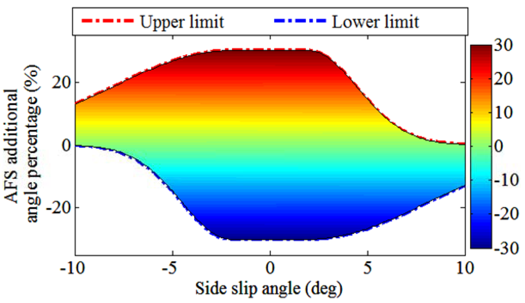
We define the upper and lower limits of the AFS angle based on the tire characteristics, and the AFS angle range can be defined by the value of side slip angle as shown in Figure 4. The percentage of the AFS additional angle changes with the side slip angle. We define the upper and lower limit as follows:
where δAFS-upper and δAFS-lower denote the AFS additional angle range limits. We define that κ is the peak factor, σ is the buckling factor, ρ is the curvature correction factor, and ε is the turning factor.
As shown in Figure 4, when the side-slip angle is small, which means tires work in a linear region, the AFS additional angle percentage can be large in both a positive and negative direction. If the side-slip angle is extremely large, which means tires are at a highly nonlinear state, the additional angle in a positive direction will not work, or even worsen vehicle dynamics states, while a small negative additional angle may improve vehicle dynamics stability. Therefore, the additional angle in a positive direction tends to zero, and in negative direction, it becomes smaller with the increase of side-slip angle.
4. Simulation Results and Analysis
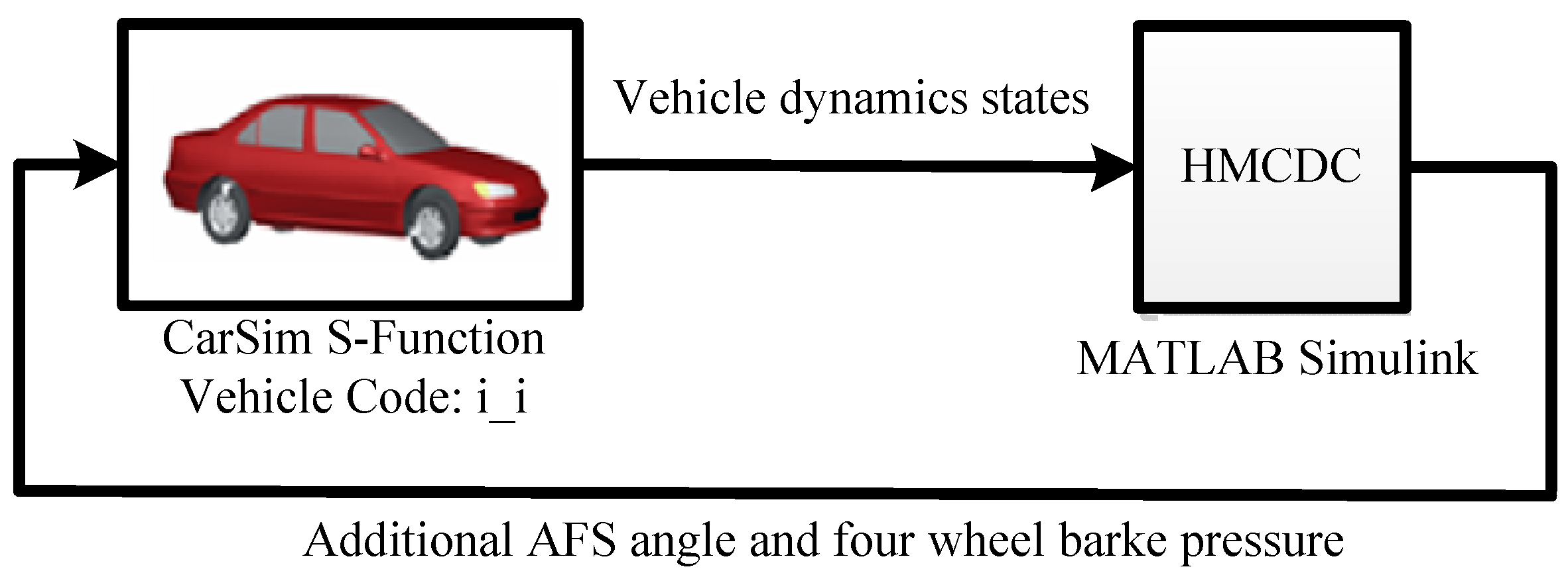
The HMCDC was evaluated by co-simulation of CarSim and MATLAB as shown in Figure 5. CarSim is a professional commercial simulation software for vehicle dynamics, and it can provide a MATLAB Simulink interface to run in Simulink. CarSim provides a the full-vehicle model, and the proposed controller is developed with MATLAB Simulink as shown in Figure 5. Then, critical scenarios can be implemented to verify and evaluate performance. When a car runs at a high speed on the highways, emergency avoidance at a high speed may cause vehicle dynamics instability. Therefore, we imitated a critical scenario above utilizing a double lane change (DLC) maneuver with an initial speed 115 km/h, to verify the effectiveness of our proposed controller. Based on the actual highway situation, we set that the maximum lateral offset of DLC maneuver would be 3.59 m and the friction coefficient μ was 0.80. The driver model utilized in CarSim had a constant preview time of 0.7 s. We also utilized a conventional electronic stability control (ESC) controller which only used DYC. The DYC was also based on the same model and MPC as the proposed controller.
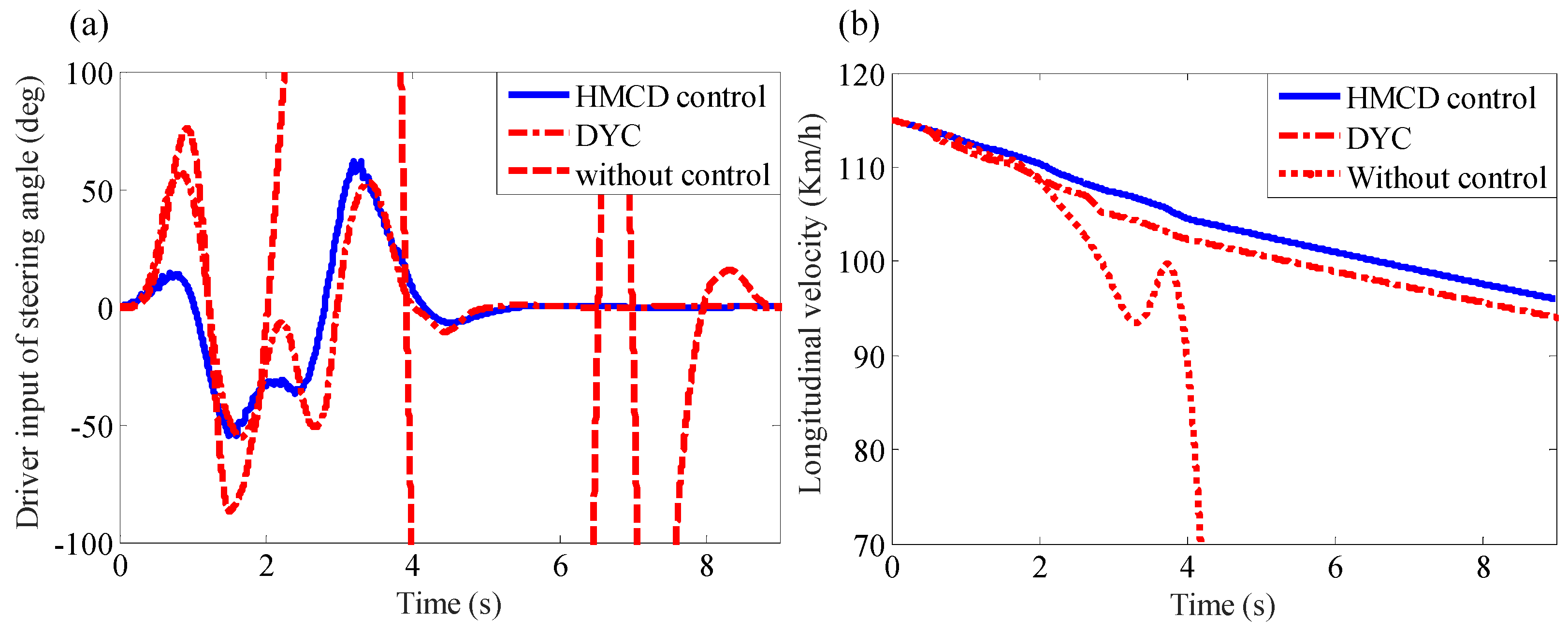
The steering wheel angles of the preview driver model (PDM) with different controllers are compared in Figure 6. The PDM utilized in CarSim can imitate a driver controlling a steering wheel. The steering wheel angle, without any stability control reached extremely large values and changed sharply, which means that the vehicle motion was out of control. However, PDM gave suitable steering wheel angles to keep vehicle dynamics stability with the assistance of the HMCDC or conventional ESC. We also found that most of the steering wheel angle with the proposed HMCDC was smaller than the angle reached with conventional ESC, due to AFS. The steering wheel angle with the stability control reached zero at about 5.9 s, but without any control, the PDM gave zero steering wheel angle at about 9 s. Also, as shown in Figure 6, the longitudinal velocity without any control fell sharply, but fell slowly and smoothly with HMCDC or DYC. The longitudinal velocity controlled by the HMCDC was larger than that controlled by the conventional ESC because the HMCDC needed less brake intervention than DYC to keep vehicle dynamics stable.
The nominal value was calculated through the ideal response of a 2 DOF vehicle model. The error between the nominal value and the actual value indicated vehicle dynamics stability state. When the error between the actual value of yaw rate or side-slip angle and its nominal value was small, the vehicle runs at dynamics stability state. On the contrary, a large error meant that the vehicle was out of control, and lost its dynamics stability. When the car ran without control, the actual side-slip angle and yaw rate was divergent, as shown in Figure 7 and Figure 8, which meant that the car swerved severely and was out of dynamics stability. With our proposed controller, the actual value was almost equal to the corresponding nominal value, which indicated that the car was at a dynamics stability state, as shown in Figure 7 and Figure 8.
The results illustrate that the proposed HMCDC can perform better with less brake intervention than the conventional ESC, due to the regulating action of AFS as shown in Figure 7. The actual side slip angle controlled by the proposed HMCDC can track the nominal value more accurately than that controlled by DYC. We found that the maximum error value controlled by the HMCDC was 0.63° at 0.79 s, while the value controlled by DYC was 2.41° at 2.26 s. In Figure 6, we also found that the maximum side slip angle value controlled by the HMCDC was 2.1° at 2.73 s, smaller than that controlled by DYC, which was 3.90° at 2.19 s. This means that the HMCDC can control the vehicle more stably than DYC. In Figure 8, the nominal and actual yaw rate value is shown, and we found that with HMCDC or DYC, the yaw rate changed smoothly, but it changed sharply without any control.
As shown in Figure 9b the lateral acceleration with the proposed HMCDC was similar to that with DYC, but the maximum value with DYC was 0.73 g, approximately 2 s larger than the lateral acceleration with the HMCDC control, which was 0.637 g at about 2.6 s. In Figure 9a, the trajectories with different controllers was shown and we found that the trajectory controlled by the HMCDC tracked more precisely than that controlled by DYC. The maximum Y error value with a proposed controller was smaller than that with DYC, as shown in Figure 9a.
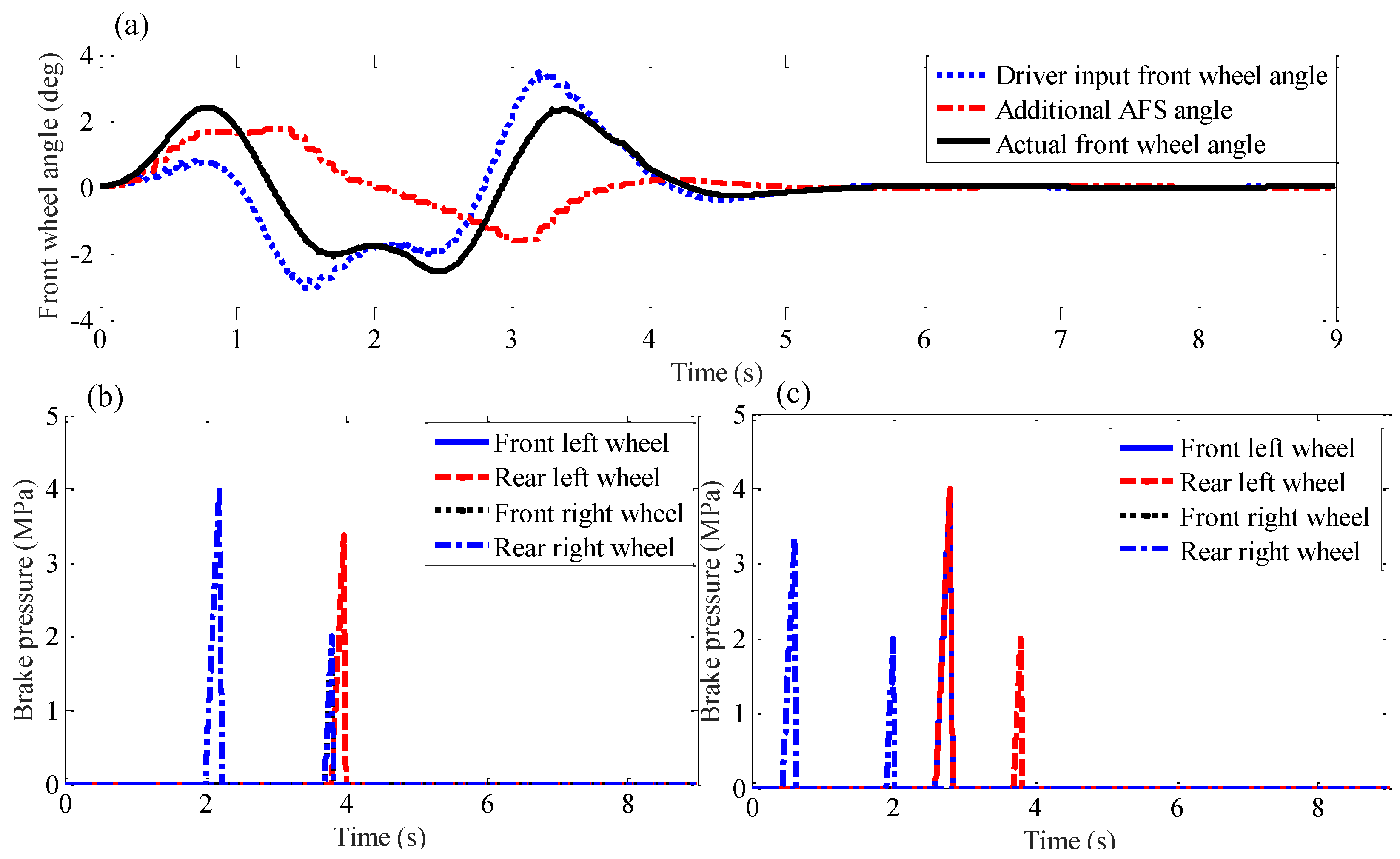
A Large brake force on the wheels can help to keep the vehicle stable, but influences the driver’s comfort negatively. The proposed controller could keep vehicular dynamics stability with less brake intervention, as shown in Figure 10. We found that the brake interventions controlled by DYC were approximately 3.9 MPa, 2.0 MPa, 4.1 MPa, and 2.0 MPa at 0.7 s, 2.0 s, 2.9 s, and 3.9 s respectively, while the brake interventions controlled by the proposed controller were about 4.0 MPa, and 3.7 MPa at 2.1 s, and 3.9 s respectively, due to the assistance of AFS, as shown in Figure 10b,c.
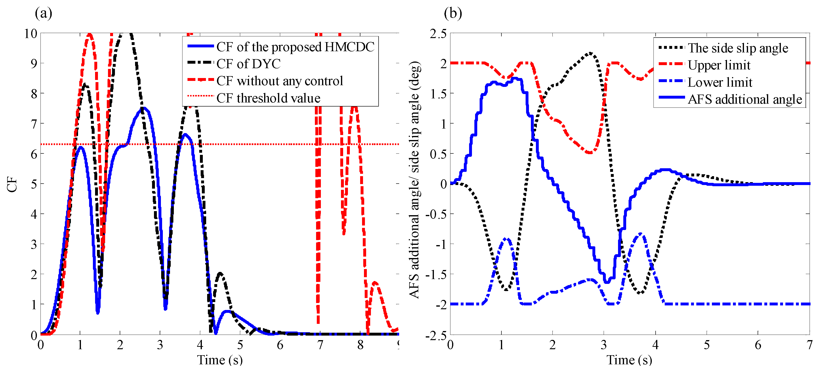
In Figure 10a, the additional AFS angle and the driver input front wheel angle are shown. we found that the maximum additional AFS angle was 1.74° at 1.3 s. The additional AFS angle increased the driver input on the front wheel angle from 0 s to 1 s, from 2 s to 2.5 s, and from 3.7 s to 4.2 s. The additional AFS angle decreased the driver input front wheel angle from 1 s to 2 s, and from 2.5 s to 3.7 s. As shown in Figure 11, the upper limit and lower limit of the additional AFS angle can be calculated based on the side slip angle. The limit value decreased when the side slip angle was very large, and the actual AFS angle controlled by the proposed HMCDC always adjusted within the limit, which means that the HMCDC can provide proper AFS additional angle on the premise of minimizing the influence on the driver’s steering feel.
In Figure 11, the CF values indicating the dynamics stability state without any control fluctuated greatly, and most were beyond the CF threshold value defined in the proposed controller. However, the CF values with HMCDC or DYC possessed a similar trend and, only some of them were larger than the CF threshold value. The CF values controlled by HMCDC were mostly smaller than those controlled by DYC. We found that the maximum value controlled by HMCDC was 7.49 at 2.61 s, while the maximum value controlled by DYC was 10.20 at 2.16 s. The proposed HMCDC selects the AFS and DYC mode when the CF values are beyond the CF threshold respectively from 2.1 s to 2.9 s, and from 3.6 s to 3.9 s approximately. However, the CF values controlled by DYC were larger than the threshold value respectively, from 0.8 s to 1.3 s, from 1.8 s to 2.7 s, and from 3.4 s to 4.1 s. The results shown in Figure 11 indicate that the proposed HMCDC performs better than DYC on vehicle dynamics stability control.
5. Conclusions
This paper proposes a HMCDC to coordinate DYC and AFS, considering the driver’s acceptability of active steering angles. It consists of a supervisor, an upper coordination layer, and two lower layer (AFS and DYC). The main contributions of this paper can be summarized as follows. A HMCDC with a hierarchical structure is designed, based on MPC to coordinate AFS and DYC. Moreover, a two-dimension working region ay-β of AFS and DYC is defined based on vehicle body side-slip angle and lateral acceleration. Furthermore, the upper and lower limits of the additional AFS angle are designed based on tire characteristics, and the relationship between AFS additional angle percentage and side-slip angle is defined explicitly.
The co-simulation results showed that the designed controller can improve the path-following capability and vehicle lateral stability. The coordination between DYC and AFS performs well, and AFS performed on the premise of guaranteeing the driver’s intention and minimizing the influence on the driver’s steering feel. The AFS angle range was defined, but the limit may still need to be modified by large-scale data analysis of different drivers’ actual runs, and this may form the basis for future work. Moreover, the simulation of low friction surfaces and hardware-in-the-loop simulations, or even real car tests, may be conducted in the future. The time-delay and bandwidth of actuators are important issues of real-car applications for our proposed controller. In future work, they will be studied to apply our proposed controller to a real vehicle.
Acknowledgments
This project was supported by Natural Science Foundation of Shandong Province (ZR2016EEQ06), the National Science Fund of the Peoples Republic of China (Grant No. 51675293), and The National Key Research and Development Program of China (Grant No. 2016YFB010140X).
Author Contributions
Shuo Cheng conceived and designed the experiments; Binhao Liu and Shuo Cheng performed the experiments; Jian Wu and Shuo Cheng analyzed the data; Shuo Cheng and Congzhi Liu contributed reagents/materials/analysis tools; Jian Wu wrote the paper.
Conflicts of Interest
The authors declare no conflict of interest.
References
- Li, L.; Wang, X.; Song, J. Fuel consumption optimization for smart hybrid electric vehicle during a car-following process. Mech. Syst. Signal Process. 2017, 87, 17–29. [Google Scholar] [CrossRef]
- Tsengh, E.; Ashrafi, B.; Madau, D.; Allen Brown, T.; Recker, D. The development of vehicle stability control at ford. IEEE/ASME Trans. Mechatron. 1999, 4, 223–234. [Google Scholar] [CrossRef]
- Zhu, H.; Li, L.; Jin, M.; Li, H.; Song, J. Real-time yaw rate prediction based on a non-linear model and feedback compensation for vehicle dynamics control. Proc. Inst. Mech. Eng. Part D J. Automob. Eng. 2013, 227, 1431–1445. [Google Scholar] [CrossRef]
- Li, L.; Lu, Y.; Wang, R.; Chen, J. A 3-Dimentional Dynamics Control Framework of Vehicle Lateral Stability and Rollover Prevention via Active Braking with MPC. IEEE Trans. Ind. Electron. 2016, 64, 3389–3401. [Google Scholar] [CrossRef]
- Goodarzi, A.; Naghibian, M.; Choodan, D.; Khajepour, A. Vehicle dynamics control by using a three-dimensional stabilizer pendulum system. Veh. Syst. Dyn. 2016, 54, 1671–1687. [Google Scholar] [CrossRef]
- Furukawa, Y.; Abe, M. Advanced Chassis Control Systems for Vehicle Handling and Active Safety. Veh. Syst. Dyn. 1997, 28, 59–86. [Google Scholar] [CrossRef]
- Zheng, S.; Tang, H.; Han, Z.; Zhang, Y. Controller design for vehicle stability enhancement. Control Eng. Pract. 2006, 14, 1413–1421. [Google Scholar] [CrossRef]
- Li, H. Reliability indexed sensor fusion and its application to vehicle velocity estimation. J. Dyn. Syst. Meas. Control 2006, 128, 236–243. [Google Scholar]
- Hsiao, T.; Tomizuka, M. Sensor fault detection in vehicle lateral control systems via switching kalman filtering. IEEE Trans. Control Syst. Technol. 2005, 15, 519–528. [Google Scholar]
- Xu, L.; Eric Tseng, H. Robust model-based fault detection for a roll stability control system. IEEE Trans. Control Syst. Technol. 2007, 15, 519–528. [Google Scholar] [CrossRef]
- Selby, W.; Manning, W.; Brown, M.; Crolla, D. A Coordination Approach for DYC and Active Front Steering; SAE Technical Paper Series; SAE 2001 World Congress: Detroit, MI, USA, 2001. [Google Scholar]
- Falcone, P.; Tseng, H.E.; Borrelli, F.; Asgari, J.; Hrovat, D. MPC-based yaw and lateral stabilisation via active front steering and braking. Veh. Syst. Dyn. 2008, 46, 611–628. [Google Scholar] [CrossRef]
- Zhang, H.; Wang, J. Vehicle lateral dynamics control through AFS/DYC and robust gain-scheduling approach. IEEE Trans. Veh. Technol. 2016, 65, 489–494. [Google Scholar] [CrossRef]
- Zhao, J.; Wong, P.K.; Ma, X.; Xie, Z. Chassis integrated control for active suspension, active front steering and direct yaw moment systems using hierarchical strategy. Veh. Syst. Dyn. 2016, 55, 72–103. [Google Scholar] [CrossRef]
- Yoshimura, T.; Kume, A.; Kurimoto, M.; Hino, J. Construction of an active suspension system of a quarter car model using the concept of sliding mode control. J. Sound Vib. 2001, 239, 187–199. [Google Scholar] [CrossRef]
- Kuo, Y.-P.; Li, S. GA-Based Fuzzy PI/PD Controller for Automotive Active Suspension System. IEEE Trans. Ind. Electron. 1999, 46, 1051–1056. [Google Scholar]
- Ackermann, J.; Bünte, T.; Odenthal, D. Advantages of Active Steering for Vehicle Dynamics Control. 1999. Available online: http://citeseerx.ist.psu.edu/viewdoc/download?doi=10.1.1.31.1688&rep=rep1&type=pdf (accessed on 30 October 2017).
- Falcone, P.; Borrelli, F.; Asgari, J.; Tseng, H.E.; Hrovat, D. Predictive Active Steering Control for Autonomous Vehicle Systems. IEEE Trans. Control Syst. Technol. 2007, 15, 566–580. [Google Scholar] [CrossRef]
- Yoon, J.; Cho, W.; Yi, B.K.K. Unified Chassis Control for Rollover Prevention and Lateral Stability. IEEE Trans. Veh. Technol. 2009, 58, 596–609. [Google Scholar] [CrossRef]
- Yoon, J.; Cho, W.; Yi, B.K.K. Unified Chassis Control for Rollover Prevention, Maneuverability and Lateral Stability. In Proceedings of the Advanced Vehicle Control, Kobe, Japan, 6–11 July 2008; pp. 708–713. [Google Scholar]
- Yang, X.; Wang, Z.; Peng, W. Coordinated control of AFS and DYC for vehicle handling and stability based on optimal guaranteed cost theory. Veh. Syst. Dyn. 2008, 47, 57–79. [Google Scholar] [CrossRef]
- Lee, B.; Khajepour, A.; Behdinan, K. Vehicle Stability through Integrated Active Steering and Differential Braking; SAE Technical Paper; SAE: Warrendale, PA, USA; Troy, MI, USA, 2006. [Google Scholar]
- Hamzah, N.; Aripin, M.K.; Sam, Y.M.; Selamat, H.; Ismail, M.F. Yaw stability improvement for four-wheel active steering vehicle using sliding mode control. In Proceedings of the 2012 IEEE 8th International Colloquium on Signal Processing and Its Applications (CSPA), Melaka, Malaysia, 23–25 March 2012; pp. 127–132. [Google Scholar]
- Di Cairano, S.; Tseng, H.E.; Bernardini, D.; Bemporad, A. Vehicle yaw stability control by coordinated active front steering and differential braking in the tire sideslip angles domain. IEEE Trans. Control Syst. Technol. 2013, 21, 1236–1248. [Google Scholar] [CrossRef]
- Shuai, Z.-B.; Shuai, H.; Wang, J.-M.; Li, J.-Q.; Ouyang, M.-G. Combined AFS and DYC Control of Four-Wheel-Independent-Drive Electric Vehicles over CAN Network with Time-Varying Delays. IEEE Trans. Veh. Technol. 2014, 63, 591–602. [Google Scholar]
- Falcone, P.; Borrelli, F.; Asgari, J.; Tseng, H.E.; Hrovat, D. A model predictive control approach for combined braking and steering in autonomous vehicles. In Proceedings of the Mediterranean Conference on Control & Automation (MED’07), Athens, Greece, 27–29 June 2007; pp. 1–6. [Google Scholar]
- Falcone, P.; Tufo, M.; Borrelli, F.; Asgari, J.; Tseng, H.E. A linear time varying model predictive control approach to the integrated vehicle dynamics control problem in autonomous systems. In Proceedings of the 2007 46th IEEE Conference on Decision and Control, New Orleans, LA, USA, 2–14 December 2007; pp. 2980–2985. [Google Scholar]
- Ding, N.; Taheri, S. An adaptive integrated algorithm for active front steering and direct yaw moment control based on direct Lyapunov method. Veh. Syst. Dyn. 2010, 48, 1193–1213. [Google Scholar] [CrossRef]
- Doumiati, M.; Sename, O.; Dugard, L.; Martinez-Molina, J.-J.; Gaspar, P.; Szabo, Z. Integrated vehicle dynamics control via coordination of active front steering and rear braking. Eur. J. Control 2013, 19, 121–143. [Google Scholar] [CrossRef] [Green Version]
- He, J.; Crolla, D.; Levesley, M.; Manning, W. Coordination of active steering, driveline, and braking for integrated vehicle dynamics control. Proc. Inst. Mech. Eng. Part D J. Automob. Eng. 2006, 220, 1401–1420. [Google Scholar] [CrossRef]
- Minaki, R.; Hoshino, H.; Hori, Y. Ergonomic verification of reactive torque control based on driver’s sensitivity characteristics for active front steering. In Proceedings of the IEEE Vehicle Power and Propulsion Conference (VPPC), Dearborn, MI, USA, 7–10 September 2009; pp. 160–164. [Google Scholar]
- Minaki, R.; Hoshino, H.; Hori, Y. Experimental Verification of Active Front Steering Based on Driver-Friendly Reaction Torque Control. Electron. Commun. Jpn. 2014, 97, 1–13. [Google Scholar] [CrossRef]
- Navarro, J.; François, M.; Mars, F. Obstacle avoidance under automated steering: Impact on driving and gaze behaviours. Transp. Res. Part F Traffic Psychol. Behav. 2016, 43, 315–324. [Google Scholar] [CrossRef]
- Li, L.; Wang, X.; Qi, X.; Li, X.; Cao, D.; Zhu, Z. Automatic Clutch Control Based on Estimation of Resistance Torque for AMT. IEEE/ASME Trans. Mechatron. 2016, 21, 2682–2693. [Google Scholar] [CrossRef]
- Besancon Voda, A. Iterative auto-calibration of digital controllers. Methodology and applications. Control Eng. Pract. 1998, 6, 345–358. [Google Scholar] [CrossRef]
- Precup, R.-E.; Preitl, S. PI-fuzzy controllers for integral plants to ensure robust stability. Inf. Sci. 2007, 177, 4410–4429. [Google Scholar] [CrossRef]
- Ginter, V.J.; Pieper, J.K. Robust gain scheduled control of a hydrokinetic turbine. IEEE Trans. Control Syst. Technol. 2011, 19, 805–817. [Google Scholar] [CrossRef]
- Hu, X.; Xiong, R.; Egardt, B. Model-based dynamic power assessment of Lithium-Ion batteries considering different operating conditions. IEEE Trans. Ind. Inform. 2014, 10, 1948–1959. [Google Scholar] [CrossRef]
- Li, L.; Yang, K.; Jia, G.; Ran, X.; Song, J.; Han, Z.Q. Comprehensive tire–road friction coefficient estimation based on signal fusion method under complex maneuvering operations. Mech. Syst. Signal Process. 2015, 56–57, 259–276. [Google Scholar] [CrossRef]
- Li, L.; Jia, G.; Chen, J.; Zhu, H.; Cao, D.; Song, J. A novel vehicle dynamics stability control algorithm based on the hierarchical strategy with constrain of nonlinear tyre forces. Veh. Syst. Dyn. 2015, 53, 1093–1116. [Google Scholar] [CrossRef]
- Huh, K.; Hong, D.; Yoon, P.; Kang, H.-J.; Hwang, I. Robust Wheel-Slip Control for Brake-by-Wire Systems. Trans. Korean Soc. Automot. Eng. 2005, 13, 102–109. [Google Scholar]
Figure 1.
Vehicle dynamics model.
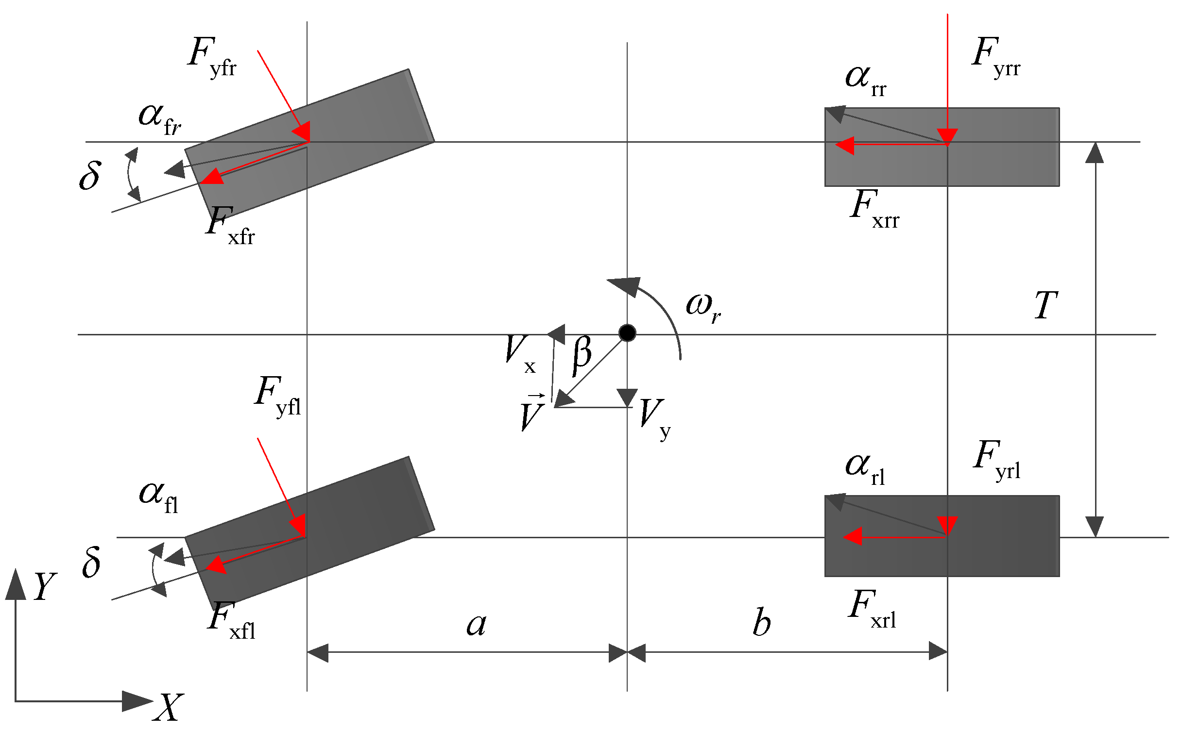
Figure 2.
The Diagram of the hierarchical MPC controller.
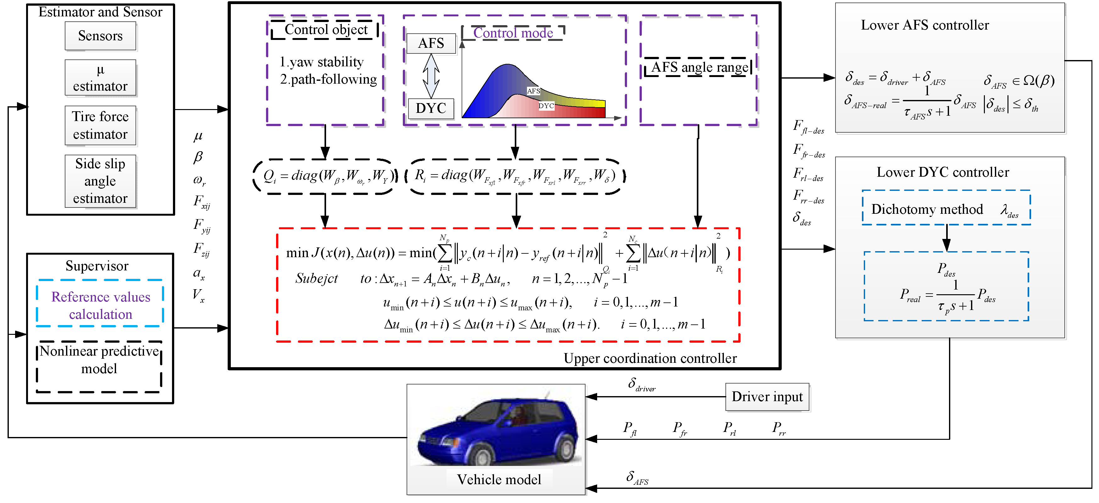
Figure 3.
The diagram of the Direct yaw moment control (DYC) and active front steering (AFS) working regions.
Figure 3.
The diagram of the Direct yaw moment control (DYC) and active front steering (AFS) working regions.
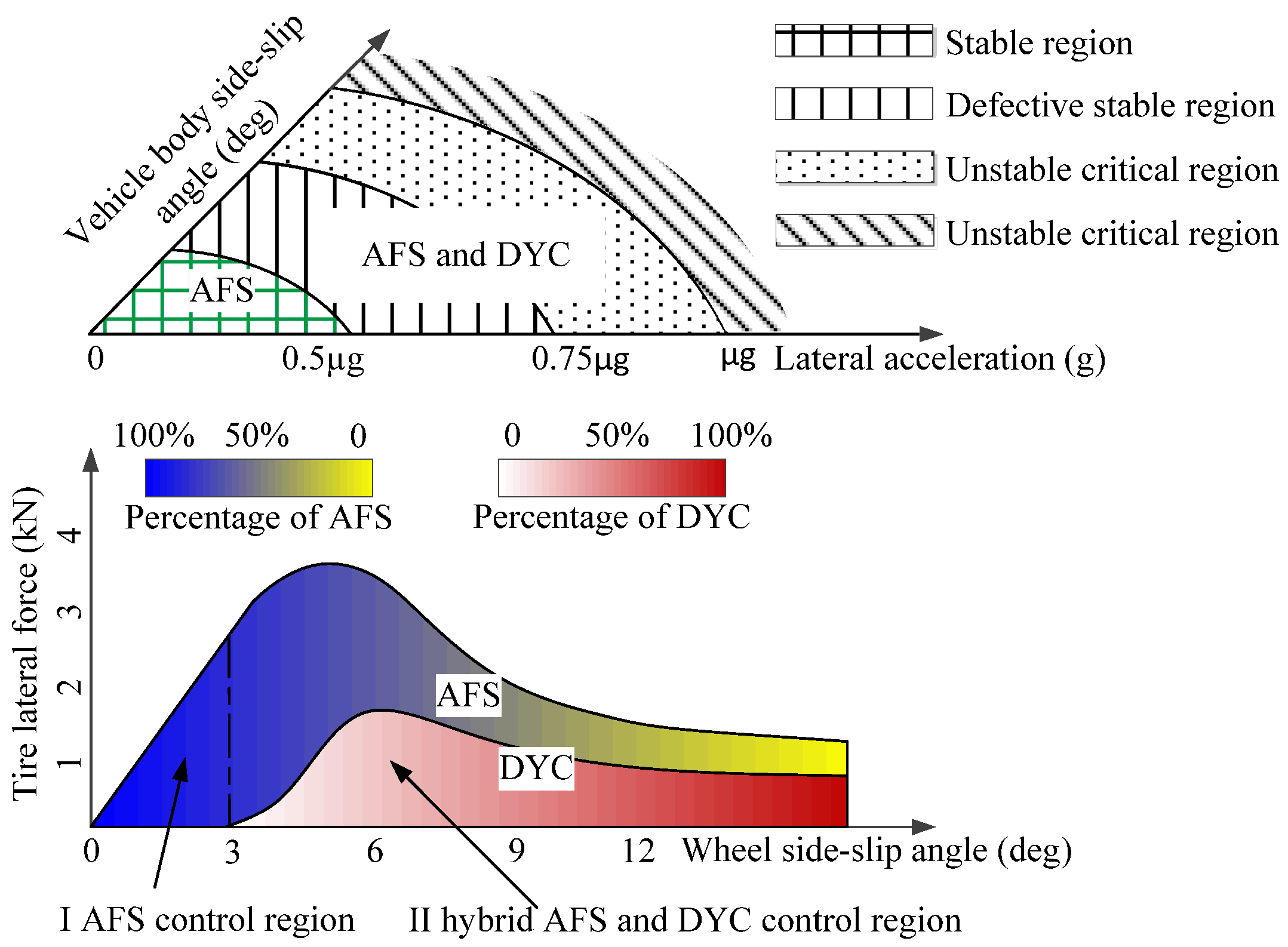
Figure 4.
The AFS additional angle range.

Figure 5.
The simulation flowchart of CarSim-MATLAB co-simulation.

Figure 6.
The steering wheel angles and longitudinal velocities with different controllers, (a) steering wheel angles; (b) longitudinal velocities.
Figure 6.
The steering wheel angles and longitudinal velocities with different controllers, (a) steering wheel angles; (b) longitudinal velocities.

Figure 7.
Comparison of the side slip angle, (a) HMCDC; (b) DYC controller.
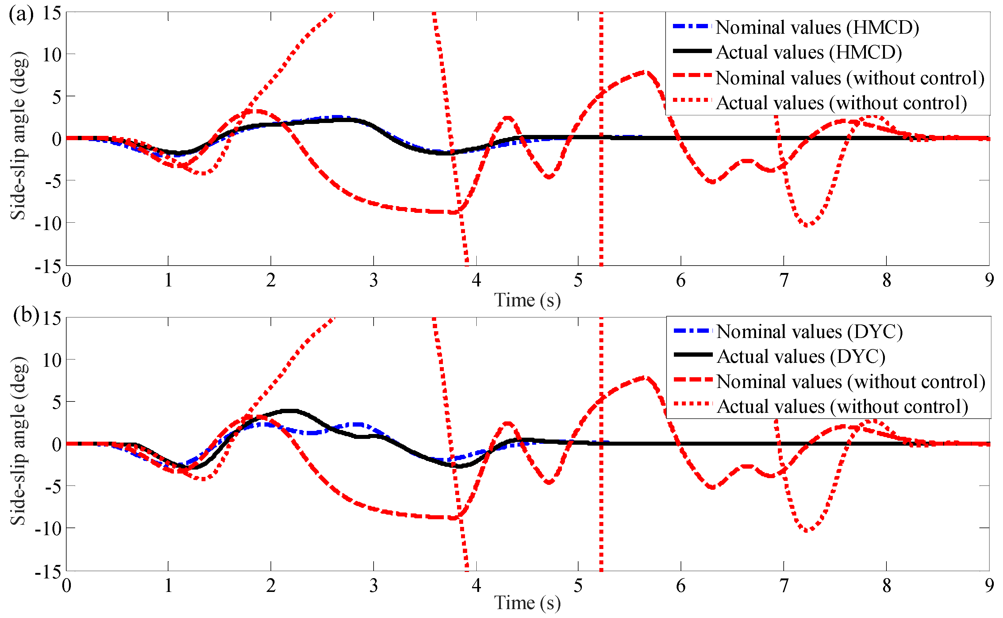
Figure 8.
Comparison of the yaw rate with different controllers, (a) HMCDC; (b) DYC controller.
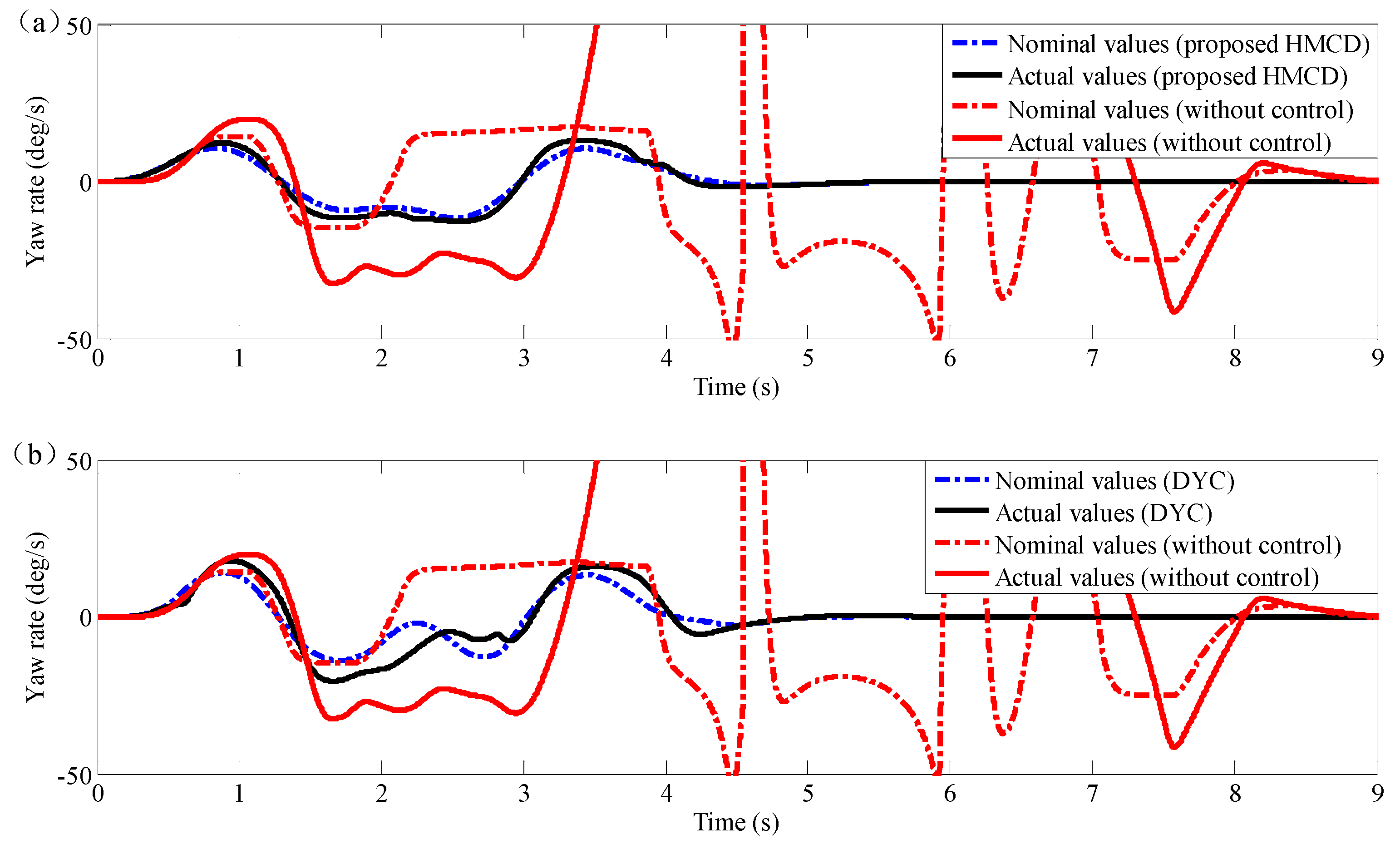
Figure 9.
The lateral accelerations and trajectories with different controllers, (a) trajectories; (b) lateral accelerations.
Figure 9.
The lateral accelerations and trajectories with different controllers, (a) trajectories; (b) lateral accelerations.
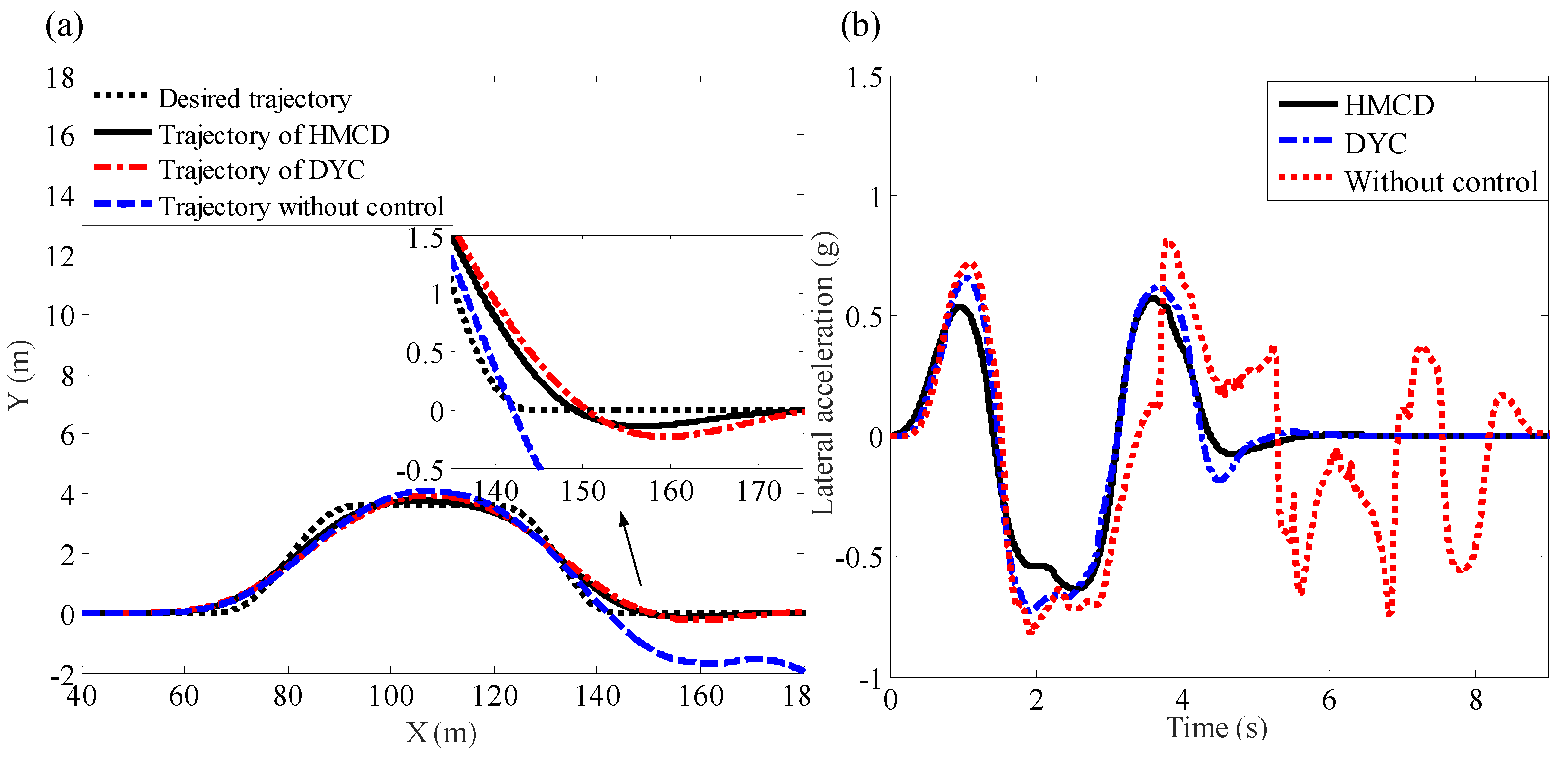
Figure 10.
The outputs of different controllers, (a) front wheel angle with HMCDC; (b) brake pressure of DYC; (c) brake pressure of HMCDC.
Figure 10.
The outputs of different controllers, (a) front wheel angle with HMCDC; (b) brake pressure of DYC; (c) brake pressure of HMCDC.

Figure 11.
The CF values controlled by different controllers and the CF threshold, (a) CF values; (b) limits of AFS additional angle.
Figure 11.
The CF values controlled by different controllers and the CF threshold, (a) CF values; (b) limits of AFS additional angle.
© 2017 by the authors. Licensee MDPI, Basel, Switzerland. This article is an open access article distributed under the terms and conditions of the Creative Commons Attribution (CC BY) license (http://creativecommons.org/licenses/by/4.0/).
Share and Cite
MDPI and ACS Style
Wu, J.; Cheng, S.; Liu, B.; Liu, C. A Human-Machine-Cooperative-Driving Controller Based on AFS and DYC for Vehicle Dynamic Stability. Energies 2017, 10, 1737. https://doi.org/10.3390/en10111737
AMA Style
Wu J, Cheng S, Liu B, Liu C. A Human-Machine-Cooperative-Driving Controller Based on AFS and DYC for Vehicle Dynamic Stability. Energies. 2017; 10(11):1737. https://doi.org/10.3390/en10111737
Chicago/Turabian StyleWu, Jian, Shuo Cheng, Binhao Liu, and Congzhi Liu. 2017. "A Human-Machine-Cooperative-Driving Controller Based on AFS and DYC for Vehicle Dynamic Stability" Energies 10, no. 11: 1737. https://doi.org/10.3390/en10111737
Note that from the first issue of 2016, this journal uses article numbers instead of page numbers. See further details here.