Advanced Wind Speed Prediction Model Based on a Combination of Weibull Distribution and an Artificial Neural Network

Abstract

One of the most crucial prerequisites for effective wind power planning and operation in power systems is precise wind speed forecasting. Highly random fluctuations of wind influenced by the conditions of the atmosphere, weather and terrain result in difficulties of forecasting regardless of whether it is short-term or long-term. The current study has developed a method to model wind speed data predictions with dependence on seasonal wind variations over a particular time frame, usually a year, in the form of a Weibull distribution model with an artificial neural network (ANN). As a result, the essential dependencies between the wind speed and seasonal weather variation are exploited. The proposed model utilizes the ANN to predict the wind speed data, which has similar chronological and seasonal characteristics to the actual wind data. This model was applied to wind speed databases from selected sites in Malaysia, namely Mersing, Kudat, and Kuala Terengganu, to validate the proposed model. The results indicate that the proposed hybrid artificial neural network (HANN) model is capable of depicting the fluctuating wind speed during different seasons of the year at different locations.

1. Introduction

Wind power is the most promising renewable energy and is one of the fastest developing electric generating technologies in the whole world [1]. Consequently, the pervasiveness of wind power in power systems has increased over the years. Figure 1 shows the global installed wind power capacity around the world, between 2000 and 2015. By the end of 2015, a total of 432.419 MW of capacity had been installed worldwide [2].

Wind power has an interesting resource potential as well as technology and is extensively utilized when considering energy mix options. Analysis of wind data characteristics and accurate wind power potential assessment at a given location is an imperative requirement before making a decision for the installation of a wind energy conversion system (WECS), as well as for assessing plans for connecting these projects with electrical power grids, or applications in remote areas.

For the effective development of wind power, the first measure for the electric utility is to conduct an adequate survey of wind availability. However, reliable wind speed data specifically for wind resource estimation is difficult to obtain [3,4]. Therefore, particular wind speed models are developed from the available wind speed data records that have been previously collected.

To predict wind speed, several approaches have been examined which can be categorized into four types [5]: (a) physical models; (b) statistical models; (c) artificial models; and (d) spatial correlation models. Each type of prediction model has its own specific characteristics. Compared to physical models, statistical models are typically simple and more appropriate for small farms [6]. The performance of hybrid models is usually better than that of single models, in wind speed forecasting [7]. This paper proposes a hybrid model that is a combination of the statistical model and the artificial neural network (ANN), which can effectively predict wind speed.

Wind speed forecasting has been investigated in some studies as reported [8,9]. The artificial neural network (ANN) is a potential technology in wind speed prediction. Li et al. [10] employed three types of feed-forward neural networks for accurate wind speed forecasting. Li et al. [11] developed an ANN-based methodology that provides a one-step-ahead prediction, and it demonstrated commendable performance in situations where there was no violent wind data oscillation.

A statistical time series analysis model involves constructing a model that is a representation of a time series; with this model, it is possible to predict the future values only from the distribution of past wind speed data values, and based on these distributions it can determine the special parameters of these distributions. According to Fortuna et al. [12], the time series data are characterized by time-varying data. The major time series clustering approaches can be categorized into three major groups, depending upon whether they work directly with raw data, indirectly with features extracted from the raw data, or indirectly with models built from raw data. Therefore, a significant assumption in the building of the time series model is stationary as a stationary time series can conveniently be reproduced by its mean value, standard deviation or variance.

In numerous recent studies, the Weibull distribution has been considered for expressing annual mean wind speed variation [13]. It represents various distribution characteristics when its parameter, shape and scale are appropriately tuned [14]. Therefore, the Weibull model can be applied for modeling wind speed changes and for forecasting future wind speeds [15,16].

The conventional modeling (statistical) approach is to fit the probability distribution to a given probability density function (PDF) model, and project statistical factors such as mean and variance [17]. However, these models do not have time variation properties and exclude cross-dependencies between other meteorological data. This current study has developed a method to model the wind speed data with dependence on seasonal wind variations over a particular time frame, usually a year, in the form of the Weibull model with ANN. As a result, the essential dependencies between the wind speed and seasonal weather variations are exploited. Both models were developed from three databases from three different sites in Malaysia, namely Mersing, Kudat, and Kuala Terengganu. The main objective was to compare the impact of the various meteorological variables on the performance of the Weibull model to determine whether it gave more efficient results. The results indicate that the proposed hybrid artificial neural network (HANN) model is capable of depicting the fluctuating wind speed during seasons of the year for different locations.

2. Related Work

2.1. Weibull Distribution

The Weibull model is only used with time series data, which is the normal distribution for the data, but with no representation of monsoon wind speed and seasonal weather components, as it is stationary. The time series wind speed model is a series of numerical observations from values of a wind speed measurement. These are normally regular observations (hours, days, months, years), but the sampling generated may be irregular or not, and as such, there is a need to predict the wind speed for the next hour or day. Therefore, the Weibull model is a suitable representation of the wind speed data distribution but is inadequate in simulating wind speed during the wind power potential models or for reliability assessment models [18], etc. The most obvious disadvantage of the Weibull probabilistic model is that the chronological characteristics of wind speed and its impact on wind power output are not reflected, thus the Weibull model is unable to consider both diurnal and seasonal wind speed variations [19].

In various recent studies, the Weibull distribution has been employed to represent the hourly variation of average wind speed over a year. At a specific wind site, the available electricity generated by a wind turbine depends on the mean wind speed and its standard deviation. Since yearly variation of annual mean wind speed is difficult to predict, wind speed variation can be well characterized in terms of a PDF [20]. The Weibull probability distribution function can be explained by the following Equation (1):

$$f\left(v\right)=\left(\frac{k}{c}\right){\left(\frac{v}{c}\right)}^{k-1}\exp [-{\left(\frac{v}{c}\right)}^k]$$

(1)

where f(v) is the probability of occurrence of wind speed v(v ≥ 0); c(c > 0) is the Weibull scale parameter; and k(k > 0) is the Weibull shape parameter. The complementary cumulative Weibull distribution function F(v) gives the probability of the wind speed exceeding the value v. The expression is given by the following Equation (2):

$$F\left(v\right)=\exp [-{\left(\frac{v}{c}\right)}^k]$$

(2)

The cumulative distribution function F(v) of the speed v gives the fraction of time (or probability) that the wind speed is equal or lower than v. Thus the cumulative distribution F(v) is the integral of the probability density function. It is also given by:

$$F\left(v\right)=1-\exp [-{\left(\frac{v}{c}\right)}^k]$$

(3)

In order to model the wind speed, the most commonly used method in power system simulation for random variable generation is the inverse transform of PDF [1]. Thus, the wind speed is simulated by combining the Weibull distribution and random variables.

Assume:

$$U=F\left(v\right)=1-\exp [-{\left(\frac{v}{c}\right)}^k]$$

(4)

where U is the uniformly distributed random variable between [0, 1]. Using the inverse transform method as shown in Equation (5):

$$v=c[-\ln {\left(1-U\right)}^{\frac{1}{k}}]$$

(5)

Since any (1 − U) also represents a random variable uniformly distributed between [0, 1], then Equation (5) can be simplified:

$$v=c[-\ln {\left(U\right)}^{\frac{1}{k}}]$$

(6)

Therefore, the speed of wind v can be generated artificially using Equation (6).

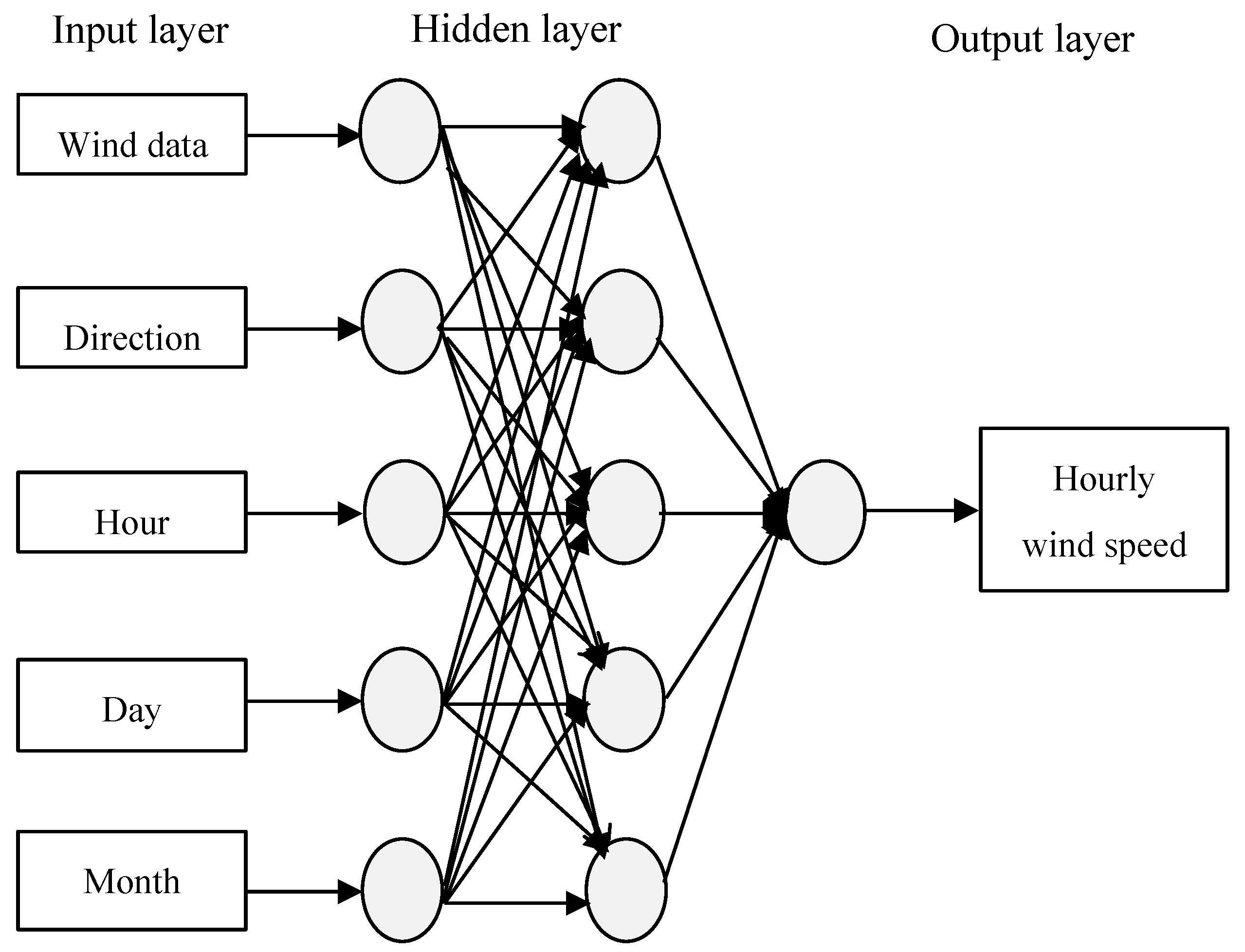
2.2. Description of the ANN Model

An ANN comprises some very simple and closely interconnected processors known as neurons [21], which are connected by weighted links that transmit signals from one neuron to another. Each link has an associated numerical weight. A neural network learns through repeated adjustments of these weights. The computational capabilities depend on the connection weights, network design, and training algorithms. An ANN has been used in various scientific and technological fields such as in predicting various environmental parameters including wind speed for wind power estimation [22]. An ANN derives information from data for the development of a complex relationship between input and output. Following the multiplication of the input variables by connection weights and the products, biases are added and passed through transfer functions to generate the output. The ANN is determined by the architecture, existing function, and training algorithms. The architecture influences its connection pattern among the neurons. In the process of training, the values of connection weights and biases are brought up to date to reduce the mean square of output error.

3. Proposed Model

The proposed model effectively integrates the Weibull model and ANN technique for short term wind speed prediction. The purpose of the HANN model is to improve the performance of the Weibull model to a level of high accuracy. In such hybrid methods, variations of seasonal characteristics are considered.

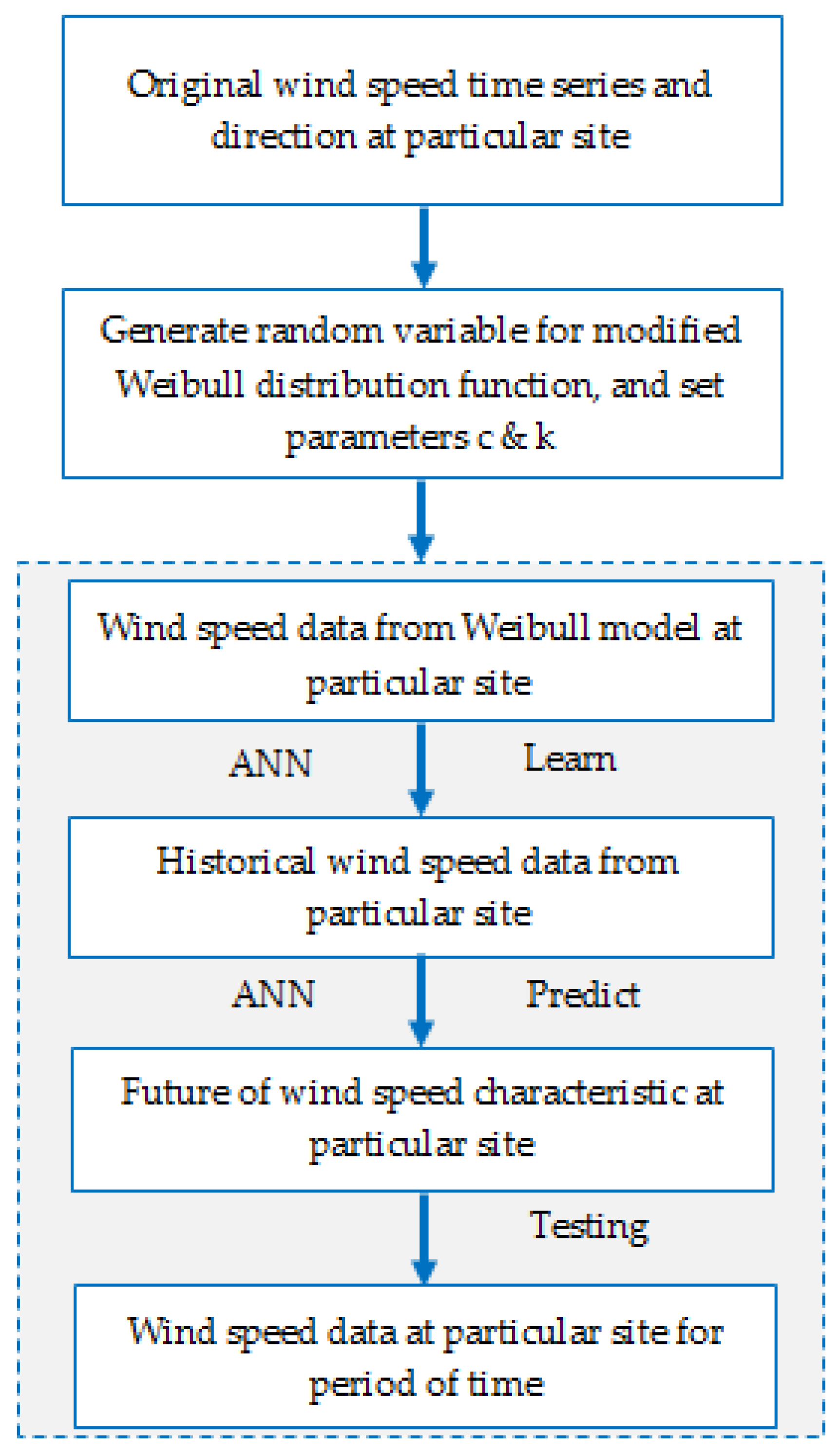
3.1. Description of the ANN Prediction Model

The input of the ANN model for wind speed prediction is the time series wind speed data generated by the Weibull model. In addition to direction, hour, day, month, and wind speed, as presented in Figure 2, the wind speed data values are taken from the MMD database.

The ANN fitting tool is employed to predict hourly wind speed for different sites. The fitting tool comprises a two-layer feedforward neural network. The Levenberg–Marquardt (LM) algorithm is utilized in static fitting problems for training, which is done automatically with scaled conjugate gradient even if the dataset is very large and performance is measured by employing mean square error and regression analysis. The output and target data are mapped in the range of -1 to 1. The data are randomly separated into 60% training, 20% testing and 20% validation. The training data adjusts the network weight based on error. The validation data evaluates network generalization and halts training when generalization ceases to improve. The testing data does not affect training and provides an independent indicator of network performance during and after training. The hidden layer neurons are obtained with the following expression:

$$H_n=\frac{I_n+O_n}{2}+\sqrt{S_n}$$

(7)

where H_n and S_n are the numbers of hidden layer neurons and number of data samples used in the ANN model, and I_n and O_n are the number of input and output parameters [23].

The training automatically ceases when generalization stops improving as demonstrated by an increase in the mean square error of the validation data samples. Repeated training times produce varying results because of the different initialization of connection weights.

3.2. Description of the Weibull Distribution Model

Weibull distribution can be shaped to represent many distributions by changing its parameters, as long as they are positive. The value of the scale parameter c of Weibull is close to the mean wind speed in actual data, and due to this, the Weibull distribution is a reasonable fit for data. Very often, when the k value is less or equal to two, both the Weibull and Rayleigh distributions are useful for representing the wind speed data distribution [24]. Weibull distribution can be used to model wind speed by properly setting the scale and shape to fit the given experimental data.

Many numerical methods are employed to estimate the values of the shape parameters k and scale c. The Empirical Method (EM) is used in this paper for estimating the Weibull parameters. The empirical method is considered a special case of the moment method, which can be obtained using its standard deviation and the mean wind speed, where the Weibull parameters c and k are given by the Equations (8) and (9) as shown below [25]:

$$k={\left(\raisebox{1ex}{$\sigma $}\!\left/ \!\raisebox{-1ex}{$⊽$}\right.\right)}^{-1.089}$$

(8)

$$c=\frac{⊽}{┌\left(1+\raisebox{1ex}{$1$}\!\left/ \!\raisebox{-1ex}{$k$}\right.\right)}$$

(9)

where $\sigma$ is the standard deviation; $⊽$ is the mean wind speed; $┌$ is the gamma function; and k can be determined easily from the values for $\sigma$ and $⊽,$ which are computed from the wind speed data set provided. Once k is obtained from the solution of the above numerical expression, the scale factor c can be calculated by the above equation.

The following are the major steps used in implementing the procedures for the simulation of the wind speed:

• Set the Weibull distribution parameters’ shape and scale.
• Generate a uniformly distributed random number U between [0, 1].
• Generate the random variable with the inverse transform of the modified cumulative Weibull distribution function as in Equation (3).
• Generate the artificial wind speed v with Equation (6).

Applying the Weibull distributed function using Equation (6), with the Weibull parameters c and k, which are deduced from the specific wind site. The simulated artificial wind speed profile for a given period can be conducted. From the simulation, it can be seen that the wind speed generated by the Weibull model is constantly changing; strong winds and weak winds are rare.

3.3. Procedures for the Integrated Model

In this model, the HANN algorithm is trained with the help of the historical wind speed data from a specific site. All simulation works and coding was performed using various software such as Matlab (neural net fitting tools) and WRPLOT View 7.0 ©1998–2011 Lakes Environmental software. Figure 3 shows the overall procedures involved in the simulation and prediction of the wind speed data by using the HANN model, which can be summarized in three steps as follows:

• Firstly, the fitting of the Weibull parameters to randomly create the hourly wind speed.
• Secondly, applying the ANN to intensify the hourly wind speed data to match the characteristics of the actual wind speed data.
• Thirdly, the period of prediction is based on the required period of time generated.

3.4. Analysis of the Prediction Error

To assess the proposed HANN model, two error statistics were taken into consideration, the mean absolute percentage error (MAPE) and root mean square error (RMSE) [26]. The MAPE indicates the accuracy in fitting time series values in statistics, in particular, trending. The wind speed prediction accuracy is established by MAPE, which characteristically presents accuracy as a percentage, and is defined by the formula [27]:

$$\mathrm{MAPE}=\frac{1}{n}{{\displaystyle \sum }}_{t=1}^n\frac{y_{i\left(ANN\right)}-y_{k\left(measured\right)}}{y_{k\left(measured\right)}}$$

(10)

where n is the total number of input and output pairs used for training; $y_{i\left(ANN\right)}$ is the forecast wind speed for one hour; and $y_{k\left(measured\right)}$ is the actual wind speed for one hour.

A MAPE < 10% indicates high prediction accuracy, 10% ≤ MAPE ≤ 20% indicates good prediction, 20% ≤ MAPE ≤ 50% implies acceptable prediction, and MAPE ≥ 50% implies inaccurate prediction [23]. On the other hand, RMSE demonstrates the efficiency of the developed ANN in projecting future individual values, a large positive RMSE indicates a considerable deviation in the predicted value from the real value.

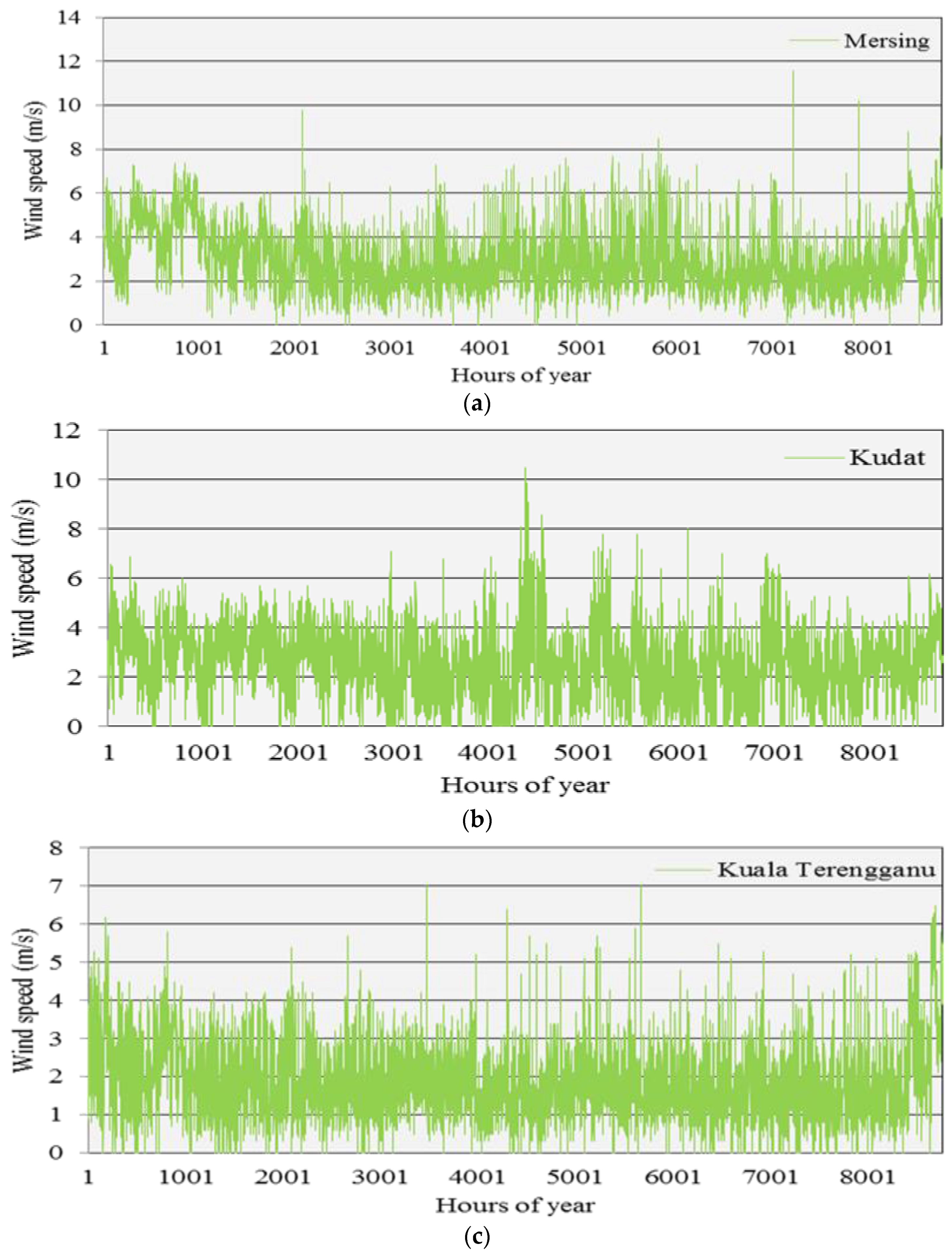
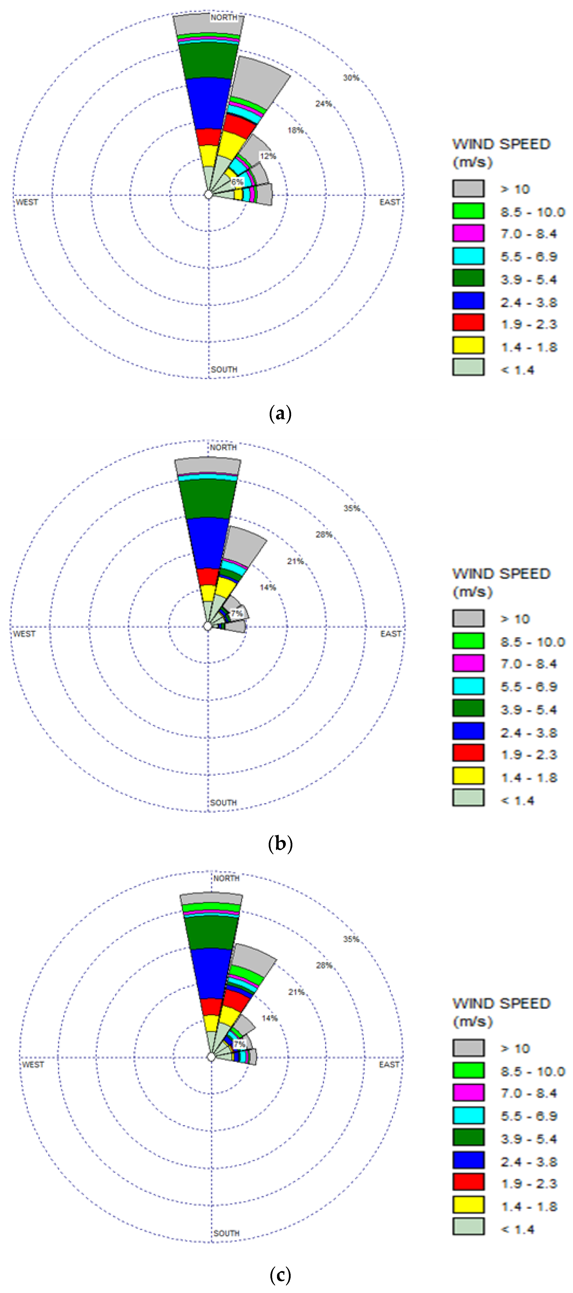
4. Wind Data Characteristics at Selected Locations in Malaysia

Malaysia is in the equatorial region in South East Asia, between northern latitude 1° N and 6° N and eastern longitude from 100° E to 109° E. The wind that blows across peninsular Malaysia is influenced by two monsoon seasons, namely the southwest monsoon from May to September, and the northeast monsoon from November to March. The two monsoons are interspersed by two short inter-monsoon periods [28].

The data for this study were gathered from the Malaysia Meteorological Department (MMD). The data records comprise over three years of hourly mean surface wind speed and direction from 1 January 2013 until 31 December 2015, at three locations in Malaysia.

Table 1. Description of the measured wind speed stations in regions in Malaysia.

Station	Latitude	Longitude	Altitude (m)
Mersing	2°27′ N	103°50′ E	43.6
Kuala Terengganu	5°23′ N	103°06′ E	5.2
Kudat	6°55′ N	116°50′ E	3.5

presents the description of the selected regions in Malaysia which consists of latitudes, longitudes, and the elevation of the anemometer.

In this study, the recorded hourly time series surface wind data in Mersing, Kudat, and Kuala Terengganu for the year 2015 were analyzed statistically. The monthly average wind speed values and the standard deviations for each site were calculated. The results of the mean wind speed is tabulated in

Table 2. Monthly mean wind speed and standard deviation of three sites in Malaysia.

Month/Year 2015	Mersing		Kudat		Kuala Terengganu
	⊽	$\mathit{\sigma }$	⊽	$\mathit{\sigma }$	⊽	$\mathit{\sigma }$
January	4.10	1.2809	3.08	1.2838	2.45	1.1840
February	4.13	1.4205	3.01	1.1849	2.21	1.1179
March	3.16	1.2627	3.13	1.1191	1.97	1.0388
April	2.59	0.9805	2.68	1.1232	1.80	0.8997
May	2.44	1.0748	2.09	1.3086	1.87	0.7819
June	2.74	1.2152	2.14	1.4235	1.71	0.8050
July	2.87	1.3338	2.54	1.6326	1.71	0.8031
August	3.02	1.4429	2.58	1.6159	1.81	0.8053
September	2.69	1.2636	2.04	1.3367	1.65	0.7898
October	2.64	1.1998	2.46	1.4856	1.63	0.8696
November	2.23	0.9127	2.11	1.1661	1.68	0.9186
December	3.31	1.5967	2.73	1.1498	2.42	1.3789
Annual mean	2.99	1.2487	2.55	1.3192	1.91	0.9494

.

To obtain a clearer picture of the actual wind speed of these three locations, the hourly variation of wind speed distribution is presented. Figure 4 shows the hourly wind speed recorded in Mersing, Kudat, and Kuala Terengganu throughout the year 2015.

The wind rose is helpful in determining the predominant wind of a location during the time period. On the basis of the observed wind speed data, the frequencies (%) are plotted in the chart with respect to the cardinal point to indicate the wind direction. It is evident that the direction of wind speed blowing in the same sites for years is characterized by a considerable stability, which is shown in Figure 5. The most likely wind direction for all the years and sites in Malaysia were prevailing winds blowing from a southwesterly to northeasterly direction.

5. Results and Discussion

5.1. Weibull Parameter Results

The estimation of wind speed data for the year 2015 at Mersing, Kudat, and Kuala Terengganu using a Weibull distribution is presented in this section. Consequently, the scale parameters were computed corresponding to the wind speed of the particular month in terms of the shape parameters of the month. The calculation of both Weibull parameters is shown in

Table 3. The values of the Weibull parameter estimation by Empirical Method at Mersing, Kudat, and Kuala Terengganu based on hourly wind speed data for the year 2015.

Month/Year 2015	Mersing		Kudat		Kuala Terengganu
	K	C	K	C	K	C
January	3.5527	4.5565	2.5979	3.4733	2.2034	2.7615
February	3.1998	4.6146	2.7640	3.3863	2.0979	2.4923
March	2.7192	3.5570	3.0682	3.5049	2.0084	2.2239
April	2.8760	2.9018	2.5796	3.0197	2.1309	2.0350
May	2.4439	2.7535	1.6682	2.3432	2.5826	2.1043
June	2.4242	3.0904	1.5626	2.3866	2.2781	1.9356
July	2.3027	3.2382	1.6193	2.8379	2.2806	1.9329
August	2.2365	3.4115	1.6677	2.8927	2.4141	2.0404
September	2.2803	3.0409	1.5864	2.2758	2.2342	1.8656
October	2.3599	2.9784	1.7338	2.7634	1.9767	1.8341
November	2.6516	2.5146	1.9072	2.3776	1.9279	1.8924
December	2.2129	3.7389	2.5681	3.0789	1.8415	2.7191
Average	2.60	3.37	2.11	2.86	2.16	2.15

for Mersing, Kudat, and Kuala Terengganu for the year 2015.

From the results, it can be observed that the value scale parameter c of Weibull is close to the actual mean wind speed. This is true as the Weibull distribution is a reasonable fit to the wind speed data. This analysis suggests that the Weibull distribution is the best distribution and offers a very beneficial model to predict potential wind energy.

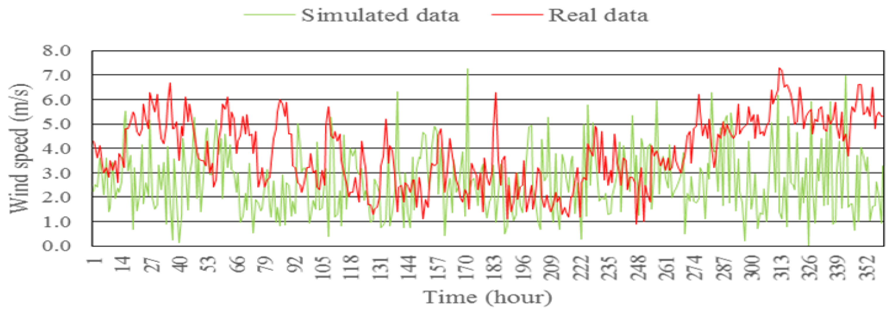
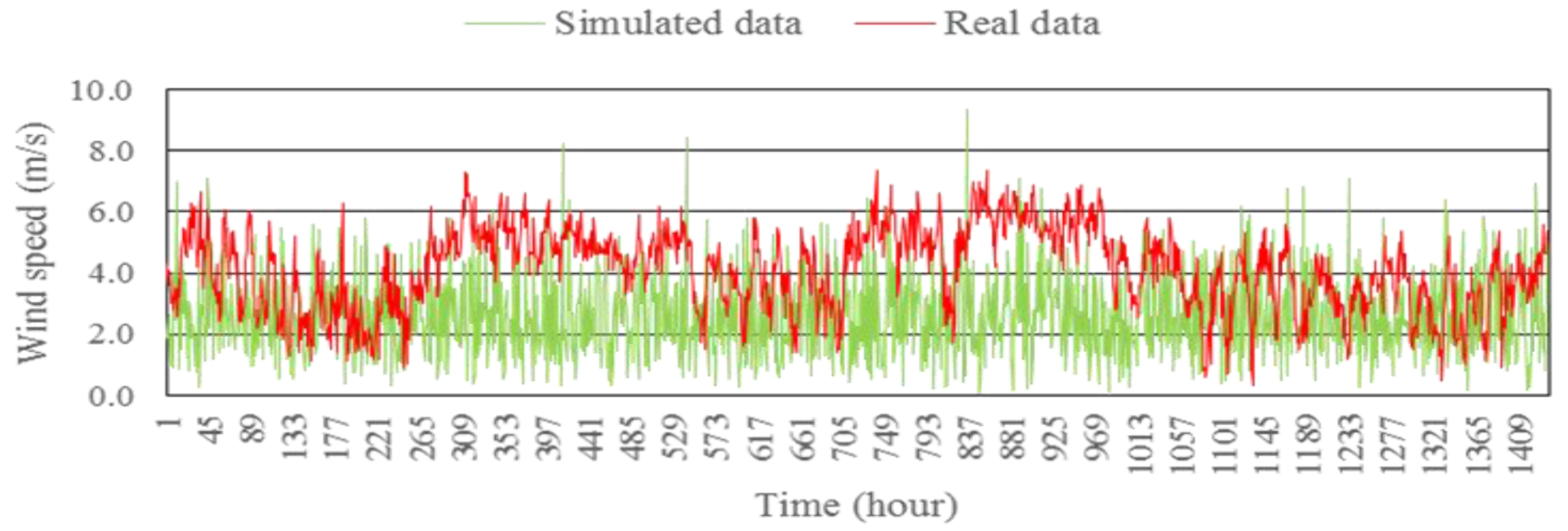
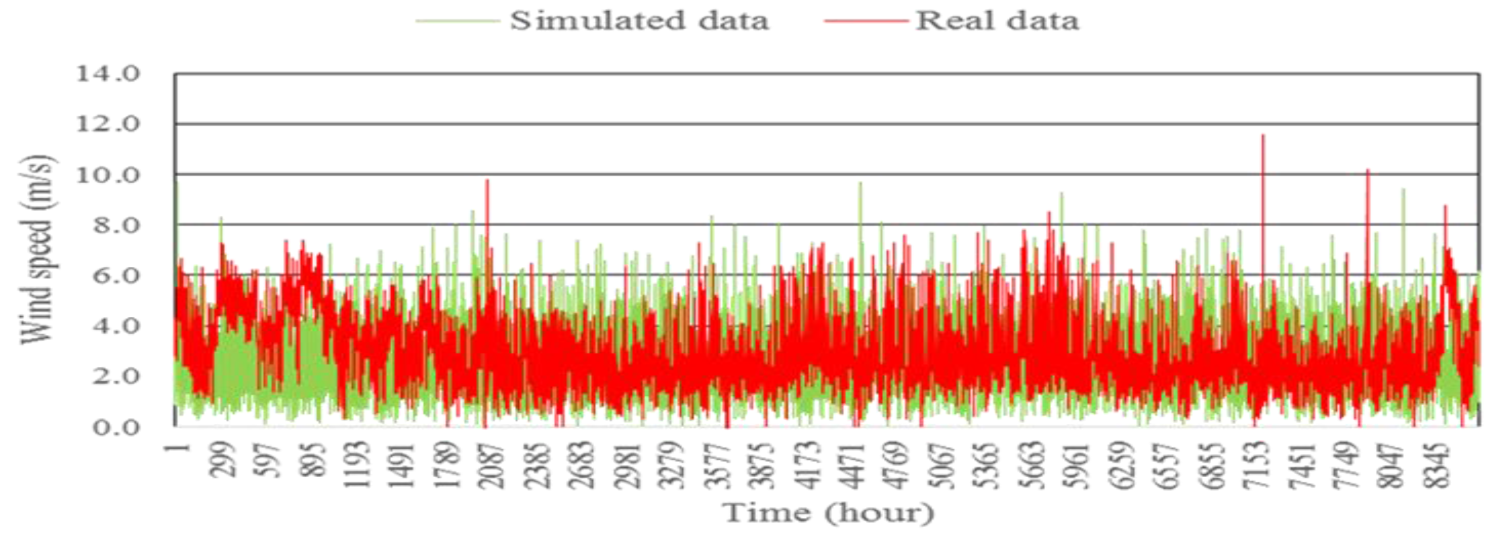
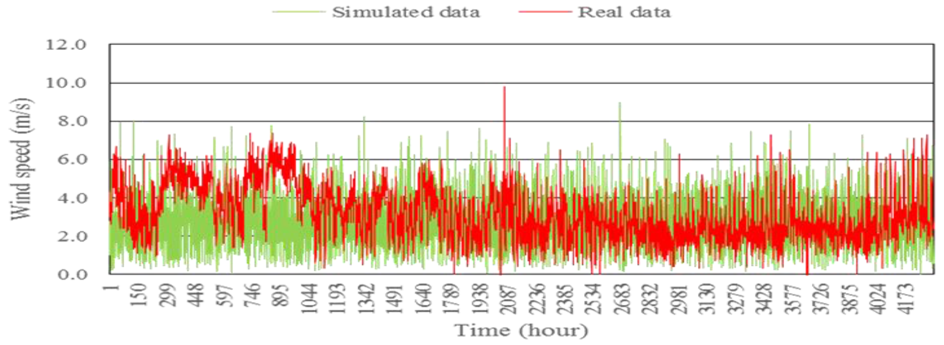
5.2. Weibull Model for the Prediction and Simulation of Wind Speed

The Weibull results for simulated wind speed data are illustrated in Figure 6, Figure 7, Figure 8 and Figure 9, in which are represented a comparison of hourly wind speed data generated using the Weibull model and real wind speed data. Figure 6, Figure 7, Figure 8 and Figure 9 show the simulation of wind speed time-series data with c = 3.37, and k = 2, for wind data collected at the Mersing site in 2015. As expected, this wind speed data is not similar to the actual wind speed data, which implies a very low predictability.

Firstly, Figure 9 shows a comparison between the measured data collected at the Mersing site for the year 2015 at a height of 43.6 m, with wind speed data generated by the Weibull model. From Figure 9, it can be seen that for the first two months, January and February (Mersing/2015), the simulated wind speed is not identical to the measured data for this location for the one-year data. While the average wind speed for the months of January and February, as shown in Table 2, is around 4.10 m/s and 4.13 m/s, respectively, the value of c, which represents the average wind speed for the Weibull model is around 3.37 m/s, as shown in Table 3. The difference between the values of mean wind speed and c value, suggests that the Weibull model does not take into consideration the seasonal variations in calculations during the year.

To avoid inaccuracy in the wind speed data created from the Weibull model, especially for the forecast of the wind speed data during the seasons which have higher wind speed, particularly during monsoon season, the HANN model was used to correct the wind speed data according to seasonal variations of wind speed during the year for the Mersing site.

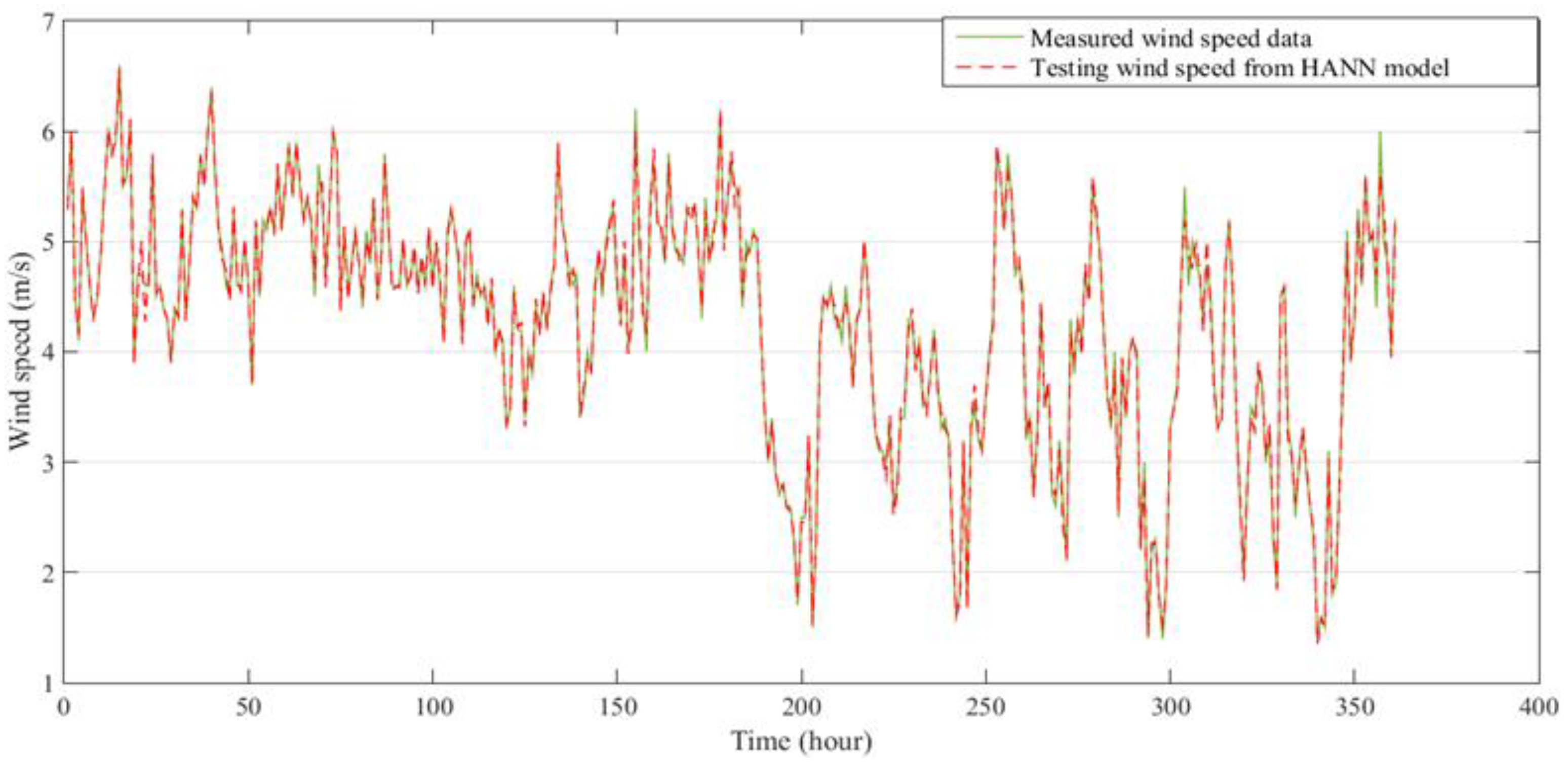
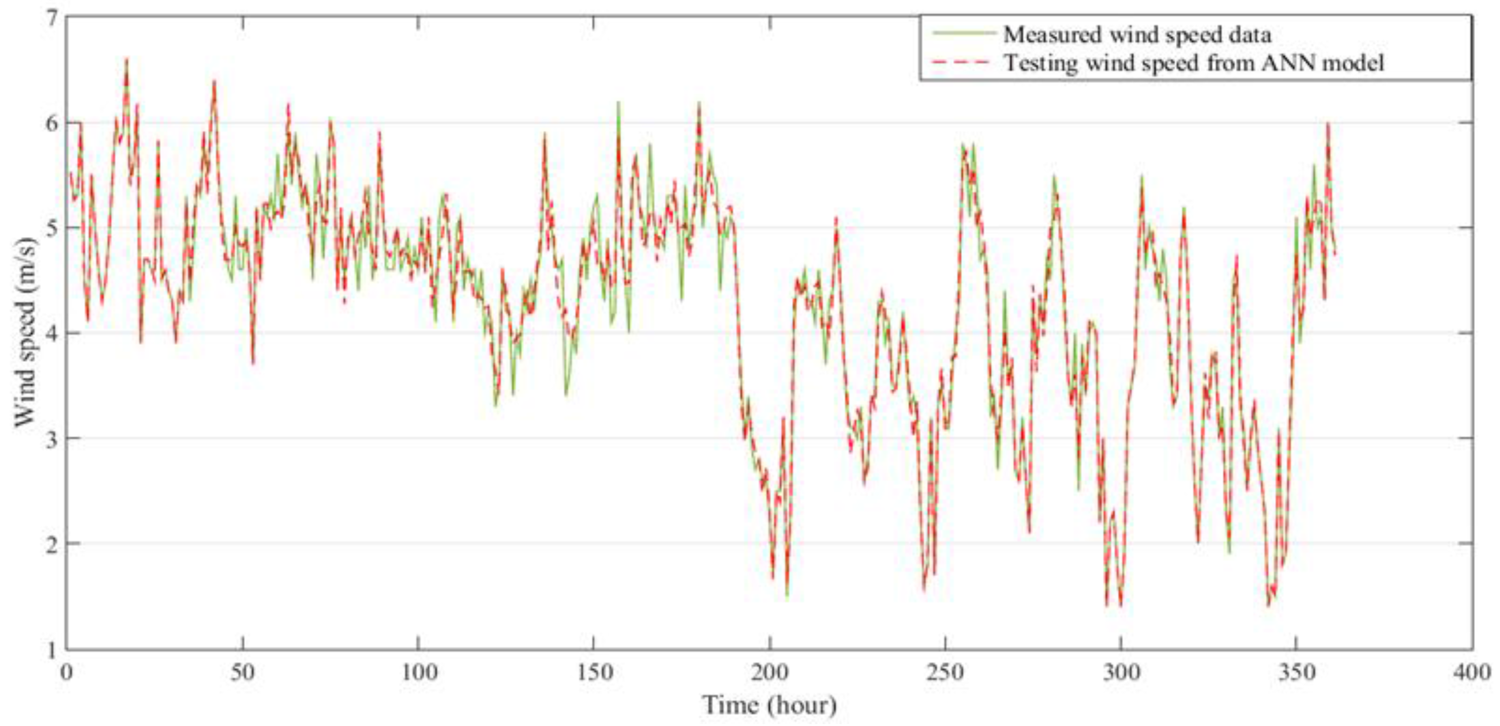
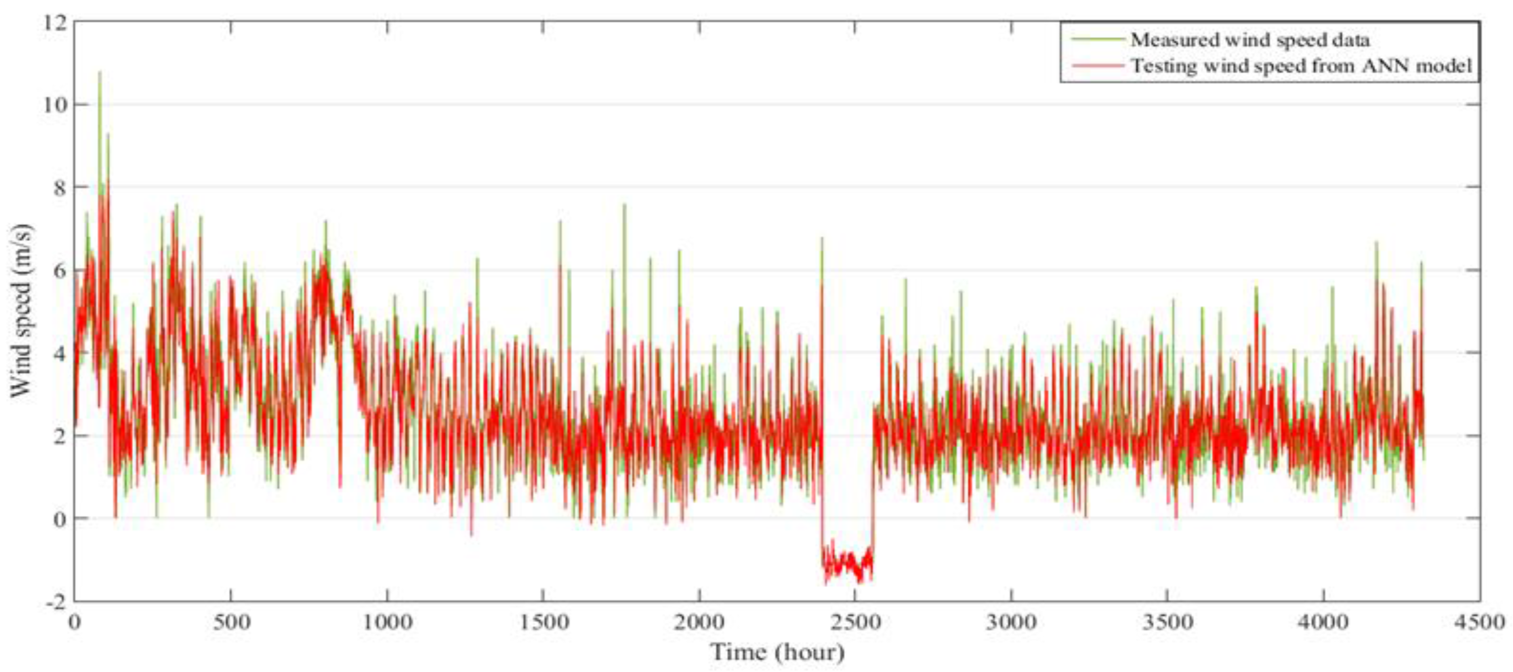
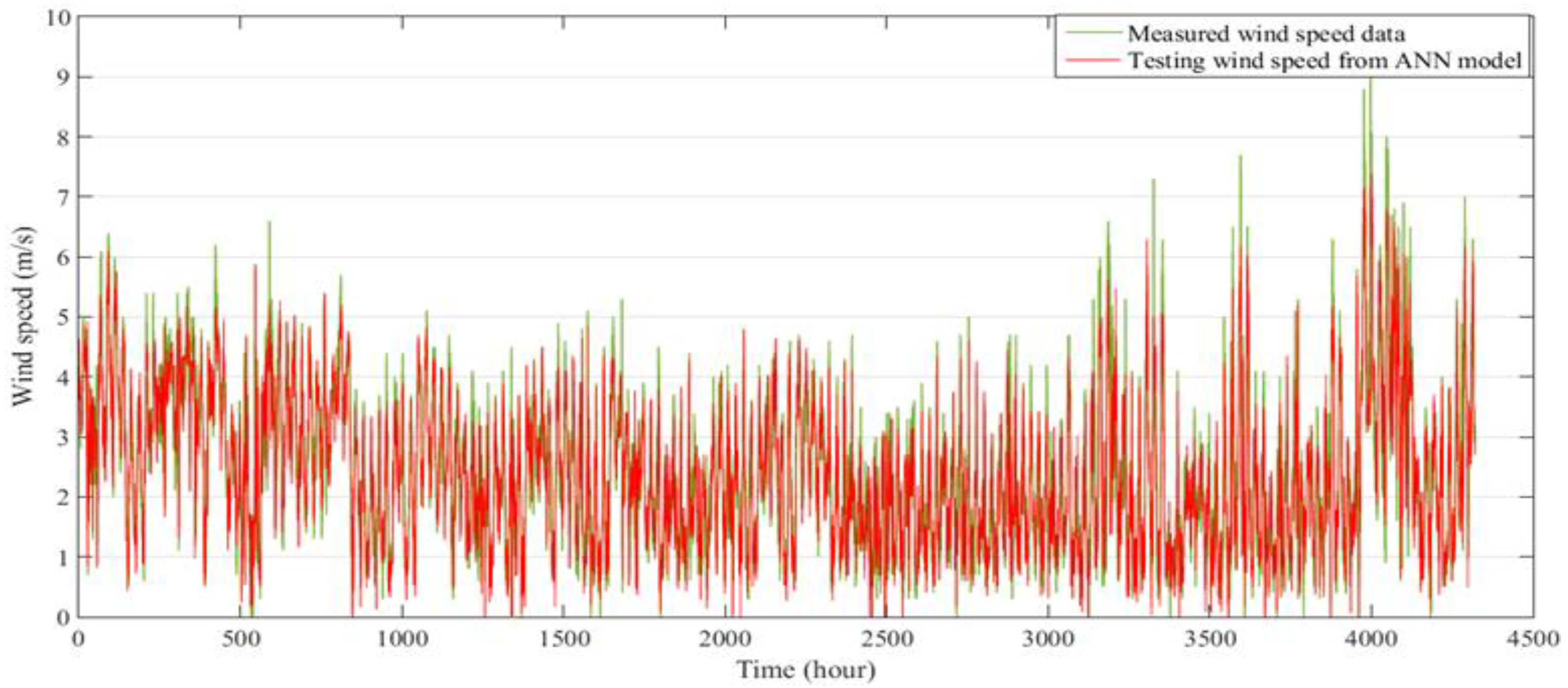
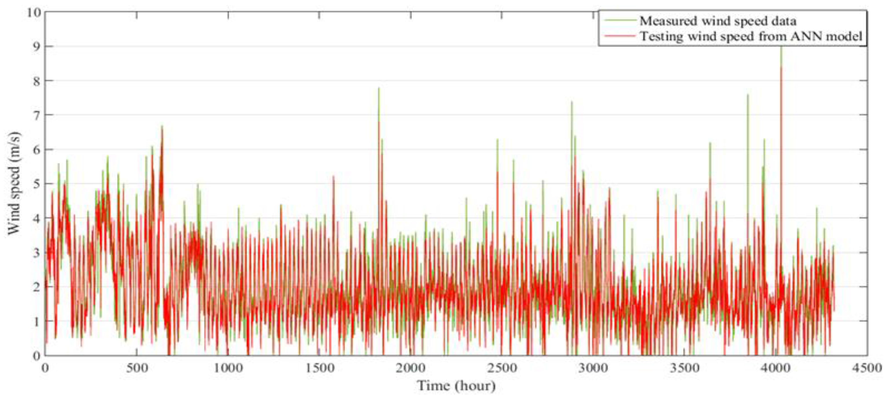
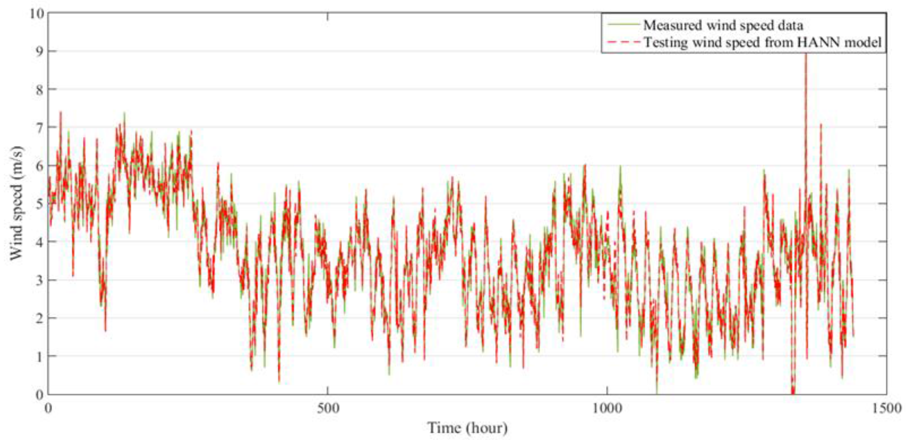
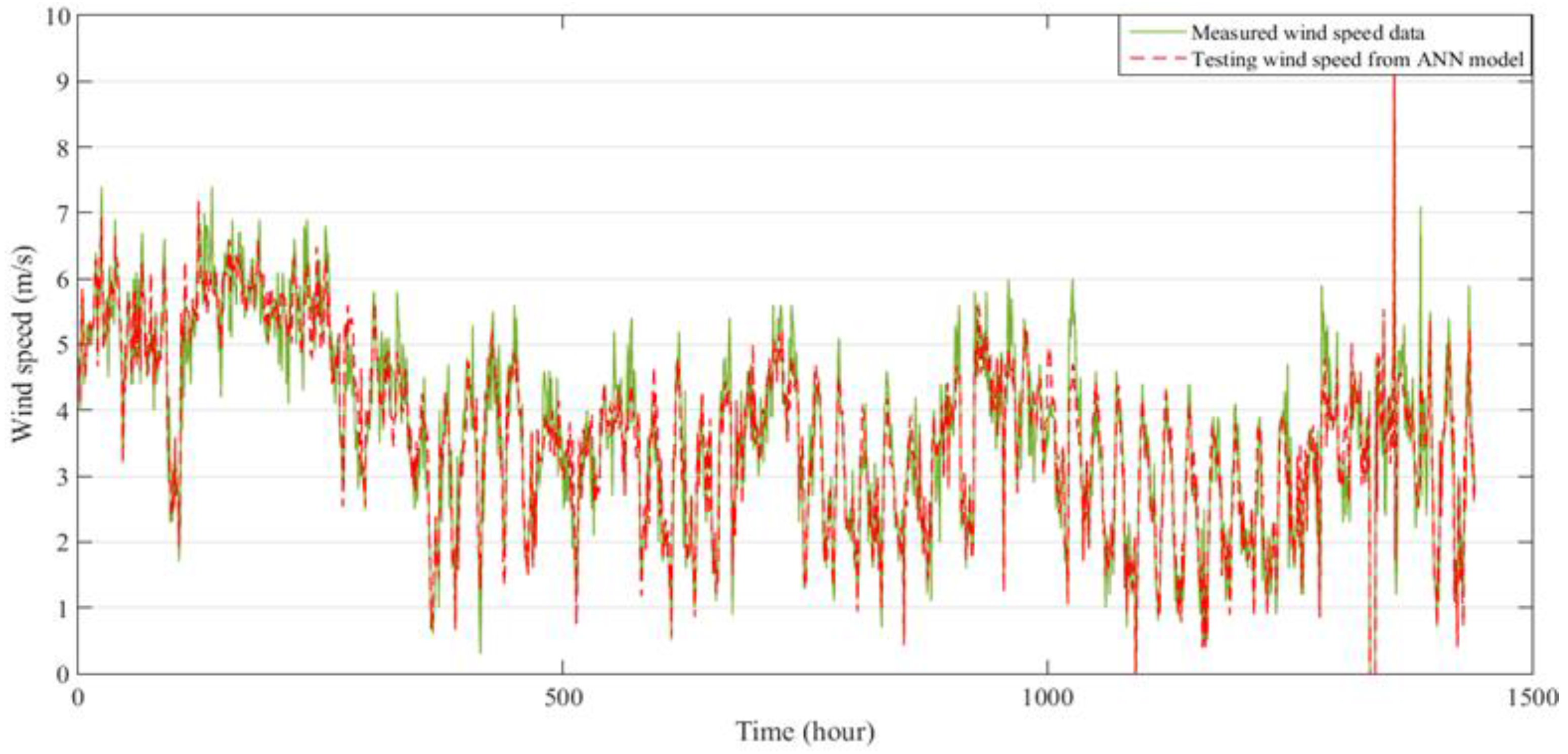
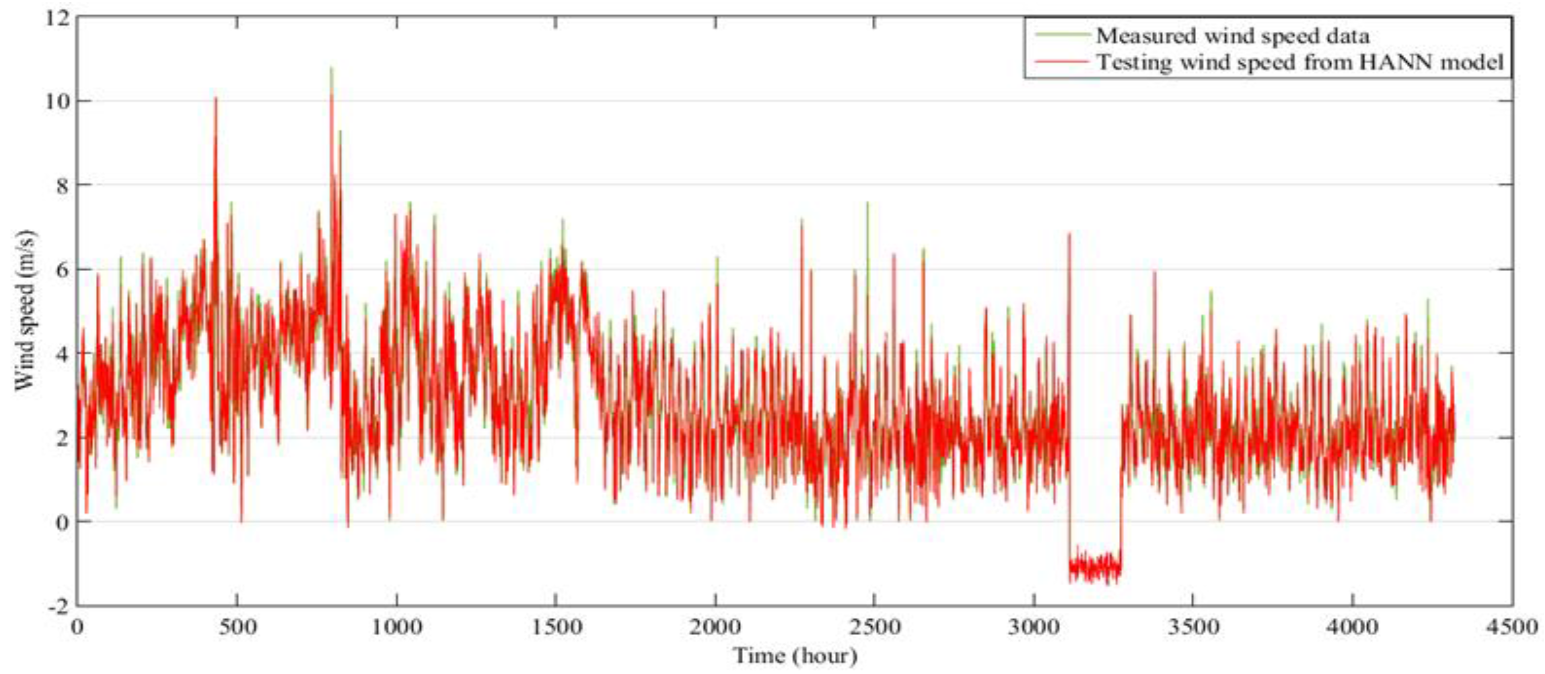
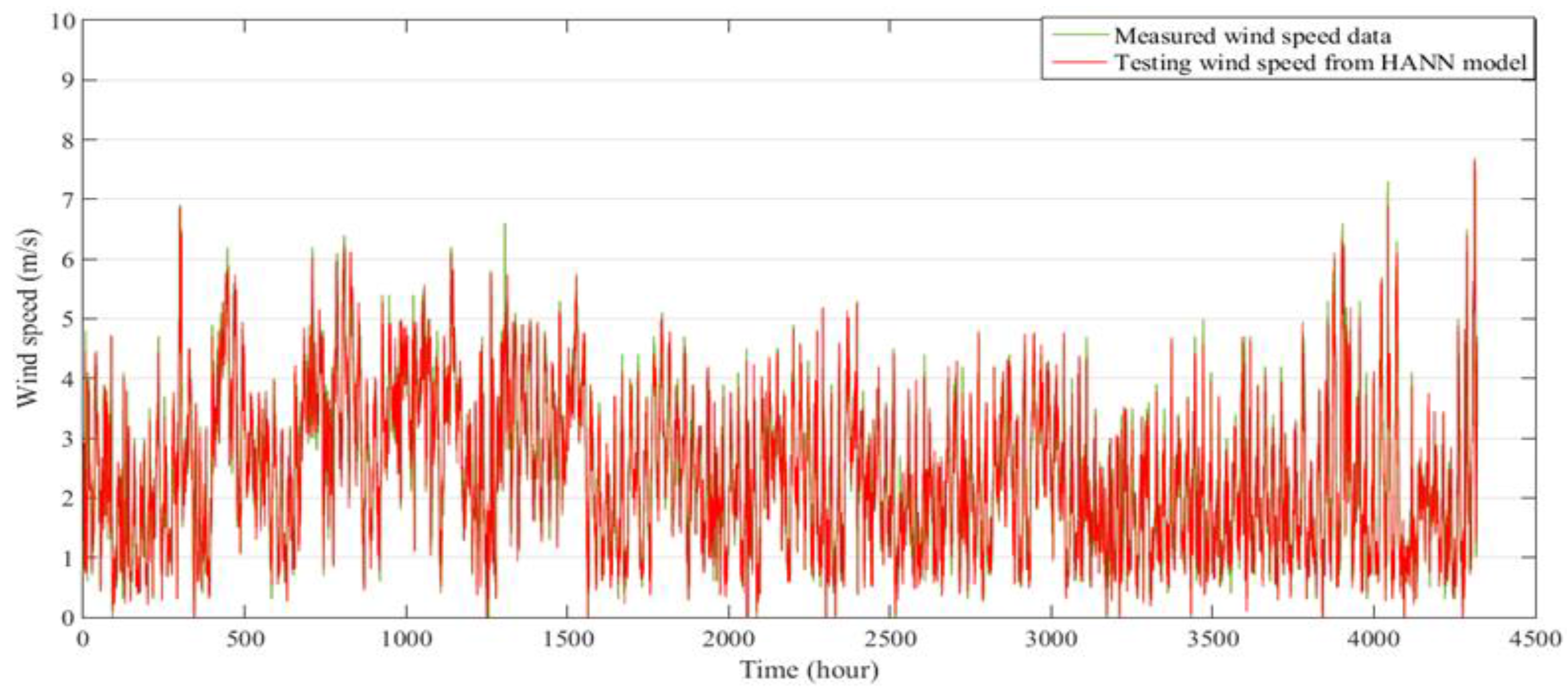
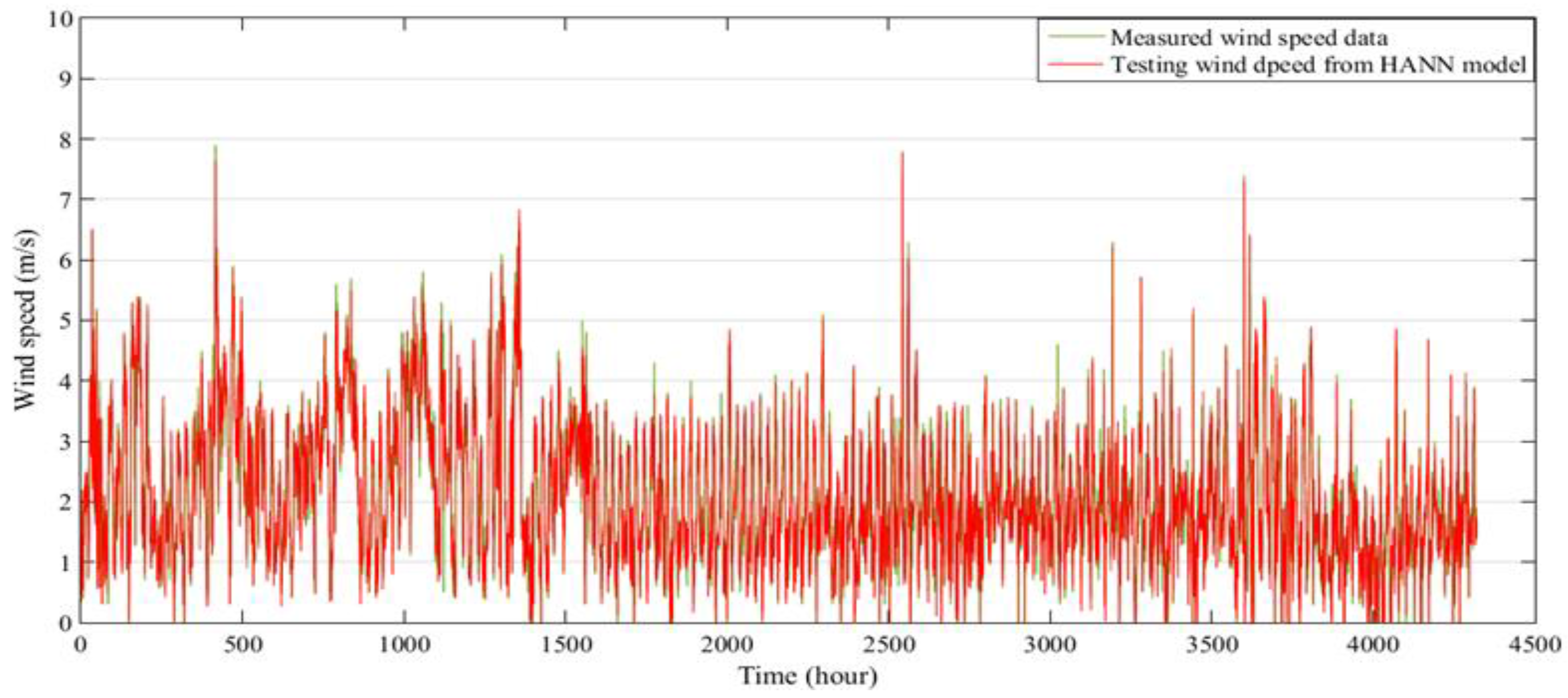
5.3. Implementation of the ANN Model and HANN Model for Validation of the Results

The proposed HANN model was applied to test the generated wind speed data from the Weibull model at the Mersing site. Figure 10 and Figure 11 show simulated wind speed data for the first two weeks in January and the first two months of the year, for wind speed data at Mersing in 2015.

Hourly wind speed data were used in this study to test the proposed HANN algorithm. Historical wind speed data collected from the Mersing site in 2015 were used as the input for the prediction-alone ANN algorithm in the training and in the test phases. Figure 12 and Figure 13 show the simulated wind speed data for the first two weeks in January and the first two months of the year, for wind speed data at Mersing in 2015.

The proposed HANN model was compared with the ANN model and Weibull model. This comparison demonstrated that the HANN model presents lower RMSE and MAPE for different horizons. The results of the proposed methods were compared in terms of MAPE and RMSE, for the Weibull model, ANN model, and HANN model, as shown in

Table 4. Statistical errors generated by the Weibull model, ANN model, and HANN model.

Mersing
Model	Two-Week		Two-Month
	MAPE	RMSE	MAPE	RMSE
Weibull model	0.880	1.650	1.575	2.429
ANN model	0.032	0.205	0.104	0.485
HANN model	0.014	0.081	0.065	0.259

. The values of MAPE and RMSE for two weeks from the first month of January, and two months of the year in Mersing in 2015, were 0.014 and 0.081, 0.065 and 0.259, respectively. The results from the HANN model for the simulation of the Mersing wind speed data showed high prediction accuracy.

Figure 14, Figure 15 and Figure 16 show the predicted wind speed data for the entire three years from 2013 to 2015 for the Mersing, Kudat, and Kuala Terengganu sites in Malaysia using the ANN model.

The results of the prediction of the wind speed using the proposed HANN model are plotted in Figure 17, Figure 18 and Figure 19. These results show the predicted wind speed data for the entire three years from 2013 to 2015, for the Mersing, Kudat, and Kuala Terengganu sites in Malaysia. The statistical errors obtained by using two models for predicting the wind speed data are presented in

Table 5. Statistical errors generated by the ANN model and the proposed HANN model.

Model	Mersing		Kudat		Kuala Terengganu
	MAPE	RMSE	MAPE	RMSE	MAPE	RMSE
ANN model	16.4%	0.492	20.3%	0.483	19.9%	0.426
HANN model	6.06%	0.048	8.06%	0.039	8.01%	0.034

.

From Table 5, it can be seen that the MAPE values for the six months of the year at Mersing, Kudat, and Kuala Terengganu using the ANN model were 16.4%, 20.3%, and 19.9%, respectively. The percentage values of the MAPE are within (10% ≤ MAPE ≤ 20%), which indicates good prediction for the six months wind speed data for the three sites [23].

Meanwhile, the MAPE values for the first six months of the year in Mersing, Kudat, and Kuala Terengganu using the HANN model, were 6.06%, 8.06%, and 8.01%, respectively. The percentage values of the MAPE are within (MAPE < 10%), which indicates high prediction accuracy for the six months wind speed data for the three sites.

The results of the simulation demonstrate that the proposed method is appropriate for forecasting both the hourly and daily wind series. The results obtained show that reasonable and good wind speed predictions can be made with the two parameters of the Weibull model and ANN model, respectively. However, using the HANN model produced more accurate results.

6. Conclusions

The current study developed a method to model the wind speed prediction while considering seasonal wind variations over a particular time frame, in the form of a hybrid model consisting of the Weibull and ANN model. Procedures for the prediction and simulation of the wind speed using a hybrid model are as follows: firstly, the fitting of the Weibull parameters to create hourly wind speed randomly; and secondly, applying the ANN to intensify the hourly wind speed data to match the characteristics of the actual wind speed data. Consequently, the forecasted errors of wind values are lower than those generated using only the Weibull model.

This model has been applied to wind speed data for sites in Malaysia, namely Mersing, Kudat, and Kuala Terengganu, to validate the proposed method. The results indicate that the proposed HANN model is capable of depicting the fluctuating wind speed during different seasons of the year for different locations. As a result, the essential dependencies between the wind speed and seasonal weather variations are exploited. The results show that the predicted wind speed data has similar chronological and seasonal characteristics to the actual wind data.

Recommendations for future studies include employing the proposed model with probabilistic methods for a reliability assessment of power systems with wind power integration.

References

1. Shuai, S.; Lo, K.L. An Overview of Wind Energy Development and Associated Power System Reliability Evaluation Methods. In Proceedings of the 48th International Universities Power Engineering Conference (UPEC), Dublin, Ireland, 2–5 September 2013; pp. 1–6. [Google Scholar]
2. Global Wind Energy Council. Global Wind Statistics 2015. Available online: http://www.gwec.net/ (accessed on 10 February 2016).
3. Anurag, C.; Saini, R.P. Statistical Analysis of Wind Speed Data Using Weibull Distribution Parameters Statistical Analysis of Wind Speed Data Using. In Proceedings of the 1st International Conference on Non-Conventional Energy (ICONCE2014), Kalyani, India, 16–17 January 2014. [Google Scholar]
4. Kidmo, D.K.; Danwe, R.; Doka, S.Y.; Djongyang, N. Statistical analysis of wind speed distribution based on six Weibull Methods for wind power evaluation in Garoua, Cameroon. Revue Des Energies Renouvelables 2015, 18, 105–125. [Google Scholar]
5. Liu, H.; Chen, C.; Tian, H.; Li, Y. A hybrid model for wind speed prediction using empirical mode decomposition and artificial neural networks. Renew. Energy 2012, 48, 545–556. [Google Scholar] [CrossRef]
6. Peng, H.; Liu, F.; Yang, X. A hybrid strategy of short term wind power prediction. Renew. Energy 2013, 50, 590–595. [Google Scholar] [CrossRef]
7. Liu, H.; Tian, H.; Li, Y. Comparison of two new ARIMA-ANN and ARIMA-Kalman hybrid methods for wind speed prediction. Appl. Energy 2012, 98, 415–424. [Google Scholar] [CrossRef]
8. Cadenas, E.; Rivera, W.; Campos-amezcua, R.; Heard, C. Wind speed prediction using a univariate Arima model and a multivariate NARX Model. Energies 2016, 9, 109. [Google Scholar] [CrossRef]
9. Okumus, I.; Dinler, A. Current status of wind energy forecasting and a hybrid method for hourly predictions. Energy Convers. Manag. 2016, 123, 362–371. [Google Scholar] [CrossRef]
10. Li, G.; Shi, J.; Zhou, J. Bayesian adaptive combination of short-term wind speed forecasts from neural network models. Renew. Energy 2011, 36, 352–359. [Google Scholar] [CrossRef]
11. Li, G.; Shi, J. On comparing three artificial neural networks for wind speed forecasting. Appl. Energy 2010, 87, 2313–2320. [Google Scholar] [CrossRef]
12. Fortuna, L.; Nunnari, G.; Nunnari, S. A new fine-grained classification strategy for solar daily radiation patterns. Pattern Recognit. Lett. 2016, 81, 110–117. [Google Scholar] [CrossRef]
13. Chen, F.; Li, F.; Wei, Z.; Sun, G.; Li, J. Reliability models of wind farms considering wind speed correlation and WTG outage. Electr. Power Syst. Res. 2014, 119, 385–392. [Google Scholar] [CrossRef]
14. Alexandre, P.; Rocha, C.; De Sousa, R.C.; De Andrade, C.F.; Eugênia, M. Comparison of seven numerical methods for determining Weibull parameters for wind energy generation in the northeast region of Brazil. Appl. Energy 2012, 89, 395–400. [Google Scholar]
15. Kadhem, A.A.; Wahab, N.I.A.; Bin Aris, I.; Jasni, J.; Abdalla, A.N. Effect of wind energy unit availability on power system adequacy. Indian J. Sci. Technol. 2016, 9, 1–7. [Google Scholar] [CrossRef]
16. Kadhem, A.A.; Wahab, N.I.A.; Aris, I.; Jasni, J.; Abdalla, A.N.; Matsukawa, Y. Reliability assessment of generating systems with wind power penetration via BPSO. J. Int. J. Adv. Sci. Eng. Inf. Technol. 2017, 7, 1248–1254. [Google Scholar] [CrossRef]
17. Hocaoglu, F.O.; Gerek, O.N.; Kurban, M. A novel wind speed modeling approach using atmospheric pressure observations and hidden Markov models. J. Wind Eng. Ind. Aerodyn. 2010, 98, 472–481. [Google Scholar] [CrossRef]
18. Kadhem, A.A.; Izzri, N.; Wahab, A.; Aris, I.; Jasni, J.; Abdalla, A.N. Reliability assessment of power generation systems using intelligent search based on disparity theory. Energies 2017, 10, 343. [Google Scholar] [CrossRef]
19. Moharil, R.M.; Kulkarni, P.S. Generator system reliability analysis including wind generators using hourly mean wind speed. Electr. Power Compon. Syst. 2007, 36, 1–16. [Google Scholar] [CrossRef]
20. Yeh, T.; Wang, L. A study on generator capacity for wind turbines under various tower heights and rated wind speeds using weibull distribution. IEEE Trans. Energy Convers. 2008, 23, 592–602. [Google Scholar]
21. Negnevitsky, M. Artificial Intelligence: A Guide to Intelligent Systems, 3rd ed.; Pearson Education Limited: Essex, UK, 2011. [Google Scholar]
22. Jung, J.; Broadwater, R.P. Current status and future advances for wind speed and power forecasting. Renew. Sustain. Energy Rev. 2014, 31, 762–777. [Google Scholar] [CrossRef]
23. Ramasamy, P.; Chandel, S.S.; Yadav, A.K. Wind speed prediction in the mountainous region of India using an artificial neural network model. Renew. Energy 2015, 80, 338–347. [Google Scholar] [CrossRef]
24. Safari, B.; Gasore, J. A statistical investigation of wind characteristics and wind energy potential based on the Weibull and Rayleigh models in Rwanda. Renew. Energy 2010, 35, 2874–2880. [Google Scholar] [CrossRef]
25. Kaoga, D.K.; Serge, D.Y.; Raidandi, D.; Djongyang, N. Performance assessment of two-parameter weibull distribution methods for wind energy applications in the district of maroua in cameroon. Int. J. Sci. Basic Appl. Res. (IJSBAR) 2014, 17, 39–59. [Google Scholar]
26. Doucoure, B.; Agbossou, K.; Cardenas, A. Time series prediction using artificial wavelet neural network and multi-resolution analysis: Application to wind speed data. Renew. Energy 2016, 92, 202–211. [Google Scholar] [CrossRef]
27. Khatib, T.; Mohamed, A.; Sopian, K. Modeling of Wind Speed and Relative Humidity for Malaysia Using ANNs: Approach to Estimate Dust Deposition on PV Systems. In Proceedings of the 5th International power Engineering and Optimization Conference (PEOCO2011), Shah Alam, Selangor, Malaysia, 6–7 June 2011; pp. 42–47. [Google Scholar]
28. Masseran, N.; Razali, A.M.; Ibrahim, K.; Zin, W.Z.W. Evaluating the wind speed persistence for several wind stations in Peninsular Malaysia. Energy 2012, 37, 649–656. [Google Scholar] [CrossRef]
Figure 1. Global cumulative installed wind capacities 2000–2015 [2].
Energies 10 01744 g001
Figure 2. An ANN architecture for the hourly wind speed prediction.
Energies 10 01744 g002
Figure 3. Flowchart of the hybrid model for wind speed prediction.
Energies 10 01744 g003
Figure 4. Hourly mean wind speed variation at (a) Mersing; (b) Kudat; and (c) Kuala Terengganu throughout the year 2015.
Energies 10 01744 g004
Figure 5. Wind rose of the studied sites. (a) Mersing; (b) Kudat; and (c) Kuala Terengganu.
Energies 10 01744 g005
Figure 6. Comparison between real wind speed data and simulated wind speed data from the Weibull model for two weeks at Mersing in 2015.
Energies 10 01744 g006
Figure 7. Comparison between real wind speed data and simulated wind speed data from the Weibull model for two months at Mersing in 2015.
Energies 10 01744 g007
Figure 8. Comparison between real wind speed data and simulated wind speed data from the Weibull model for six months at Mersing in 2015.
Energies 10 01744 g008
Figure 9. Comparison between real wind speed data and simulated wind speed data from the Weibull model for one year at Mersing in 2015.
Energies 10 01744 g009
Figure 10. Comparison between measured and predicted wind speed for two weeks at Mersing in 2015, for validation of the HANN model.
Energies 10 01744 g010
Figure 11. Comparison between measured and predicted wind speed for two months at Mersing in 2015, for validation of the HANN model.
Energies 10 01744 g011
Figure 12. Comparison between measured and predicted wind speed for two weeks at Mersing in 2015, for validation of the ANN model.
Energies 10 01744 g012
Figure 13. Comparison between measured and predicted wind speed for two months at Mersing in 2015, for validation of the ANN model.
Energies 10 01744 g013
Figure 14. Comparison between measured and predicted hourly wind speed data for six months at Mersing, for validation of the ANN model.
Energies 10 01744 g014
Figure 15. Comparison between measured and predicted hourly wind speed data for six months at Kudat, for validation of the ANN model.
Energies 10 01744 g015
Figure 16. Comparison between measured and predicted hourly wind speed data for six months at Kuala Terengganu, for validation of the ANN model.
Energies 10 01744 g016
Figure 17. Comparison between measured and predicted hourly wind speed data for six months at Mersing, for validation of the HANN model.
Energies 10 01744 g017
Figure 18. Comparison between measured and predicted hourly wind speed data for six months at Kudat, for validation of the HANN model.
Energies 10 01744 g018
Figure 19. Comparison between measured and predicted hourly wind speed data for six months at Kuala Terengganu, for validation of the HANN model.
Energies 10 01744 g019