Quantification of Forecast Error Costs of Photovoltaic Prosumers in Italy
by
 , , , and
Giovanni Brusco
 ,
,
Alessandro Burgio
,
Daniele Menniti
, 
Anna Pinnarelli
,
Nicola Sorrentino
and
Pasquale Vizza
* Department of Mechanical, Energy and Management Engineering—DIMEG, University of Calabria, Arcavacata di Rende, 87036 Rende (CS), Italy
*
Author to whom correspondence should be addressed.
Energies 2017, 10(11), 1754; https://doi.org/10.3390/en10111754
Submission received: 25 September 2017
/
Revised: 13 October 2017
/
Accepted: 24 October 2017
/
Published: 1 November 2017
Abstract
:In recent years, the diffusion of electric plants based on renewable non-dispatchable sources has caused large imbalances between the power generation schedule and the actual generation in real time operations, resulting in increased costs for dispatching electric power systems. Although this type of source cannot be programmed, their production can be predicted using soft computing techniques that consider weather forecasts, reducing the imbalance costs paid to the transmission system operator (TSO). The problem is mainly that the forecasting procedures used by the TSO, distribution system operator (DSO) or large producers and they are too expensive, as they use complex algorithms and detailed meteorological data that have to be bought, this can represent an excessive charge for small-scale producers, such as prosumers. In this paper, a cheap photovoltaic (PV) production forecasting method, in terms of reduced computational effort, free-available meteorological data and implementation is discussed, and the economic results regarding the imbalance costs due to the utilization of this method are analyzed. The economic analysis is carried out considering several factors, such as the month, the day type, and the accuracy of the forecasting method. The user can utilize the implemented method to know and reduce the imbalance costs, by adopting particular load management strategies.
1. Introduction
In recent decades, the development of small-scale generation technologies has contributed to the spread of distributed generation, particularly from renewable non-dispatchable (RnD) sources, especially small-size and building-integrated photovoltaic (PV) systems [1,2]. The undeniable advantages of generating energy from renewables are accompanied by several problems, mainly due to the uncertainty of the source [3,4,5,6].
Such problems have increased the difficulty of managing electrical systems; as a consequence, the dispatching costs have increased due to the energy imbalance [7,8,9]. Such an energy imbalance is the deviation of the injection/consumption profile communicated to the transmission system operator (TSO) a day or more ahead, compared to the injection/consumption profile that is actually exchanged with the grid, as measured by the TSO at the same point.
This imbalance and the resulting complexity in dispatching power have led to extra costs, especially for prosumers with RnD power plants of a few kilowatts, such as building-integrated PV plants. For example, in the Italian electrical system, from December 2014, these prosumers are charged for the imperfect balancing caused by the non-programmability of their plants; before 2014, these types of plants had no imbalance costs. Moreover, in the Italian electrical system, in the last few years, the subsidies that led to the spread of PV systems have drastically decreased along with decreasing utility for prosumers, who are now remunerated for only their self-consumption; in addition, new dispatching costs causes the reduction of investment in renewable systems, especially in PV systems.
To limit these problems and their consequent costs as well as to increase the utility for the prosumers, it is necessary to use PV production forecasting methods with the best accuracy possible and/or storage systems that both reduce imbalance and increase self-consumption. Indeed, as [10] explains, deviation penalties promote issuing accurate forecasts to maximize the revenue. Moreover, storage systems can increase the utility for the prosumer if they are managed with an optimized strategy that considers market signals, such as in the market models presented in [11], and understands the generation profiles as much as possible (as well as knowing the load profiles). Thus, to efficiently use storage systems, a good PV forecasting method is needed.
Many studies provide forecasting methods to predict PV power production from 6 h to 24 h ahead with good accuracy [12,13,14,15,16,17,18,19,20,21]. Generally, these methods are designed for the TSO and the distribution system operators; therefore, they are often very complex and require considerable input data not always available and free. In [19] the authors forecast the production of small-size plants, which are often difficult to equip with accurate measurement systems and which require ad hoc forecasting models. This emphasizes how forecasting services are also very useful for small-size plants, for which it is not convenient to implement sophisticated models, but simple models with good accuracy.
In the literature, the forecasting methods can be classified by different parameters such as time horizon, weather variables, mathematical methods, sky conditions [16].
The classification made on the time horizon considers PV short-term power forecast (less than six hours) or long-term power forecast (more than six hours) methods [16]. For short-term forecasts, the measured data are required rather than the forecast data, vice-versa for long-term forecasts. For a short-term forecast, methods such as total sky imagery and the satellite cloud motion vector approach can be used [22]; in these methods, sky image data is analyzed to identify clouds, and the cloud movement must be considered to calculate the irradiance and the PV power production. For long-term forecasts, predicted data rather than observed data become important, especially referring to meteorological data.
Regarding the classification made up using the input parameters in [10,23], wind speed, relative humidity, irradiance and temperature are used to forecast the power produced by the plant 24 h ahead. In [18], the impossibility of performing the prediction using only one meteorological parameter is highlighted. As a consequence, the use of several variables in the implementation of the forecast method can result in more mistakes, especially when these weather variables are related to each other.
Instead, there are several mathematical methods used in the forecast process: in particular, artificial neural networks (ANNs) have become a valid and effective tool for conducting forecasts. In [24], a comprehensive description of the state-of-the-art of this tool is presented.
In [25], the authors propose an accurate PV forecasting method to provide an economical and user-friendly tool that allows prosumers equipped with small-size building integrated PV plants to approximate their production profiles using free and accessible data, to better manage storage systems and simultaneously avoid expensive imbalance costs when they approach the electricity market.
The PV power forecasting method is implemented using an ANN. Despite the use of such simple data, the forecast performances were very close to the results of method presented in the literature that uses more data and more complex forecast methods, as demonstrated by the obtained numerical results. Moreover, such a model becomes particularly interesting for use, thanks to the accessibility of the input data, by distributed generation systems, which want sell the energy autonomously in an energy local market context.
The basic aim of the paper is to quantify the imbalance costs (ICs) in the Italian electricity market, using forecasting methods such as that proposed in [25]; this analysis will become essential to defining the financial investment plan for the installation of new PV plants, or can be useful to estimate the contribution of a storage system to reduce ICs, as reported in [26]. Moreover, many studies highlight that feedback on the use of energy and its costs leads to modified behavior [27]. For this reason, giving a tool to the user to know the production of their plant, the imbalances and the charges due to these imbalances, would lead them to take remedial actions to reduce the imbalances and to avoid stressing the grid.
In this paper, a building-integrated PV plant is considered and the forecasting method implemented for this plant is described. The proposed method has been tested in the Italian electricity market, supporting the PV plant selling energy through a bilateral contract. In the real operation, it was possible to quantify the cost of forecasting error by the calculus made by the Italian TSO.
This paper is structured as follows: in the second section, a brief reference to the Italian imbalance charges is reviewed; in the third part the PV system description, data analysis and the details of the proposed forecasting method are reported; in the last part, the simulation results and the comparisons with other PV forecast methods are shown, and the economic benefits of using the implemented PV forecast method are underlined.
2. Italian PV Subsidies and Imbalance Prices
In this paragraph, the Italian situation in terms of the presence of RnD generation plants in the last years and their effect on imbalance charges will be discussed.
It is worth to underline that, although in Europe every nation has its own electricity market structure, with its customized rules and schemes, the imbalances are always subjected to economic penalization in every structure. So the analysis that will be discussed, even though gaged on Italian case, is valid for any other European country [28,29,30].
Starting from 2005, but particularly from 2008 to part of 2013, Italy experienced rapid growth in the number of PV plants installed. This phenomenon was mainly due to subsidy policies, incentivizing the installation of renewable production plants; the subsidies were decreased and then stopped in July 2013. As a consequence, another problem must be considered: the generation from RnD sources makes the management of the whole electrical system more complex because of the imbalance between production and consumption, especially when comparing the Italian situation with that of other major European countries [31].
In these conditions, according to [7], the users are charged with the obligation of dispatching; users must define the injection programs using the best forecasts of the electricity quantities actually produced and recalculate the imbalance duties. It is therefore clear that to avoid high charges for imbalance, it is necessary to obtain injection programs as similar as possible to the actual ones and to equip the users with production forecast systems and/or storage systems.
Actual Imbalance Payment in the Italian Electricity Market
The actual imbalance of a dispatching point per unit of injection/consumption is the deviation between the provisional injection/consumption profile () communicated one or more days ahead to the TSO and the measured one ():
This imbalance is therefore economically enhanced through a payment equal to the product of the actual imbalance in a given period (i.e., an hour h) and the imbalance cost () applicable to the same period to the same dispatch point.
The cost depends on the rated power () of the plant: it can be considered units enabled to participate in the market for ancillary services, which are units also known as relevant production units ( ≥ 10 MVA), and for non-enabled units, which are also known as not relevant production units ( ≤ 10 MVA). The unit considered in this paper has a rated power less than 10 MVA, so the regulation of imbalance charges (ICs) named “single pricing” can be applied. The cost depends on the overall sign of the macro-zone imbalances where the unit is located and on the of , as described in Table 1.
In Table 1, the sign of is given by the sum, with the opposite sign, of the amount of electricity supplied by the TSO in the ancillary services market, referring to a relevant period and a macro-zone. The cost is the price of the sales offers accepted on the day-ahead market in the same relevant period in the area where the unit is located. The cost is the average price of the purchase offers accepted in the balancing market (BM) for the use of secondary reserve (SR) and the use of other services (OS), weighted by related quantities, in the same relevant period in the macro-zone where the non-relevant unit is located. The cost is the average price of the sales offers accepted in the BM for the use of SR and the use of OS, weighted by related quantities, in the same relevant period in the macro-zone where the irrelevant unit is located.
After these considerations, if the sign of and are opposite, the user is not penalized by the imbalance, the factor both for > 0 and < 0 is equal to the zonal price (); the Equation (2) becomes:
However, if the sign of and are equal, the user is penalized by the imbalance, so the factor is determined by the balancing market, in particular the following cost factors are considered: and . Obviously, is greater than , while is lower than . The ICs are obtained:
In this way, the ICs are calculated for the considered case study.
3. Test Case
To implement the forecast method, the PV plant production data were utilized. Thus, a real PV plant was analyzed and the production data were obtained from a monitoring system. Due to the presence of bad data, a preliminary analysis was necessary.
Below the data of the PV plant, the monitoring system and the implementation of the database are reported, to better understand the subsequent sections.
3.1. Power Plant Description
The PV plant used to implement the forecasting method is located in Crotone, southern Italy. The plant is building-integrated, so the tilt angle is equal to 13°; there is not a main exposition, but the PV plant is exposed in different directions. The PV plant rated power is approximately 980 kWp; it is divided into 20 sections, connected to 20 different inverters. Each section has a rated power of 33.3 kW to 95.8 kW; the panels are not all the same type; this results in a degree of complexity in implementing of the forecast method because every section has a specific behavior.
3.2. Data Acquisition and Monitoring System
The plant is equipped with a monitoring system that measures the power of each string in the different sections and calculates the total power of each section. The current and the voltage for each string is measured and saved. These data are useful for training and validating the forecasting method and to conduct economic evaluations.
The acquired data are analyzed to implement and validate the method. First, it is necessary to eliminate any bad data that may affect the implementation of the method, even though the neural networks perform data filtering by their nature.
The analysis of the historical data considers two phases: an analytic and a graphical analysis, for example, the analytic analysis was conducted comparing the historical values of power to the maximum power in a considered hour and month, if the historical value was greater than the maximum, it was deleted. Similarly, the analysis was conducted in graphic form, observing the trends during the day and verifying any abnormalities. Moreover, the days for which less data was available have been deleted.
3.3. Database Description and Implementation
To implement and test the proposed forecasting method, it was necessary to provide a historical data set both as an input and as a target to train the ANN. The observed period was from July to December 2015. For that period, the production data and the weather data were collected and analyzed; these data were divided into three groups: the training set, the testing set and the validation set. Using the Matlab neural network toolbox, the data to train, validate and test the ANN were divided randomly with the sequent ratios: 0.7, 0.15 and 0.15, respectively. The implemented ANN has been utilized from January until today to forecast the PV plant production. The weather data were downloaded directly from a website [32].
4. The Used Forecasting Method
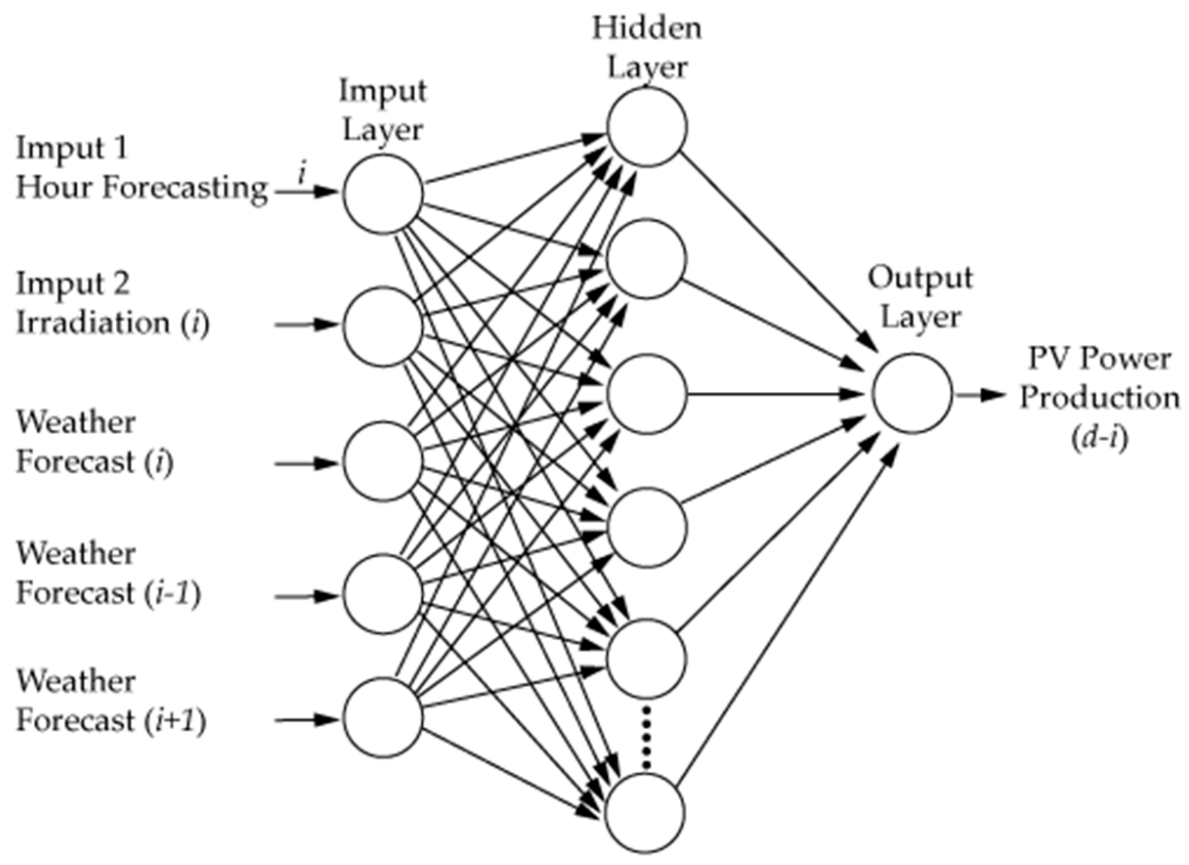
The utilized forecasting method was implemented using an ANN. The utilized ANN architecture (multi-layer perceptron) involves the need of a training, testing and validation stage; the data have to be divided into three groups to be utilized at the different stages. Moreover the correct input data have to be chosen, using only those useful for the forecasting, thus the different steps for the implementation of the forecasting method are discussed.
4.1. Forecasting Method Implementation
To forecast power production at hour h, the ANN uses as input the meteorological condition of the considered hour h, meteorological condition of hour h + 1, meteorological conditions of hour h − 1, and the hourly theoretical irradiance. The weather data for the considered day are classified according to five different general descriptions (clear sky, nearly cloudless or scattered clouds, few clouds, partly cloudy, and covered or storm). It is worth underlining that such weather information is usually available from any free weather service and downloadable, theoretical irradiance can also be easily obtained (for instance using Photovoltaic Geographical Information System—PVGis).
Although the Matlab toolbox has been used for training and to implement the ANN, thanks to its low computational weight, the forecasting method, after being trained, can be easily loaded onto a local control system present at the prosumer level and able to interact with the market.
The selected ANN typology is a multi-layer perceptron (MLP) with a supervised training algorithm; in particular, the back-propagation algorithm is used. The activation function of all of the neurons is tan-sigmoidal, while the training function is the Levenberg–Marquardt method. The implemented MLP ANN consists of one input layer, one hidden layer and one output layer. To determine the number of neurons of the hidden layer, a sensitivity analysis was conducted. The input and target data are kept constant while the number of neurons of the hidden layer are changed; with these conditions, several tests were conducted to find the configuration with the minimum mean absolute percentage error (MAPE), defined in [33] as:
where fi is the forecast value and yi is the actual value for the time period i.
The optimum number of neurons for the hidden layer that minimized the MAPE is 30. Therefore, the implemented ANN consists of the following: five input, 30 hidden layer neurons, one output neuron (hourly forecast power production).
In Figure 1, the complete ANN structure is reported for the i_th hour of the day (d) to be predicted.
4.2. Training Stage
To obtain an ANN that performs well, a training stage was conducted using a specific data set. The data were taken from the database described in Section 3; using the Matlab neural network toolbox, the data to train, validate and test the ANN were divided randomly with the sequent ratios: 0.7, 0.15 and 0.15, respectively.
The mean squared error (MSE) is used to validate the performance of the ANN in the training stage. Several tests were conducted to reach a solution with better performance.
5. Forecasting Results
In this section, the results of the implemented forecasting method are reported, considering the daily data of March 2016. It is worth emphasizing that this month was selected due to the possibility of a greater variability of weather conditions and therefore, in the authors’ opinion, more significant results.
The results are divided into three sub-sections: the first sub-section analyses the results obtained from the forecasting method for both clear and non-clear sky days; in the second sub-section, the comparison with other PV forecasting methods is evaluated; in the last sub-section, the economic considerations concerning the use of the proposed method in order to reduce the imbalance costs are reported.
5.1. Proposed Method Results
(a) PV power forecasting in the clear sky conditions
First, the prediction for clear sky days was made. The input describing the weather conditions was equal to “1”.
Figure 2 depicts the results of the PV power forecast for four days (27 to 30 March); for these days, clear sky conditions were predicted. The resulting MAPE was calculated to be 9.8%. In the hours close to sunrise and sunset, the percentage error was at a maximum; in the considered case, this was equal to 45%. The percentage error was at its minimum (less than 1%) for the hours of higher production.
Three other important parameters for evaluating the performance are the maximum absolute error, and the mean absolute error (MAE) which is defined in [33] as:
where fi is the forecast value and yi is the actual value for the time period i, and the normalized MAE (nMAE), which is the ratio between the MAE and the rated power of the PV plant. These three values are 47 kW (6.7% of rated PV Power), 18 kW and 2.6%, respectively.
It is also important to evaluate the sign of the error, that is if the error is negative (real production is higher than the forecast production) or positive (real production is less than the forecast production). This information can be used to find some possible corrections to the error and is important for the economic considerations, in particular for the estimation of ICs.
For negative errors, the MAPE was equal to 7.8%, while for positive errors, the MAPE was 13.6% (Figure 3). Figure 3 shows that the number of samples with negative discrepancy was greater than those with positive discrepancy, but the values of the negative discrepancies were smaller than the positive ones. Therefore, it is more important to reduce the positive discrepancies because their values are farther from the threshold than to reduce negative discrepancies, whose values are almost all within the threshold of 15%.
Therefore, evaluating the permanence of the percentage error below a given threshold is necessary. This threshold operates in an easier way, without incurring excessive unbalance costs due to forecast errors. The permanence of the MAPE below the threshold of 15% was evaluated: 87% of the forecast power values remained below the given threshold, but higher variances were verified at sunrise and sunset, when power production is lower and so imbalance costs are negligible. As expected for the clear sky condition, on these days, the PV power forecast accuracy was greater than 90%. This is a good value considering the practicality of the method, the limited historical data, and the orientation of the PV plant.
(b) PV power forecasting in non-clear sky conditions
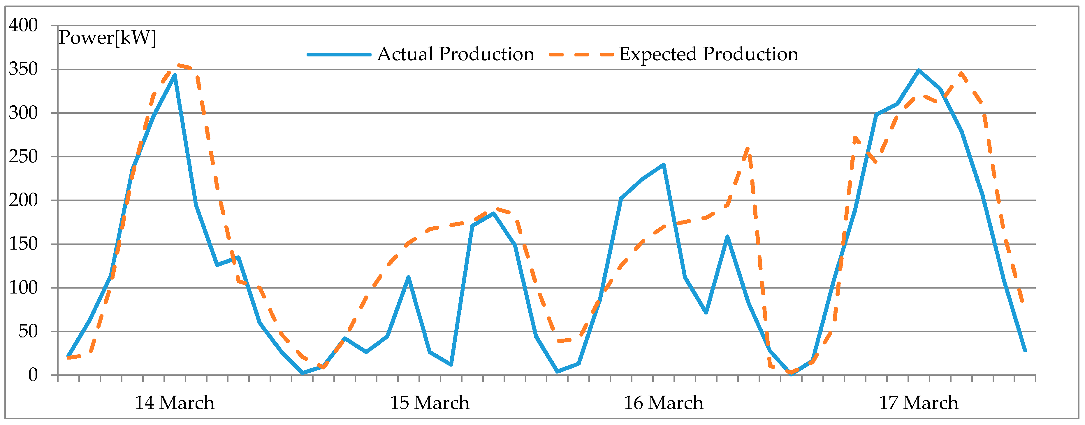
The same ANN was also trained for non-clear sky conditions. For non-clear sky conditions, the weather data for the ANN range from “2” to “5”. Compared to the forecast in the clear sky conditions, a lower accuracy was expected. To show some results, four days (14 to 17 March 2016) were considered; for these days, the expected weather conditions were variable. In Figure 4, the forecast results are shown. The calculated MAPE was 42%; in the hours close to sunrise and sunset, the maximum percentage error occurred and was equal to 169%. Similar to the clear sky forecast, the nMAE was calculated equal to 6.8%. The maximum absolute error was 180 kW, which is equal to 25.7% of the rated PV power.
The absolute error is relevant because it depends on the accuracy of the weather forecasts: an error in the weather forecast amplifies the error of the PV power forecasts. In Figure 4, it is possible to observe the error due to the discrepancy between the expected and actual PV power production. For example, on 16 March, at 4:00 pm, the expected production was higher than the real production because the expected weather condition was “partly cloudy”, while the actual weather was “rainy”. The permanence of the percentage error below the 15% threshold was evaluated: 31% of the samples remained below this threshold. The sign of the prediction errors was evaluated. The MAPE calculated for negative errors was 40%, while for positive errors, it was 60% (Figure 5).
More negative error samples exceeded the 15% thresholds than positive errors; therefore, the expected production was greater than the actual production. The high error is due to the lower reliability of the weather forecast when non-clear sky conditions are predicted; it is worth underlining that the weather reliability is given by a weather forecast website. The reliability of the weather forecast using ANN inputs was greater than 90% for clear sky conditions but less than 80% for non-clear sky conditions. As explained in [12], this weather uncertainty led to a greater error.
More negative error samples exceeded the 15% thresholds than positive errors; therefore, the expected production was greater than the actual production. The high error is due to the lower reliability of the weather forecast when non-clear sky conditions are predicted; it is worth underlining that the weather reliability is given by a weather forecast website. The reliability of the weather forecast using ANN inputs was greater than 90% for clear sky conditions but less than 80% for non-clear sky conditions. As explained in [12], this weather uncertainty led to a greater error.
5.2. Comparison with other Methods
To validate the proposed method, the results were compared with those obtained by other methods utilizing different techniques.
This comparison highlights how this method, although it is not sophisticated, can be utilized to forecast PV power production, avoiding excessive imbalances; moreover, if the forecasting methods results are comparable, it can be stated that the subsequent economic evaluations are not invalidated by the used predictive method.
In [14], power forecasts for three different locations were realized; one of these locations is Catania (South Italy), similar to the location considered in this paper. For Catania, the following results were obtained: for non-clear sky days the nMAE was about 13%, while for clear sky days it was about 4%. In [34], the obtained nMAE for non-clear sky days was between 9.12% and 12.42%, while for clear sky days was about 4.85%. Thus, the results of the proposed method in this paper are comparable with those of [14,34], which utilize elaborate techniques and input data not always available.
Below, a comparison with [12] is reported; the attention is focused on [12] because its implemented method is similar to that proposed in this paper; moreover, the comparison was been made also using graphic support. The method in [12] predicts the PV production 24 h ahead using an artificial neural network; the required inputs are past power measurements and meteorological forecasts of the solar irradiance, relative humidity and temperature at the site of the PV power plant.
The accuracy in [12] was evaluated using MAPE. This parameter was observed: for sunny days, the MAPE was 9% (from 8.29% to 10.8%), for cloudy days, the MAPE was an average of 10% (from 6.36% to 15.08%), and for rainy days, the MAPE was approximately 38% (from 24.16% to 54.44%). Comparing the MAPE calculated by the proposed method, the values are comparable, indeed, with the proposed method, for clear sky days the MAPE was 9.8%, while for non-clear sky days it was 42%.
Moreover, to compare the method implemented in [12], in Figure 6, the actual PV production was considered (line-1). Starting from actual production, an error band was obtained, utilizing the MAPE of the method [12]. Line-2 was obtained considering a constant error of 38% greater than the actual profile, while line-3 was obtained considering a constant error equal to 38%, lower than the actual profile. In this case, a cloudy day was considered. In Figure 7, the same analysis was conducted for a sunny day; a percentage error equal to 9% was considered for line-2 and line-3. After obtaining this range, the forecast production obtained using the method implemented in this paper (line-4) was evaluated to determine whether it remained within this error band. This comparison was performed for both a sunny day and a rainy day (Figure 6 and Figure 7).
6. Economic Evaluation
The forecasting model was operated and allowed to work with the considered test plant in the Italian PCE. Indeed, the model was utilized to generate the production schedule to send to the TSO. Figure 8 describes how the model operates: weather forecasts and average daily monthly radiation were downloaded and analysed to create the input vector for the ANN and the production schedule for 48 h ahead was returned. It was observed that this process employs a total time of about 30 s, which was less than that in [35]. Using the historical data, the operators carried out a consistency check; if this check was successful, the .xml file for the production schedule was uploaded, otherwise a correction was carried out. These operations were carried out every day, whereas at the end of month, the TSO calculates and invoices the producer for the imbalance costs.
The evaluation of the imbalance costs from February 2016 to October 2016 is evaluated below. Table 2 shows, in the second and third columns, the values of the gain from the sale of measured energy (SME), that represents the total income of a zero-error prediction method, and the gain from the sale of the forecast energy (SFE), both valued at the zonal price. The fourth column shows the imbalance costs (IC) invoiced by the TSO and calculated as reported in Section 2.
The fifth column represents the total earning (TE) for the producer, that is the sum of the SFE and IC, while the last column shows the real loss or gain (Δ) with respect to the SME, in fact Δ is defined as the difference between the TE and SME. To better understand the difference between IC and Δ, and the usefulness of the proposed method, the analysis is now focused on only March, because it was a particularly variable month.
In Table 3, to better understand how the imbalances costs are calculated, the imbalance and the corresponding payments are reported for a specific day (19 March 2016). Table 3 reports, from the first to the sixth columns, the hour of the day, the energy forecast by the proposed method, the real energy measured by the TSO, the imbalance value, the sign of the imbalance in the referred area (provided by the TSO), and the zonal price (day-ahead market price of the sales offers). In the seventh and eighth columns, represents the lowest price among the purchase offers accepted for secondary reserve (SR) used in the balancing market (BM) and the use of other services (OS); is equal to the highest price among the sale offers agreeing to the use of SR and the use of OS. The last two columns are the imbalance price obtained as described in Section 2 and the total imbalance cost for the examined day.
Figure 9 shows the economic comparison between the forecast profile and the production profile with no errors (i.e., the measured profile) for March 2016. The three trends shown are as follows: black line represents the profit from the sale of forecast energy, supposing that the sale price is the zonal price (), red line represents the profit from the sale of measured energy and blue line shows the imbalance payments obtained using the proposed forecast method. If the measured energy was sold at the zonal price, the total gain would be equal to 2697.09 € in March; for the forecast production, the total gain would be equal to 2512.49 €, for a total difference of 184.59 €.
The daily imbalance payments can be positive or negative, depending on the sign of the zonal aggregated imbalance, as shown in the fifth column of Table 3. In the examined case, when the imbalance payment is negative, the producer must pay a fee to the TSO, while if the imbalance payment is positive, the producer receives money from the TSO.
In the examined case, for the month of March, the imbalance payments, using the implemented PV forecasting method, are positive. Therefore, an amount of 92.73 € was received by the user from the TSO. The difference in the gain obtainable with the measured energy decreased to 91.85 €, which is a loss of 3.4% compared to a perfect dispatchable profile (zero prediction errors), with no additional costs for data used in the prediction method due to the weather forecast (which are about 60 € per month and for every user).
Sensitivity Analysis
To evaluate the relation between the ICs and other parameters, ICs for different months were considered. First, starting from the obtained imbalances (using the implemented forecasting method), they were reduced, keeping their sign unchanged. For the different error reduction thresholds, the ICs and the economic losses/gains obtained from the sale of energy were calculated (Table 4), as explained before; they were reported in relation to the total earning due to the sale of energy (Δ %).
As the table shows, if the forecast accuracy increases, an increase or a decrease of ICs may occur (however, there was a decrease of the absolute value of the same ICs); as a consequence, the SFE varied. Overall there was a general increase of the TE, this increase was not verified for all the considered months, for some months the TE decreased with the increase of forecast accuracy, as for April.
This is due to the factors related to ICs, as explained in the second paragraph, these charges depended on the zonal price and the sign of zonal aggregated imbalance.
Indeed, for the month of April it was observed that as the number of hours for which there was a positive production imbalance and a negative zonal imbalance was greater, the imbalance was evaluated positively to max ( and ). In this way, the increase of forecast accuracy would lead to an estimation of the unbalanced energy to the zonal price which is less than or equal to the maximum (, ). In Figure 10, the trend of Δ % varying the accuracy of the forecasts, for the four considered months, is shown.
It is possible to understand that there is not a preferred direction to IC reductions, so a way to operate a priori to reduce IC and increase TE does not exist. It is necessary to avoid excessive imbalances, because they would contribute heavily to an IC increase. It would be more useful for the user to understand the IC extent and how to reduce them in real-time, by knowing the electricity market results, without programming a priori any choices.
In fact, it is possible to observe that ICs depend on several factors, such as weather conditions. It is possible to analyze the ICs in relation to day type (clear/not-clear sky), calculate the ICs for the different day types, and relate them to the respective number of days. This analysis was carried out considering four months with a not negligible weather variation (Table 5).
For the clear and non-clear sky days, the TE including and not including the IC were calculated.
It is possible to observe that IC and Δ do not have a defined trend as a function of the considered day type; the particularity is that for the non-clear sky days there is greater instability in the IC calculation, as consequence a greater risk. By calculating the relationship with the energy produced in the two day types, it is possible to observe that this ratio (Δ/Prod.Energy) is greater (in absolute value) for the clear-sky days; this behavior is also observed by referring Δ to TE.
The user, knowing their production schedule and the weather forecast, should try as much as possible—especially for non-clear sky days—to follow this profile, for example by controlling storage systems or the electrical loads. A priori knowledge of the outcome of the dispatching services market would be particularly interesting.
7. Conclusions
In this paper, a feasible forecasting method for a building-integrated PV power system was described; this forecasting method utilizes as input accessible and free data. The obtained nMAE for clear sky conditions was equal to 2.6%, whereas for non-clear sky conditions it was equal to 6.8%.
This method was also compared with other methods and the comparison highlights how this method can be utilized to forecast PV power production, and that the economic evaluations are not invalidated by the utilized forecasting method. Due to its effortlessness, the proposed method is very cheap and suitable for helping prosumers to know and reduce their imbalance costs. The economic evaluations regarding the utilization of the method in the electricity market were also reported. Based on the generation data and electric market data for the months from February to October 2016, a comparison between the PV production profile with no errors (measured energy) and the forecast profile with the proposed method was reported; for instance, for March 2016, using the proposed forecasting method, the earnings were 3.4% less than a perfect dispatchable profile (zero prediction errors). The imbalance costs were limited with respect to the obtainable profit considering a dispatchable profile, with no additional costs for forecasting production. In the reported sensitivity analysis, a comparison between several forecast accuracies was carried out, it showed that although there was no preferred correlation between forecast accuracy and the imbalance charges, the ICs decreased (as modulus) with the increase in accuracy. Moreover, an analysis considering the different weather conditions was reported, it highlights how the cloudy day forecasts are undefined and present a greater variability, so the ICs (as modulus) related to the energy production are greater for cloudy days than for clear sky days, but there is no defined trend for the total losses. Therefore, for a prosumer it is useful to adopt a production forecasting method, and a tool to estimate the imbalances and the ICs and reduce them. For small user this tool has to be very cheap, so the necessity for a cheaper (accessible) and accurate forecasting method.
Acknowledgments
This work was financed by the Italian Ministry of Economic Development (MISE) and the Ministry of Education, University and Research (MIUR) through the National Operational Program for Development and Competitiveness 2007–2013, Project DOMUS PON 03PE_00050_2.
Author Contributions
N.S. and D.M. conceived and designed the experiments; P.V. performed the experiments; A.P. and A.B. analyzed the data; G.B. contributed data and analysis tools; P.V. and N.S. wrote the paper.
Conflicts of Interest
The authors declare no conflict of interest.
References
- Ackermann, T.; Andersson, G.; Söder, L. Distributed generation: A definition. Electr. Power Syst. Res. 2001, 57, 195–204. [Google Scholar] [CrossRef]
- Wang, F.; Zhen, Z.; Mi, Z.; Sun, H.; Su, S.; Yang, G. Solar irradiance feature extraction and support vector machines based weather status pattern recognition model for short-term photovoltaic power forecasting. Energy Build. 2015, 86, 427–438. [Google Scholar] [CrossRef]
- Canova, A.; Giaccone, L.; Spertino, F.; Tartaglia, M. Electrical impact of photovoltaic plant in distributed network. IEEE Trans. Ind. Appl. 2009, 45, 341–347. [Google Scholar] [CrossRef]
- Carrasco, J.M.; Franquelo, L.G.; Bialasiewicz, J.T.; Galván, E.; PortilloGuisado, R.C.; Prats, M.M.; Moreno-Alfonso, N. Power-electronic systems for the grid integration of renewable energy sources: A survey. IEEE Trans. Ind. Electron. 2006, 53, 1002–1016. [Google Scholar] [CrossRef]
- Eltawil, M.A.; Zhao, Z. Grid-connected photovoltaic power systems: Technical and potential problems—A review. Renew. Sustain. Energy Rev. 2010, 14, 112–129. [Google Scholar] [CrossRef]
- Pepermans, G.; Driesen, J.; Haeseldonckx, D.; Belmans, R.; D’haeseleer, W. Distributed generation: Definition, benefits and issues. Energy Policy 2005, 33, 787–798. [Google Scholar] [CrossRef]
- Batalla-Bejerano, J.; Trujillo-Baute, E. Impacts of intermittent renewable generation on electricity system costs. Energy Policy 2016, 94, 411–420. [Google Scholar] [CrossRef]
- Hirth, L.; Ziegenhagen, I. Balancing power and variable renewables: Three links. Renew. Sustain. Energy Rev. 2015, 50, 1035–1051. [Google Scholar] [CrossRef]
- Gianfreda, A.; Parisio, L.; Pelagatti, M. The Impact of RES in the Italian Day—Ahead and Balancing Markets. Energy J. 2016, 37. [Google Scholar] [CrossRef]
- Antonanzas, J.; Osorio, N.; Escobar, R.; Urraca, R.; Martinez-de-Pison, F.J.; Antonanzas-Torres, F. Review of photovoltaic power forecasting. Sol. Energy 2016, 136, 78–111. [Google Scholar] [CrossRef]
- Brusco, G.; Burgio, A.; Menniti, D.; Pinnarelli, A.; Sorrentino, N. Energy management system for an energy district with demand response availability. IEEE Trans. Smart Grid 2014, 5, 2385–2393. [Google Scholar] [CrossRef]
- Chen, C.; Duan, S.; Cai, T.; Liu, B. Online 24-h solar power forecasting based on weather type classification using artificial neural network. Sol. Energy 2011, 85, 2856–2870. [Google Scholar] [CrossRef]
- Yang, C.; Thatte, A.A.; Xie, L. Multitime-scale data-driven spatio-temporal forecast of photovoltaic generation. IEEE Trans. Sustain. Energy 2015, 6, 104–112. [Google Scholar] [CrossRef]
- Zhang, Y.; Beaudin, M.; Taheri, R.; Zareipour, H.; Wood, D. Day-ahead power output forecasting for small-scale solar photovoltaic electricity generators. IEEE Trans. Smart Grid 2015, 6, 2253–2262. [Google Scholar] [CrossRef]
- Kraas, B.; Schroedter-Homscheidt, M.; Madlener, R. Economic merits of a state-of-the-art concentrating solar power forecasting system for participation in the Spanish electricity market. Sol. Energy 2013, 93, 244–255. [Google Scholar] [CrossRef]
- Pelland, S.; Remund, J.; Kleissl, J.; Oozeki, T.; De Brabandere, K. Photovoltaic and Solar Forecasting: State of the Art; IEA PVPS Programme: St. Ursen, Switzerland, 2013. [Google Scholar]
- Yang, H.T.; Huang, C.M.; Huang, Y.C.; Pai, Y.S. A weather-based hybrid method for 1-day ahead hourly forecasting of PV power output. IEEE Trans. Sustain. Energy 2014, 5, 917–926. [Google Scholar] [CrossRef]
- Sharma, N.; Sharma, P.; Irwin, D.; Shenoy, P. Predicting solar generation from weather forecasts using machine learning. In Proceedings of the International Conference on Smart Grid Communications, Brussels, Belgium, 17–20 October 2011. [Google Scholar]
- Shaker, H.; Zareipour, H.; Wood, D. Estimating power generation of invisible solar sites using publicly available data. IEEE Trans. Smart Grid 2016, 7, 2456–2465. [Google Scholar] [CrossRef]
- Bizzarri, F.; Bongiorno, M.; Brambilla, A.; Gruosso, G.; Gajani, G.S. Model of photovoltaic power plants for performance analysis and production forecast. IEEE Trans. Sustain. Energy 2013, 4, 278–285. [Google Scholar] [CrossRef]
- Chow, S.K.; Lee, E.W.; Li, D.H. Short-term prediction of photovoltaic energy generation by intelligent approach. Energy Build. 2012, 55, 660–667. [Google Scholar] [CrossRef]
- Chow, C.W.; Urquhart, B.; Lave, M.; Dominguez, A.; Kleissl, J.; Shields, J.; Washom, B. Intra-hour forecasting with a total sky imager at the UC San Diego solar energy testbed. Sol. Energy 2011, 85, 2881–2893. [Google Scholar] [CrossRef]
- Dolara, A.; Leva, S.; Mussetta, M.; Ogliari, E. PV hourly day-ahead power forecasting in a micro grid context. In Proceedings of the 16th International Conference on Environment and Electrical Engineering (EEEIC), Florence, Italy, 6–8 June 2016. [Google Scholar]
- Kalogirou, S.A. Artificial neural networks in renewable energy systems applications: A review. Renew. Sustain. Energy Rev. 2001, 5, 373–401. [Google Scholar] [CrossRef]
- Belli, G.; Burgio, A.; Menniti, D.; Pinnarelli, A.; Sorrentino, N.; Vizza, P. A multiperiodal management method at user level for storage systems using artificial neural network forecasts. Trans. Environ. Electr. Eng. (TEEE) 2016, 1, 29–36. [Google Scholar] [CrossRef]
- Burgio, A.; Brusco, G.; Menniti, D.; Pinnarelli, A.; Sorrentino, N.; Vizza, P. Economic evaluation in using storage to reduce imbalance costs of renewable sources power plants. In Proceedings of the 14th International Conference on the European Energy Market (EEM), Dresden, Germany, 6–9 June 2017. [Google Scholar]
- Darby, S. The Effectiveness of Feedback on Energy Consumption. A Review for DEFRA of the Literature on Metering, Billing and Direct Displays; University of Oxford: Oxford, UK, 2006. [Google Scholar]
- Mendes, A.L.S.; de Castro, N.; Brandão, R.; Câmara, L.; Moszkowicz, M. The role of imbalance settlement mechanisms in electricity markets: A comparative analysis between UK and Brazil. In Proceedings of the 13th International Conference on the European Energy Market (EEM), Porto, Portugal, 6–9 June 2016. [Google Scholar]
- Eransus, F.J. A Bidding Strategy for Minimizing the Imbalances Costs for Renewable Generators in Spanish Power Markets (No. 2016-13); Universidad Complutense de Madrid, Facultad de Ciencias Económicas y Empresariales, Instituto Complutense de Análisis Económico: Madrid, Spain, 2016. [Google Scholar]
- Klessmann, C.; Nabe, C.; Burges, K. Pros and cons of exposing renewables to electricity market risks—A comparison of the market integration approaches in Germany, Spain, and the UK. Energy Policy 2008, 36, 3646–3661. [Google Scholar] [CrossRef]
- Campoccia, A.; Dusonchet, L.; Telaretti, E.; Zizzo, G. An analysis of feed’in tariffs for solar PV in six representative countries of the European Union. Sol. Energy 2014, 107, 530–542. [Google Scholar] [CrossRef]
- 3bMeteo. Available online: www.3bmeteo.com (accessed on 26 September 2017).
- Makridakis, S.; Hibon, M. Evaluating Accuracy (or Error) Measures; Working Paper 95/18/TM; INSEAD: Fontainebleau, France, 1995. [Google Scholar]
- Shi, J.; Lee, W.J.; Liu, Y.; Yang, Y.; Wang, P. Forecasting power output of photovoltaic systems based on weather classification and support vector machines. IEEE Trans. Ind. Appl. 2012, 48, 1064–1069. [Google Scholar] [CrossRef]
- Huang, J.; Perry, M. A semi-empirical approach using gradient boosting and k-nearest neighbors regression for GEFCom2014 probabilistic solar power forecasting. Int. J. Forecast. 2016, 32, 1081–1086. [Google Scholar] [CrossRef]
Figure 1.
Artificial neural network (ANN) structure for the photovoltaic (PV) forecasting method.

Figure 2.
Clear sky forecast results; MAPE = 9.8% (mean absolute percentage error), nMAE = 2.6% (normalized mean absolute error).
Figure 2.
Clear sky forecast results; MAPE = 9.8% (mean absolute percentage error), nMAE = 2.6% (normalized mean absolute error).
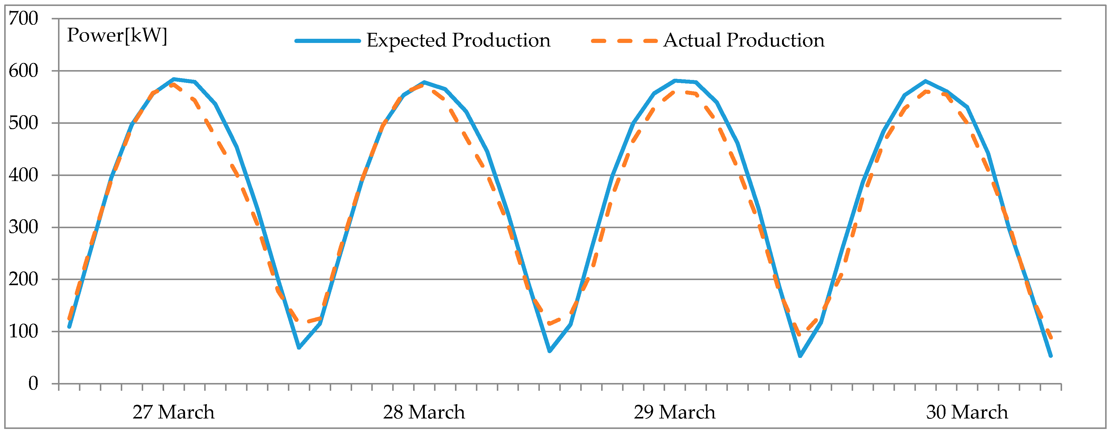
Figure 3.
Trend of the percentage error for the clear sky days forecast.
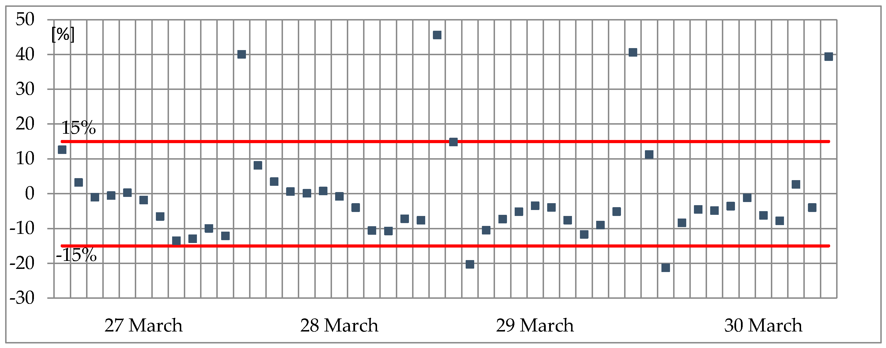
Figure 4.
Non-clear sky forecast results; MAPE = 42%, nMAE = 6.8%.

Figure 5.
Percentage error on non-clear sky days.
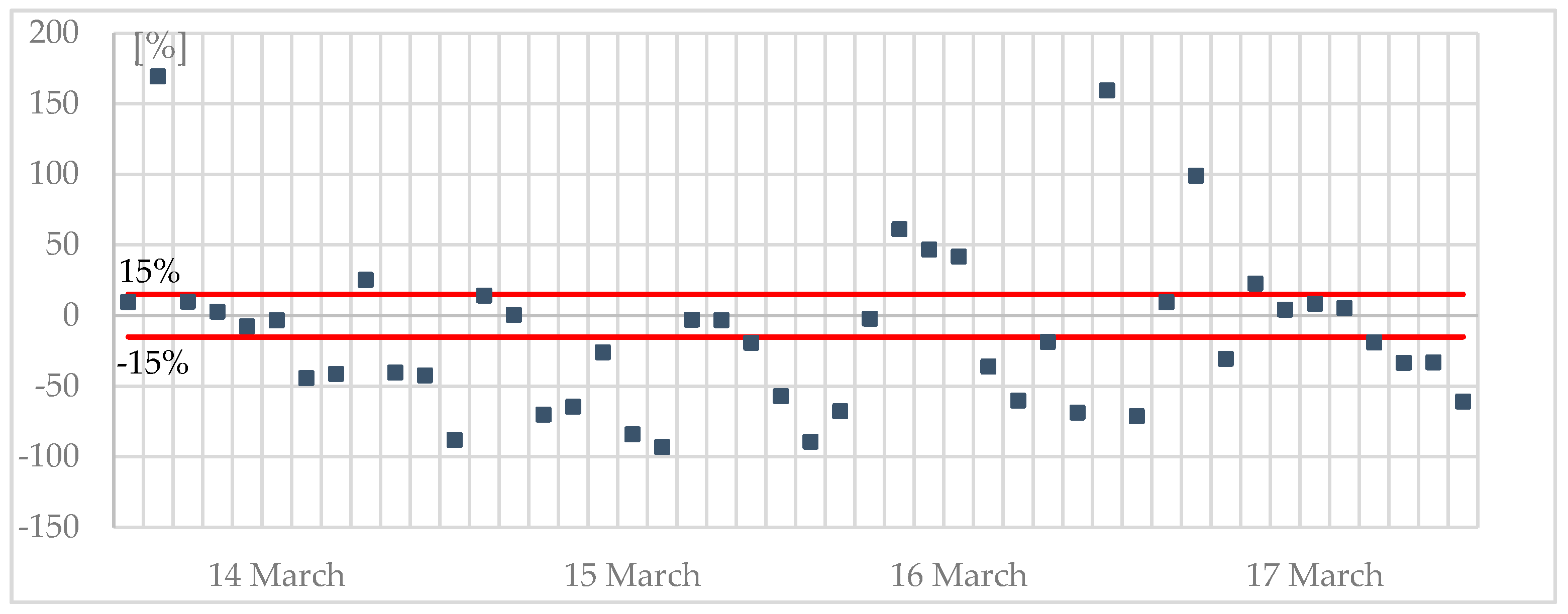
Figure 6.
Comparison with the method implemented in [14] for non-clear sky profiles.
Figure 6.
Comparison with the method implemented in [14] for non-clear sky profiles.

Figure 7.
Comparison with the method implemented in [14] for clear sky profiles.
Figure 7.
Comparison with the method implemented in [14] for clear sky profiles.
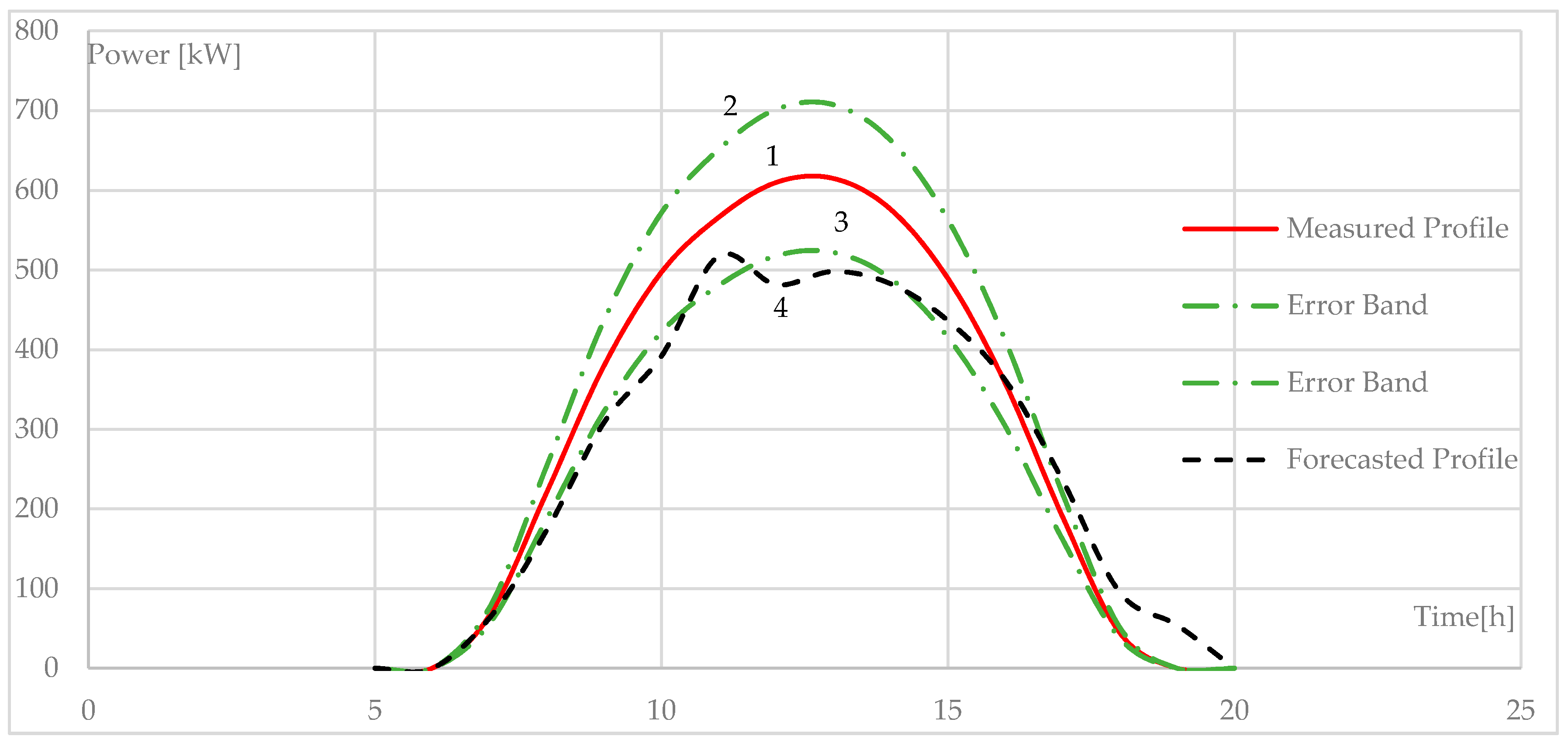
Figure 8.
Flowchart of the model operations.
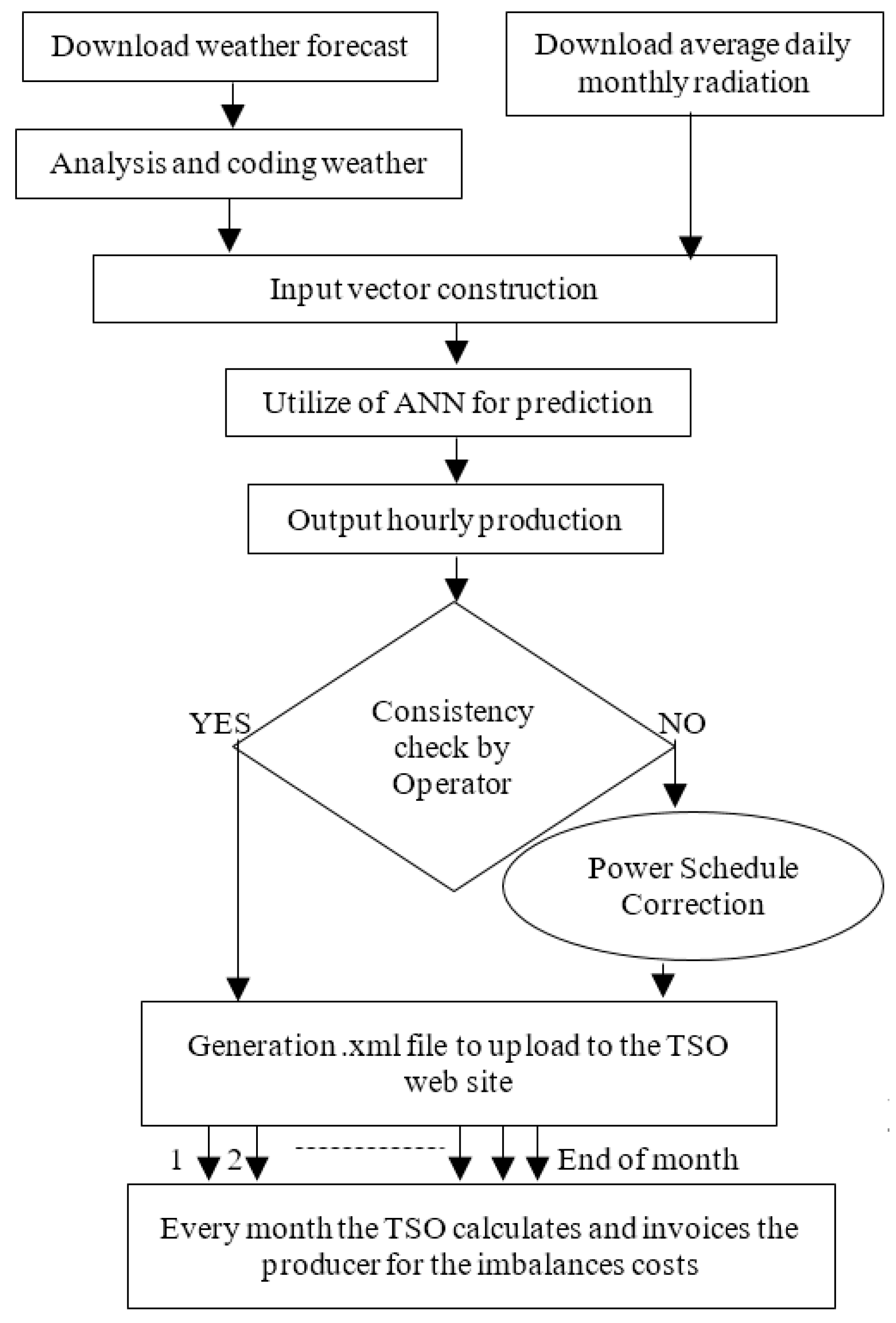
Figure 9.
Economic evaluations: comparison between the sale of measured energy and the sale of foreseen energy; imbalance costs.
Figure 9.
Economic evaluations: comparison between the sale of measured energy and the sale of foreseen energy; imbalance costs.
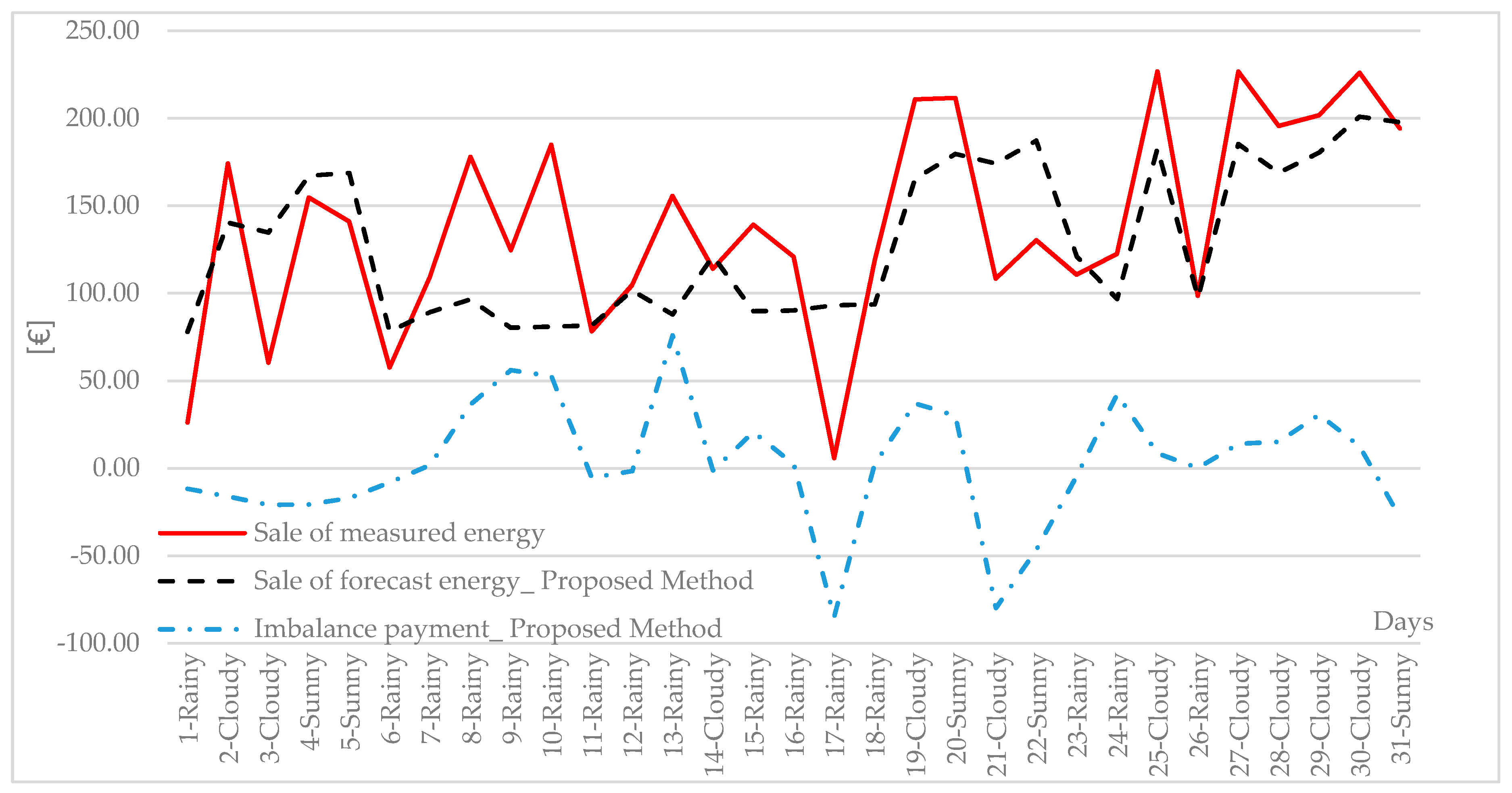
Figure 10.
Economic evaluation: losses trend with forecast error reduction.


Table 1.
Imbalance payments for unit not empowered to participate in the market.
| Imbalance Sign | < 0 | > 0 |
|---|---|---|
| > 0 | Min [, ] | Min [, ] |
| < 0 | Max [, ] | Max [, ] |
Table 2.
Economic evaluation of imbalances.
| Month | nMAE | SME [€] | SFE [€] | IC [€] | TE [€] | Δ [€] |
|---|---|---|---|---|---|---|
| February | 5.42% | 1823.38 | 2118.01 | −251.77 | 1866.24 | 42.86 |
| March | 8.45% | 2697.09 | 2512.49 | 92.73 | 2605.22 | −91.87 |
| April | 7.05% | 3556.89 | 3286.88 | 338.56 | 3625.44 | 68.55 |
| May | 11.47% | 3901.68 | 4118.03 | −326.24 | 3791.79 | −109.9 |
| June | 5.71% | 4884.96 | 4785.01 | 342.89 | 5127.90 | 242.9 |
| July | 8.85% | 6204.99 | 6065.60 | −10.43 | 6055.18 | −149.8 |
| August | 3.17% | 4554.66 | 4683.24 | −123.68 | 4559.56 | 4.9 |
| September | 9.62% | 3371.76 | 3189.03 | −5.51 | 3183.51 | −188.2 |
| October | 4.76% | 2746.38 | 2604.91 | 236.67 | 2841.59 | 95.21 |
Table 3.
Example of imbalance data and payments for a typical March day.
| Hour | Forecast Energy [kWh] | Actual Energy [kWh] | Imbalance in Area (Provided by Terna) | Zonal Price (South Area) [€/MWh] | [€/MWh] | [€/MWh] | Imbalance Price [€/MWh] | Total Imbalance Cost [€] |
|---|---|---|---|---|---|---|---|---|
| 7 | 67 | 48.16 | positive | 34.99 | 58.09 | 7.42 | 7.42 | −0.29 |
| 8 | 188 | 54.08 | positive | 29.97 | 57.52 | 4.04 | 4.04 | −0.93 |
| 9 | 291 | 150.20 | positive | 29.95 | 55.34 | 7.96 | 7.96 | −1.63 |
| 10 | 360 | 440.24 | positive | 27.00 | 57.21 | 8.65 | 8.65 | 1.22 |
| 11 | 394 | 377.5 | positive | 25.90 | 59.91 | 8.07 | 25.90 | −0.42 |
| 12 | 391 | 539.18 | positive | 25.90 | 56.03 | 6.48 | 6.48 | 1.57 |
| 13 | 261 | 325.92 | positive | 25.90 | 61.63 | 7.45 | 7.45 | 0.87 |
| 14 | 273 | 133.44 | positive | 28.00 | 64.48 | 4.91 | 4.91 | −1.19 |
| 15 | 159 | 133.15 | positive | 28.00 | 59.16 | 3.02 | 3.02 | −0.40 |
| 16 | 38 | 107.59 | positive | 32.00 | 80.77 | 2.66 | 2.66 | 0.27 |
| 17 | 39 | 2.6624 | positive | 38.25 | 165.14 | 4.43 | 4.43 | −0.27 |
Table 4.
Example of imbalance data and payments for a typical March day.
| Months | MARCH | APRIL | MAY | JUNE | ||||||||
|---|---|---|---|---|---|---|---|---|---|---|---|---|
| Error Reduction | IC [€] | SFE [€] | Δ % | IC [€] | SFE [€] | Δ % | IC [€] | SFE [€] | Δ % | IC [€] | SFE [€] | Δ % |
| 0 | 92.7 | 2512.5 | −3.40 | 338.5 | 3286.8 | 1.93 | −836.2 | 4118.0 | −15.88 | 342.8 | 4785.2 | 4.97 |
| 10% | 85.9 | 2530.9 | −2.97 | 302.5 | 3313.8 | 1.67 | −741.3 | 4096.4 | −14.01 | 305.6 | 4795.2 | 4.42 |
| 20% | 79.3 | 2549.4 | −2.53 | 266.8 | 3340.8 | 1.43 | −658.9 | 4074.7 | −12.45 | 267.6 | 4805.2 | 3.84 |
| 30% | 72.8 | 2567.8 | −2.09 | 231.2 | 3367.8 | 1.18 | −576.6 | 4053.1 | −10.89 | 229.2 | 4815.1 | 3.26 |
| 40% | 66.0 | 2586.3 | −1.66 | 195.9 | 3394.8 | 0.95 | −494.2 | 4031.5 | −9.34 | 191.0 | 4825.1 | 2.68 |
| 50% | 58.7 | 2604.7 | −1.24 | 160.2 | 3421.8 | 0.71 | −411.8 | 4009.8 | −7.78 | 157.1 | 4835.1 | 2.19 |
| 60% | 52.4 | 2623.2 | −0.79 | 122.9 | 3448.8 | 0.42 | −329.5 | 3988.2 | −6.23 | 120.8 | 4845.1 | 1.65 |
| 70% | 43.8 | 2641.7 | −0.43 | 81.8 | 3475.8 | 0.02 | −247.1 | 3966.6 | −4.67 | 89.1 | 4855.0 | 1.21 |
| 80% | 34.7 | 2660.1 | −0.08 | 43.2 | 3502.8 | −0.30 | −164.7 | 3944.9 | −3.11 | 57.4 | 4865.0 | 0.77 |
| 90% | 22.2 | 2678.6 | 0.14 | 17.3 | 3529.8 | −0.27 | −82.4 | 3923.3 | −1.56 | 20.8 | 4874.9 | 0.22 |
| 100% | 0 | 2697.1 | 0 | 0 | 3556.8 | 0 | 0 | 3901.7 | 0 | 0 | 4884.9 | 0 |
Table 5.
Example of imbalance data and payments for a typical March day.
| Months | MARCH | APRIL | MAY | JUNE | ||||
|---|---|---|---|---|---|---|---|---|
| Wheather conditions | Sunny | Cloudy | Sunny | Cloudy | Sunny | Cloudy | Sunny | Cloudy |
| TE [€] w/o IC | 1790.44 | 906.65 | 2439.94 | 1116.96 | 2822.05 | 1079.63 | 3748.8 | 1136.1 |
| TE [€] | 1741.23 | 863.99 | 2403.19 | 1222.25 | 2808.96 | 485.36 | 4024.3 | 1103.74 |
| IC [€] | 290.11 | −197.37 | 273.07 | 65.49 | 218.84 | −1042.56 | 614.3 | −271.48 |
| IC/days [€/n.days] | 17.06 | −13.16 | 15.17 | 5.46 | 12.87 | −74.47 | 30.71 | −27.15 |
| Δ [€] | 49.21 | 42.66 | 36.75 | −105.29 | 13.09 | 594.27 | −275.5 | 32.36 |
| Δ/days [€/n.days] | 2.89 | 2.84 | 1.93 | −9.57 | 0.77 | 39.62 | −16.20 | 2.16 |
| Produced energy [MWh] | 59.69 | 28.30 | 86.31 | 36.48 | 77.66 | 35.35 | 10.22 | 31.72 |
| Δ/Prod.Energy [€/kWh] | 0.82 | 1.51 | 0.43 | −2.88 | 0.17 | 16.81 | −2.69 | 1.02 |
© 2017 by the authors. Licensee MDPI, Basel, Switzerland. This article is an open access article distributed under the terms and conditions of the Creative Commons Attribution (CC BY) license (http://creativecommons.org/licenses/by/4.0/).
Share and Cite
MDPI and ACS Style
Brusco, G.; Burgio, A.; Menniti, D.; Pinnarelli, A.; Sorrentino, N.; Vizza, P. Quantification of Forecast Error Costs of Photovoltaic Prosumers in Italy. Energies 2017, 10, 1754. https://doi.org/10.3390/en10111754
AMA Style
Brusco G, Burgio A, Menniti D, Pinnarelli A, Sorrentino N, Vizza P. Quantification of Forecast Error Costs of Photovoltaic Prosumers in Italy. Energies. 2017; 10(11):1754. https://doi.org/10.3390/en10111754
Chicago/Turabian StyleBrusco, Giovanni, Alessandro Burgio, Daniele Menniti, Anna Pinnarelli, Nicola Sorrentino, and Pasquale Vizza. 2017. "Quantification of Forecast Error Costs of Photovoltaic Prosumers in Italy" Energies 10, no. 11: 1754. https://doi.org/10.3390/en10111754
Note that from the first issue of 2016, this journal uses article numbers instead of page numbers. See further details here.