Applicability of Compressive Sensing for Wireless Energy Harvesting Nodes


1
School of Electronic Engineering, Soongsil University, Seoul 06978, Korea
2
Department of Wireless Communications Engineering, Kwangwoon University, Seoul 01897, Korea
3
College of Information and Communication Engineering, Sungkyunkwan University, Suwon 16419, Gyeonggi-do, Korea
*
Author to whom correspondence should be addressed.
Energies 2017, 10(11), 1776; https://doi.org/10.3390/en10111776
Submission received: 30 September 2017
/
Revised: 24 October 2017
/
Accepted: 2 November 2017
/
Published: 3 November 2017
(This article belongs to the Special Issue Wireless Power Transfer and Energy Harvesting Technologies)
Abstract
:This paper proposes an approach toward solving an issue pertaining to measuring compressible data in large-scale energy-harvesting wireless sensor networks with channel fading. We consider a scenario in which N sensors observe hidden phenomenon values, transmit their observations using amplify-and-forward protocol over fading channels to a fusion center (FC), and the FC needs to choose a number of sensors to collect data and recover them according to the desired approximation error using the compressive sensing. In order to reduce the communication cost, sparse random matrices are exploited in the pre-processing procedure. We first investigate the sparse representation for sensors with regard to recovery accuracy. Then, we present the construction of sparse random projection matrices based on the fact that the energy consumption can vary across the energy harvesting sensor nodes. The key ingredient is the sparsity level of the random projection, which can greatly reduce the communication costs. The corresponding number of measurements is chosen according to the desired approximation error. Analysis and simulation results validate the potential of the proposed approach.
1. Introduction
A wireless sensor network (WSN) is an intelligent system with data collection, data fusion and independent transmission, which involves in many applications such as military surveillance, embedded systems, computer networks and communications. It consists of several sensors and each node is generally small in size and has a battery of limited capacity and energy. The lifetimes of WSNs thus are extremely limited by the total energy available in the batteries. Thus, using optimal techniques for energy management such as energy harvesting (EH), we can prolong the lifetime and duration of maintenance-free operation of WSNs. For instance, the energy existing in our environment from solar, wind, and thermal sources is converted into that can be used electrically. The advantages of EH-WSN solutions include high reliability, low energy needs, time savings, ecological compatibility and cost benefits [1,2,3]. In EH-WSN, each sensor node provides two functionalities: sensing, transmitting data to the fusion center (FC), and harvesting energy from ambient energy sources. The FC collects and reconstructs the observed signal by querying only a subset of sensors [4,5]. In order to reduce the energy consumption while forwarding observations to FC, we consider an innovative data gathering and reconstruction process based on three key subproblems: (i) compressive sensing (CS) based data acquisition; (ii) transmission of sparse random projection under fading for adapting random energy availability in EH systems; and (iii) CS based data reconstruction.
Data collected from wireless sensors are typically correlated, and are thus compressible in some appropriate domains. According to the CS theory, if a signal is compressible, it can be well approximated using a small number of orthogonal transform coefficients [6,7,8]. Based on the CS model, the FC receives a compressed approximation of the original signal at multiple nodes by exploiting dense random matrix, i.e., all of the EH sensors in the networks participate in forwarding observations, and the FC randomly chooses them. However, in order to avoid this situation, which consumes a large amount of energy, we first have to build a sparse random projection such that the information can be extracted from any k-sparse signal. Second, we need to design a suitable recovery algorithm to reconstruct the original signal with good accuracy for given energy neutral conditions. Therefore, it would be good for EH sensors to prolong their lifetime and for FC to query an appropriate number of random projections and to still reconstruct a good approximation. Regarding sparse random projections, a good random projection will preserve all pairwise distances with a high probability. Thus, it can be used as a reliable estimator of distances in the original space. In [9], the authors proposed a distributed compressive sensing scheme for WSNs, where the sparsity of the random projections is used consistently to reduce the computational complexity and the communication cost. They also proved that the sparse random projections are sufficient to recover a data approximation that is comparable to the optimal k-term approximation with a high probability. With the fading channel and energy-harvesting constraints, the problems regarding sparsity of random projections are studied in [10,11]. In [10], the authors only considered additive white Gaussian noise (AWGN) channels, while, in [11], the authors focused on Rayleigh fading channels and investigated sufficient conditions for guaranteeing a reliable and computationally-efficient data approximation for the sparse random projections. Due to the harvesting conditions, the sensors typically have different energy harvesting rates that lead to different available energy constraints. However, the sparsity factors in the aforementioned works have been assumed to be homogeneous for all sensors and were kept fixed for entire transmission states. Thus, they cannot be responsive to battery dynamics and channel conditions. To overcome those issues, we consider a dynamic sparsity factor that relates to the available energy constraints of wireless sensors and transmission between them, and then build a sparse random projection matrix that is stable and robust under channel fading effects and CS recovery.
The main purpose of this paper is to study sparse representation and sparse random projection for EH WSNs under fading channels. We consider a problem of data transmission in EH WSNs where multiple sensors send spatially-correlated data to a fusion center using amplify-and-forward (AF) protocol over independent Rayleigh fading channels with additive noise. Supposing that the measured data are compressible under an approximate orthogonal transform, our task is first choosing a certain number of sensors to query according to the desired approximation error by designing a sparse random projection matrix, and then exploiting the CS recovery algorithm to obtain an optimal approximation. Inspired by the work in [12] on sparse random projections for heavy-tailed data, we propose a random projection-based CS scheme where the sparsity factor is dynamic due to energy constraints. We also prove that, under the fading channel condition, our projection matrix still satisfies the restricted isometry property (RIP) for successful recovery in CS.
The organization of this paper is as follows. In Section 2, we introduce the problem of recovering a signal observed by an EH WSN under channel fading, and briefly introduce the compressive sensing. In Section 3, we present our construction on basis representations for compressible data and sparse random projection design. Section 4 proves that our sparse random matrices preserve the pairwise distance under the fading and guarantee the reconstruction accuracy subject to the energy constraints. The simulation results and conclusion are presented in Section 5 and Section 6, respectively.
Notations: We denote as a matrix whose entries are , as the matrix inverse operation, as the conjugate transpose, as the floor operation, as the number of elements in a given set T, and as the expectation and the variance operators, respectively. The norm of a vector is defined as for a positive integer p. We call a signal is a k-sparse vector if . The notation denotes the complexity operation, denotes the circularly symmetric complex Gaussian distribution with mean and covariance , and means that is distributed according to , alternatively, .
2. System Model
2.1. Problem Formulation
We consider an EH-WSN consisting of N sensors, each of which observes a single value then transmits it to the FC with the AF protocol. Note that the decode-and-forward (DF) approach can be used for sensor transmissions, where we apply digital modulation schemes to transmit the data. However, as shown in [13,14,15], for a simple distributed sensor network, the AF approach over multiple-access channel (MAC) is optimal for signal detection and estimation, as well as saving energy in relaying data. Thus, we restrict our analysis in this paper to analog transmission suitable for energy-constrained EH-WSNs, while digital modulated signals will be considered in the future work The FC collects the received signals in time slots and recovers the original signal based on this measurement as
where with ⊙ representing the Hadamard product. The matrix represents the flat fading channels between the sensors and the FC, which is a random matrix having independent and identically distributed (i.i.d.) complex circular Gaussian entries with zero-mean and unit variance, i.e., , where and . The matrix represents the random projection with energy constraints, which will be described later, is the transmitted vector, and is the additive noise where each . The real-value of Equation (1) can be written as
where
Our goal is to find a good approximation for given and . According to the CS theory, for a given upper bound of error , the FC can recover by solving the following optimization problem [6]:
However, in order to obtain recovery guarantees of a given based on Equation (4), some essential conditions for and will be considered in the next section.
2.2. Signal Reconstruction with Compressive Sensing
We define by the set of all k-sparse signals as . We say that the matrix satisfies the restricted isometry property (RIP) of order k if there exists a number such that . The best k-term approximation denoted by , can be obtained by
3. Compressive Sensing for Wireless Energy Harvesting Nodes
3.1. Motivation
In this section, we present the idea of constructing a sparse random projection and basis representation for achieving a significant speed up with little loss in accuracy recovery. First, we introduce an appropriate sparse representation basis for complex data, which takes into account data transmission cost and data recovery quality. The goal of this step is to obtain the sparse representation learned from the sensor data; thus, it has the ability to adapt the signal under fading. Second, we provide the concept of the sparse random projection, which is used for measurement matrix design. This design ensures that each sampling value represents one CS measurement guaranteeing a successful recovery, and satisfies the assumptions of energy on sensing. Finally, we verify the sparsity level and the RIP condition for the sensing matrix.
3.2. Basis Representation for Compressible Data
In practice, the signal may not be sparse, but we want to resolve it in a certain sparse basis , i.e., , where is a unitary matrix and has at most non-zero components. The matrix can be obtained either from an appropriate transform (e.g., wavelets transform, discrete Fourier transform, etc.) or from learning a dictionary to perform best based on a training set [16]. In this case, we require that satisfies the RIP and the performance will depend on . We can sort elements of the vector in the decreasing order of magnitude, where the i-th largest coefficient satisfies . Here, represents the index set of the sorted elements, where . For a rate of decay , the approximation error in -norm can be obtained by taking the k largest coefficients as
where G is a constant and [7].
3.3. Measurement Matrix: Sparse Random Projection Design
We first introduce the Johnson–Lindenstrauss (JL) lemma and its connection with the random matrix constructions of CS with regard to the stable embedding of a finite set of points under a random dimensionality-reducing projection. This lemma is stated as follows.
Lemma 1.
Let Q be a collection of finite points in . Given and , let be a random orthogonal projection from to with and
According to [17], with probability at least , for all , , the following statement holds
With respect to the JL lemma, the authors in [9,10] consider the AWGN channel, where the random projection matrix with i.i.d. entries is defined as
where is a factor that provides the probability of measurement and controls the sparsity level of . For example, if , the random matrix has no sparsity, and if , the expected number of non-zeros in each row is . Moreover, these authors proved that the are four-wise independent in rows and independent across rows, i.e.,
Note that the energy consumed for wireless transmission cannot exceed the energy available in each slot. Thus, it is reasonable to take into account both the energy constraint and the sparse random projection for reducing data transmission cost and improving data recovery quality. With regard to fading channels, Ref. [11] gave us an improvement of Equation (10), with which the projected data matrix is associated with a squared-amplitude . Each entry is
for . Given an available energy , the value of is chosen such that
It leads to , that is, the energy can be saved for the future transmission. In this paper, we define our sparse measurement matrix as , where each entry is defined by
Based on the definition of in Equation (14), the measurement vector can be expressed as in Equation (1). In the sequel, we explain the reasons for choosing this sparse random projection.
- (i)
- (ii)
- The projection given in Equation (14) selects the sensor to transmit and assigns weights to the data according to the harvested energy at the sensor. For instance, the sparsity of random projection given , can be defined aswhere is the optimal power allocation and is the available energy of node j during the i-th slot.
Therefore, we obtain
4. Proposed Distributed Algorithm and Analysis
4.1. Sparse Random Projection with Fading Channels
Suppose that we have two input vectors (alternatively, ) and the random matrix given in Equation (3). The corresponding projections of and are defined by
We also assume that under fading the channel matrix is independent of the random matrix . Thus, we have
The sparse random projection is desired to have the properties of length, distance, and inner product preservation. We need to check that those properties are still preserved under fading channel conditions. In order to check the length preservation of the sparse random matrix , we first express , where
Thus, .
For the distance preservation, we have
Similarly, we can compute the inner product as , where
Thus, the inner product is still preserved by applying since we have .
4.2. Stability and Robustness of Sparse Random Projections
By partitioning the sparse random matrix into , where each has size and ( and will be determined later), the corresponding measurement can be split into vectors . Each is defined as
We let , where and . Thus, we can perform
where and . The corresponding means, variances of , , and their covariances can be calculated as
The detailed derivations of Equations (21)–(25) are given in the Appendix A. Thus, we obtain
For any , using the Chebychev’s inequality and the fact that , we have
We have also used the fact that for any data vector , it satisfies the peak-to-total energy condition, i.e., [10]. Following the approach given in [9], the probability that an estimate lies outside the tolerable approximation interval cannot exceed , where . Setting yields , and setting gives for some constant . Finally, for , the sparse random matrix can preserve all the pairwise inner products within an approximation error with the probability of at least .
Remark 1 (Complexity Analysis).
According to CS model with a dense random matrix [6,8], it requires at least measurements for obtaining an approximation via -minimization problem in Equation (4) with probability exceeding , and the CS decoding has computational complexity . On the other hand, the sparse random projection scheme requires at least random projections and the corresponding decoding process takes , where M is the number of measurements. Since , using sparse random projection attains low decoding complexity, which makes it applicable for EH sensors, while the FC can request a little more measurements from sensors and recover the signal with a better approximation. Our proposed scheme has inherited this advantage and optimized the sparsity level, which adapts to channel conditions and energy constraints.
4.3. Sparsity Level and RIP Verification
Following the signal model in Equation (1), i.e., , the decoding process is to recover the sparse signal instead of recovering the sensor data by using Equation (4). However, we must verify that satisfies the sparse basis representation in and the matrix obeys the RIP condition to guarantee successful recovery via -minimization.
To analyze the feasibility of the measurement matrix and the sparse basis design, we have to answer the following two questions:
- (1)
- Is it reasonable to select obtained from Section 3.2 as an orthogonal basis for ?
- (2)
- For the matrix obtained from Section 3.3, does obey the RIP condition?
First, as we demonstrated in Section 3.2, the matrix is obviously an orthogonal basis in from an appropriate transformation. Otherwise, it can be an overcomplete dictionary from data learning approach, which promised to represent a wider range of signal phenomena [16].
Second, in order to show that the random variable is highly concentrated about , we can assume that the row of is independent of . Fixing , and with each row of satisfying the sub-Gaussian distribution, we prove that will satisfy the RIP with high probability, i.e.,
To do that, we prove that each part of the matrix satisfies the RIP for complex data , i.e.,
First, in order to to prove Equation (30), by letting , we have
Then, following Theorem 4.2 of [18], we obtain and . Thus,
Fixing an index set with , there are possible k-dimensional subspaces of and the probability of a k-sparse vector satisfying is given by . Here, we use the Sterling’s approximation, which states that . Thus, it leads to . Finally, we conclude that the probability of satisfying the RIP for all k-sparse vector approaches . Similarly, we obtain the same result for .
Remark 2 (trade-off between the MSE and the system delay).
There exists a trade-off between the system delay and the approximation error, which is described as follows. For an allowable mean-square error (MSE) , the achievable system delay is defined as
where ξ relates to the bounded error in Equation (6).
Thus, the total energy consumption for all sensors is . In order to minimize the total network energy consumption, should be chosen to be as large as possible, or maximizing as shown in Equation (15), which leads to the following problem.
Remark 3 (throughput maximum problem).
The optimal power allocation in Equation (15) can be obtained by solving the maximum output problem [19], which is given by
Here, and the value is a constant that depends on the hardware limitations. The above problem can be efficiently solved by using the iterative resource allocation algorithm method [19].
5. Simulation Results
We now present the results of a number of numerical simulations that illustrate the effectiveness of our approach. All simulations are performed in MATLAB R2015a (version 8.5.0.197613 (R2015a), The MathWorks Inc., Seoul, Korea) on a 3.60 GHz Intel Core i7 machine with 8 GB of RAM. We use MATLAB codes of the competing algorithms for our numerical studies. The vector was assumed to be uniformly distributed in the interval . In our work, we used the basis pursuit de-noising algorithm [20] to compute the sparse solution in Equation (4). We evaluate the performance based on the MSE, which is given by
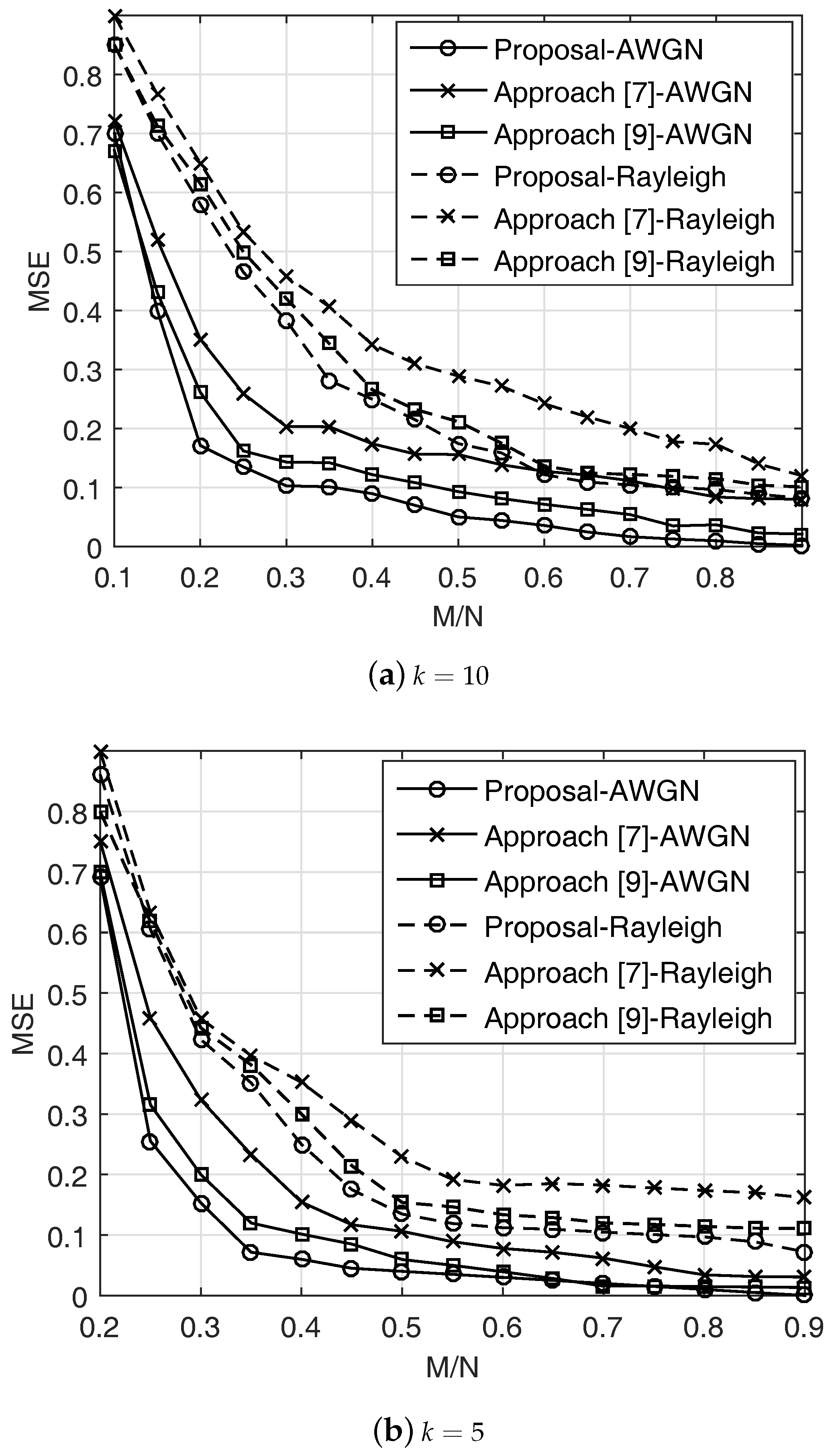
Figure 1 plots the MSE versus the compression ratio for support cardinality k and fading channels plotted for , and is uniformly distributed in the interval dB, , where dB and to guarantee a stable recovery [6]. When dB, was set at 0.25 as the conventional baseline. In order to minimize the total energy consumption, we can perform the power allocation among different transmission time slots subject to the causality of the harvested energy, which refers to the resource allocation problem with energy constraint. Note that the sparsity level in Equation (15) is still adaptive since the optimal power allocations obtained by solving the maximum output problem [1] are dynamic. The MSE values decrease as k decreases, as expected. We observed that the proposed scheme performs well compared to the conventional ones with AWGN and Rayleigh fading channels. The performance gap between those schemes is getting smaller when the ratio increases. This is because when M is large enough, the MSE may not achieve any improvements. We notice that the sparsity level of the random projection determines the amount of communication. Increasing the sparsity level yields to decrease the preprocessing cost but unfortunately increase the latency to recover a CS approximation. We will show this trade-off in the simulation results.
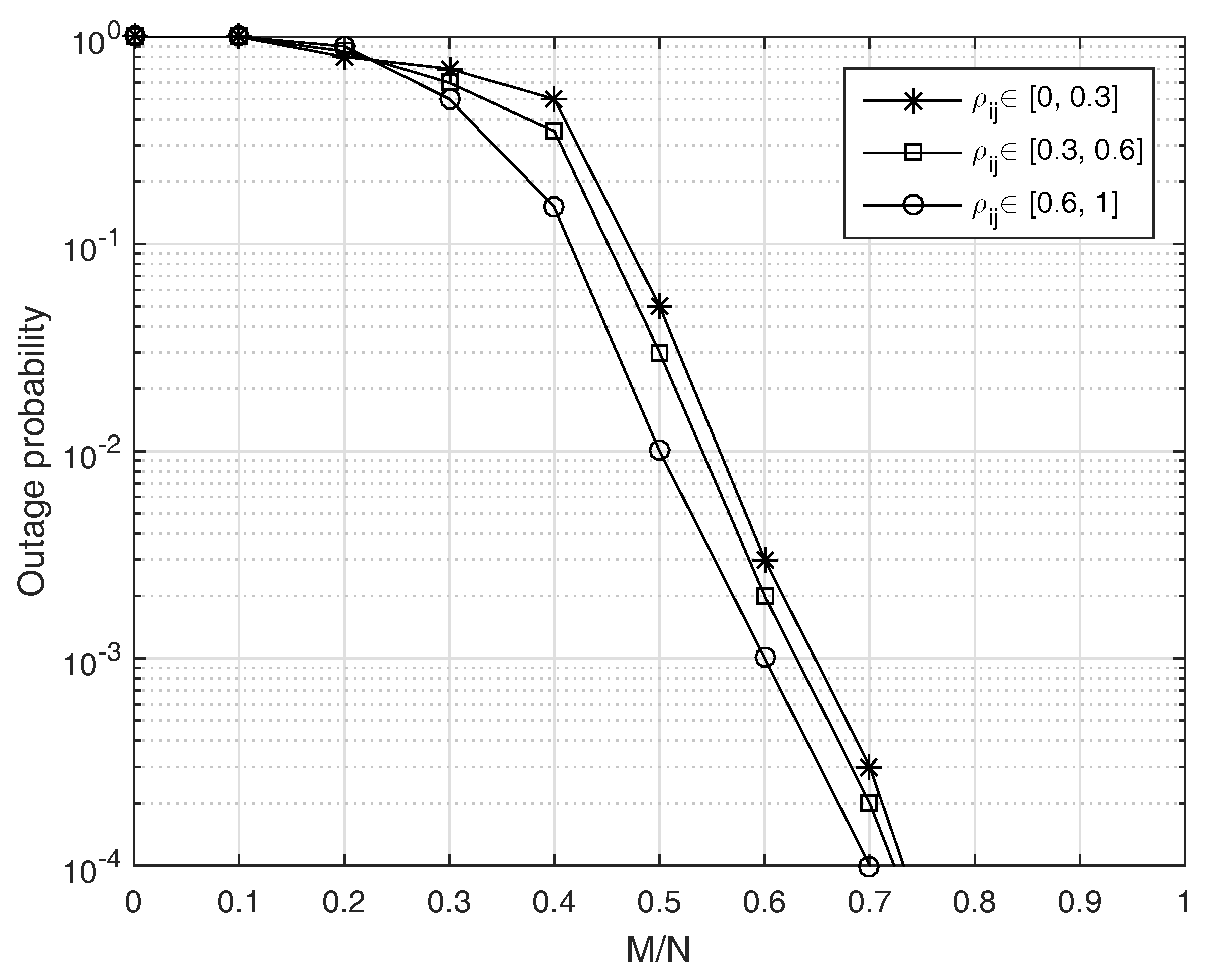
Figure 2 shows the outage probability with several intervals when and . The outage probability is defined as the probability that the matrix does not satisfy the RIP, which scales as as shown in Equation (32). For sufficiently large number M, we observe that the optimal compressed rate decreases as the sparsity level increases. This means the number of measurements M must approximately obey for effective CS recovery, while it is large enough for minimizing the outage probability. Moreover, from the result in Section 4.2, since M is proportional to , the larger value of leads to a smaller compressed ratio for a fixed N.
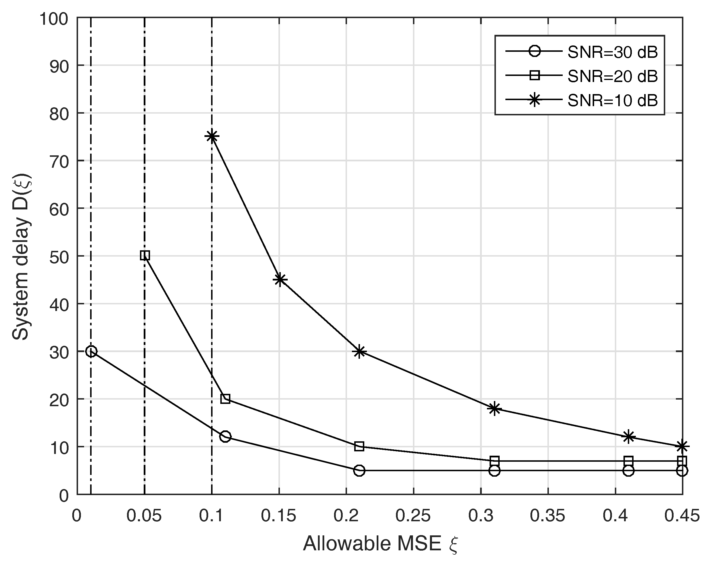
Figure 3 illustrates a trade-off between the system delay and the MSE threshold for the proposed approach as we have discussed in Remark 2 when and . We observed that the proposed scheme achieves a better trade-off when either SNR or increases as expected. This is because higher SNR means the signal is more clearly readable, the CS recovery procedure will be much easier. Moreover, for a tight MSE threshold, the procedure of choosing the estimate to minimize the expected MSE will take longer, since the best MSE scaling depends on the value of M.
Remark 4 (sparsity level option).
This scheme is developed for transformative sensing mechanisms, which can be used in conjunction with current or upcoming EH capabilities in order to enable the deployment of energy neutral EH WSNs with practical network lifetime and improve data gathering rates. However, the sparsity level in Equation (15) should be carefully chosen to maintain a good trade-off between the MSE and the system complexity. For example, when the channel condition is not good, we should select large enough (e.g., to guarantee an acceptable MSE.
6. Conclusions
In this paper, we have aimed to address the problem of recovering a sparse signal observed by a resource constrained in EH-WSNs for optimal data transmission strategy. By exploiting sparse random projections, there are significant reductions of the data measurements to be made. First, we studied a basis representation that can make the measurement matrix sufficiently sparse. The EH sensors store the sparse random projections of data, and thus the FC can estimate using compressive sensing with a sufficient number of measurements of sensors. Due to fading channels, the sparsity level can be adaptively chosen according to the available harvested energy at each EH sensor. This approach provides a better trade-off of the query latency and the desired approximation error, and also speeds up the processing time. We plan to generalize this concept in future work to incorporate sparsity of user activity and imperfect channel information as well. In addition, we would to like to emphasize that there are many ideas in the literature that would certainly enhanced our proposed scheme. We mentioned a few such possibilities as the following. First, we limited our analysis on AF protocol while different approach such as applying channel coding, and then using a modulation scheme for data transmission can be a huge open field. Second, approximation recovery for imperfect data via different norm, e.g., -norm , can be promising due to its high quality of solutions and various types of sensing matrices that can be used in the CS reconstruction algorithms. Third, it needs to further discuss how to design the sparsity parameter of the random projection matrix based on different channel fading statistics so that the number of measurements required for signal recovery at the FC is minimized. Finally, for many application of interests, we often have prior information on addition constraints, e.g., rate-energy trade-off for simultaneous information and power transfer in EH-WSNs. Thus, other sparse random projections can be provided according to those constraints.
Acknowledgments
This work was supported by the National Research Foundation of Korea (NRF) grant funded by the Korean government (MSIT) (2014R1A5A1011478).
Author Contributions
The work was realized with the collaboration of all of the authors. Thu L. N. Nguyen contributed to the main results and code implementation. Yoan Shin, Jin Young Kim, and Dong In Kim organized the work, provided the funding, supervised the research and reviewed the draft of the paper. All authors discussed the results, approved the final version, and wrote the paper.
Conflicts of Interest
The authors declare no conflict of interest.
Abbreviations
The following abbreviations are used in this manuscript:
| AWGN | Additive white Gaussian noise |
| AF | Amplify-and-forward |
| CS | Compressive sensing |
| DF | Decode-and-forward |
| EH | Energy harvesting |
| FC | Fusion center |
| i.i.d. | Independent and identically distributed |
| MAC | multiple-access channel |
| MSE | Mean-square error |
| JL | Johnson–Lindenstrauss |
| RIP | Restricted isometry property |
| SNR | Signal-to-noise ratio |
| s.t. | Subject to |
| WSN | Wireless sensor network |
Appendix A. Proofs of Equations (21)–(25)
First, the mean and the variance of are calculated as follows:
Similarly, we have
The covariance of and is obtained as
References
- Ho, C.-K.; Zhang, R. Optimal energy allocation for wireless communications with energy harvesting constraints. IEEE Trans. Signal Process. 2012, 60, 4808–4818. [Google Scholar] [CrossRef]
- Sharma, V.; Mukherji, U.; Joseph, V.; Gupta, S. Optimal energy management policies for energy harvesting sensor nodes. IEEE Trans. Wirel. Commun. 2010, 9, 1326–1336. [Google Scholar] [CrossRef]
- Lu, X.; Wang, P.; Niyato, P.; Kim, D.I.; Han, Z. Wireless networks with RF energy harvesting: A contemporary survey. IEEE Commun. Surv. Tutor. 2014, 17, 757–789. [Google Scholar] [CrossRef]
- Shaikh, F.K.; Zeadally, S. Energy harvesting in wireless sensor networks: A comprehensive review. Renew. Sustain. Energy Rev. 2016, 55, 1041–1054. [Google Scholar] [CrossRef]
- Dong, M.; Ota, K.; Liu, A. RMER: Reliable and energy-efficient data collection for large-Scale wireless sensor networks. IEEE Internet Things J. 2016, 3, 511–519. [Google Scholar] [CrossRef]
- Candès, E.J.; Romberg, J.; Tao, T. Stable signal recovery from incomplete and inaccurate measurements. Commun. Pure Appl. Math. 2006, 59, 1207–1223. [Google Scholar] [CrossRef]
- Baraniuk, R.G.; Cevher, V.; Duarte, M.F.; Hegde, C. Model-based compressive sensing. IEEE Trans. Inf. Theory 2010, 56, 1982–2001. [Google Scholar] [CrossRef]
- Davenport, M.A.; Boufounos, P.T.; Wakin, M.B.; Baraniuk, R.G. Signal processing with compressive measurements. IEEE J. Sel. Top. Signal Process. 2010, 4, 445–460. [Google Scholar] [CrossRef]
- Wang, W.; Garofalakis, M.; Ramchandran, K. Distributed sparse random projections for refinable approximation. In Proceedings of the 6th International Conference on Information Processing in Sensor Networks, Cambridge, MA, USA, 25–27 April 2007; pp. 331–339. [Google Scholar]
- Rana, R.; Hu, W.; Chou, C. Energy-aware sparse approximation technique (EAST) for rechargeable wireless sensor networks. In Proceedings of the 7th European Conference on Wireless Sensor Networks, EWSN 2010, Coimbra, Portugal, 17–19 February 2010; pp. 306–321. [Google Scholar]
- Yang, G.; Tan, V.Y.F.; Ho, C.-K.; Ting, S.H.; Guan, Y.L. Wireless compressive sensing for energy harvesting sensor nodes. IEEE Trans. Signal Process. 2013, 61, 4491–4505. [Google Scholar] [CrossRef]
- Li, P.; Hastie, T.R.; Church, K.W. Very sparse random projections. In Proceedings of the 12th ACM SIGKDD International Conference on Knowledge Discovery and Data Mining, Philadelphia, PA, USA, 20–23 August 2006; ACM: New York, NY, USA, 2006; pp. 287–296. [Google Scholar]
- Bajwa, W.U.; Haupt, J.D.; Sayeed, A.M.; Nowak, R.D. Joint source channel communication for distributed estimation in sensor networks. IEEE Trans. Inf. Theory 2007, 53, 3629–3653. [Google Scholar] [CrossRef]
- Gastpar, M. Uncoded transmission is exactly optimal for a simple Gaussian sensor network. IEEE Trans. Inf. Theory 2008, 54, 5247–5251. [Google Scholar] [CrossRef]
- Marano, S.; Matta, V.; Tong, L.; Willett, P. A likelihood-based multiple access for estimation in sensor networks. IEEE Trans. Signal Process. 2007, 55, 5155–5166. [Google Scholar] [CrossRef]
- Rubinstein, R.; Bruckstein, A.M.; Elad, M. Dictionaries for sparse representation modeling. Proc. IEEE 2010, 98, 1045–1057. [Google Scholar] [CrossRef]
- Dasgupta, S.; Gupta, A. An elementary proof of the Johnson-Lindenstrauss lemma. Random Struct. Algorithms 2003, 22, 60–65. [Google Scholar] [CrossRef]
- Davenport, M. Random Observations on Random Observations: Sparse Signal Acquisition and Processing. Ph.D. Thesis, Rice University, Houston, TX, USA, 2010. [Google Scholar]
- Ng, D.W.K.; Lo, E.S.; Schober, R. Wireless information and power transfer: Energy efficiency optimization in OFDMA systems. IEEE Trans. Wirel. Commun. 2013, 12, 6352–6370. [Google Scholar] [CrossRef]
- Berg, E.V.D.; Friedlander, M.P. Probing the Pareto frontier for basis pursuit solutions. Proc. Soc. Ind. Appl. Math. 2008, 31, 890–912. [Google Scholar]
Figure 1.
MSE versus different compressed ratios with fading channels.

Figure 2.
Outage probability with different sparsity levels.

Figure 3.
System delay for several allowable MSE thresholds.

© 2017 by the authors. Licensee MDPI, Basel, Switzerland. This article is an open access article distributed under the terms and conditions of the Creative Commons Attribution (CC BY) license (http://creativecommons.org/licenses/by/4.0/).
Share and Cite
MDPI and ACS Style
Nguyen, T.L.N.; Shin, Y.; Kim, J.Y.; Kim, D.I. Applicability of Compressive Sensing for Wireless Energy Harvesting Nodes. Energies 2017, 10, 1776. https://doi.org/10.3390/en10111776
AMA Style
Nguyen TLN, Shin Y, Kim JY, Kim DI. Applicability of Compressive Sensing for Wireless Energy Harvesting Nodes. Energies. 2017; 10(11):1776. https://doi.org/10.3390/en10111776
Chicago/Turabian StyleNguyen, Thu L. N., Yoan Shin, Jin Young Kim, and Dong In Kim. 2017. "Applicability of Compressive Sensing for Wireless Energy Harvesting Nodes" Energies 10, no. 11: 1776. https://doi.org/10.3390/en10111776
Note that from the first issue of 2016, this journal uses article numbers instead of page numbers. See further details here.