A Novel Short-Term Maintenance Strategy for Power Transmission and Transformation Equipment Based on Risk-Cost-Analysis

1
State Key Laboratory of Advanced Electromagnetic Engineering and Technology, Huazhong University of Science and Technology, 1037 Luoyu Road, Wuhan 430074, China
2
Guangzhou Power Supply Company, Ltd., Guangzhou 510000, China
*
Author to whom correspondence should be addressed.
Energies 2017, 10(11), 1865; https://doi.org/10.3390/en10111865
Submission received: 7 October 2017
/
Revised: 6 November 2017
/
Accepted: 11 November 2017
/
Published: 14 November 2017
(This article belongs to the Section F: Electrical Engineering)
Abstract
:Current studies on preventive condition-based maintenance of power transmission and transformation equipment mainly focus on mid-term or long-term maintenance, and cannot meet the requirements of short-term especially temporary maintenance. In order to solve the defects of the present preventive maintenance strategies, according to the engineering application and based on risk-cost analysis, a short-term maintenance strategy is proposed in this manuscript. For the equipment working in bad health condition, its active maintenance costs and operation risk costs are evaluated, respectively. Then the latest maintenance time is calculated in accordance with the principle that its operation risk costs are no higher than active maintenance costs. Utilizing the latest maintenance time, the best maintenance time is calculated by setting the maximum relative earnings of postponing maintenance as the target, which provides the operation staffs with comprehensive maintenance-decision support. In the end, different cases on the IEEE 24-bus system are simulated. The effectiveness and advantages of the proposed strategy are demonstrated by the simulation results.
1. Introduction
With the development of power systems, their scale is getting increasingly complicated, and the amount of power transmission and transformation equipment is getting larger as well. In order to reduce the failure probability of equipment and maintenance expenses, as well as increase the operating stability of power systems, maintenance systems have been switching from the traditional planned maintenance to condition-based maintenance [1,2], which has become the main development trend. The core of condition-based maintenance is to calculate the fault risk costs (also denoted as operation risk costs) when the equipment has been working in bad health condition for a long time and the possible expenses of active maintenance (also called active maintenance costs). In this way, reasonable maintenance time and maintenance strategy are established. There are two categories of condition-based maintenance for power transmission and transformation equipment: mid-term or long-term maintenance strategy; short-term maintenance strategy. According to the health state evaluating results, mid-term or long-term maintenance strategies offer the maintenance plan in the following half a year or later on time scale. As the health state of the equipment is time-varying and stochastic, the main problems of mid-term or long-term maintenance are that the corresponding strategies cannot apply to the practical situation once the health condition begins deteriorating. What’s more, as the mid-term or long-term maintenance strategies have a large time span, the operation risk of the equipment cannot be evaluated precisely, which has a great influence on the correctness of the strategy. Unlike mid-term and long-term maintenance, short-term maintenance makes on-line dynamic decisions by taking the operating condition of both the equipment and power system into consideration, which can compensate the deficiency of mid-term and long-term maintenance. In this way, it can improve the operation stability of both power system and power equipment, which needs to be solved urgently.
Comparing to mid-term or long-term maintenance [3,4,5,6,7], short-term maintenance takes the fluctuation of load, electricity price at different time, changes about the operation of power system, work condition of equipment and many other short-term influence factors into consideration, which can comprehensively evaluate the influence of the maintenance on the equipment itself and safety operation of power system. Considering the power transmission costs and fluctuating of load, literature [8] used the probabilistic methods to propose a maintenance strategy for transmission line. In [9,10,11], different risk evaluating indicator systems were established, which include consequence severity and economic losses. However, because of the inconsistency of measurement standard, the risk consequence cannot be evaluated precisely. In [12], by introducing interval analysis, a semi-quantitative calculation method was proposed to evaluate the risk consequence caused by the quit-operating of equipment. Because the influence factors considered in these methods are limited, the maintenance consequence on power system and equipment cannot be evaluated accurately.
Besides that, maintenance strategies have been studied by many scholars [13,14,15,16]. In [13], on the basis of the health condition prediction results, a condition-based maintenance model was established by taking the minimum value of the sum of operation risk and maintenance risk. But this model cannot make quantitative analysis uniformly. The operation state and significance of the candidate transformer were taken into consideration in [14], in which way a risk matrix was established and corresponding maintenance strategy was proposed. But a large number of operation data was needed in this strategy, which relied greatly on practical operation experience. In [15], a short-term maintenance strategy framework for transformer was brought up, by considering economic condition, operation limits and reliability of “N − 1” failure. On the basis of operation condition factors and maintenance factors, the particle swarm optimization was used in [16] to offer a maintenance plan for the transformer working in bad health condition, but these two maintenance strategies in [15,16] cannot provide the operation staff with accurate maintenance times.
As mentioned above, defects of the present condition-based maintenance strategy are as follows: firstly, mid-term or long-term maintenance strategies cannot consider the change about the operation condition of power system and the health state deterioration of equipment in the near future, which calls for the short-term maintenance strategy. Secondly, present short-term maintenance strategies mainly apply the semi-quantitative calculation methods synthesizing the severity degrees of consequence and economic losses, which lack the unified quantitative calculation methods to evaluate the risk consequence objectively and precisely. Finally, accurate maintenance time cannot be offered to operation staffs, which makes it hard in engineering application.
Aiming at solving the problems of the present condition-based maintenance strategy for power transmission and transformation equipment, this manuscript proposes a short-term maintenance strategy based on risk-cost-analysis. In order to solve the problems of unified weights and measures, the component elements of operation risk costs and active maintenance costs are brought out, following which the corresponding quantitative calculation methods are established in Section 2 and Section 3, respectively. In Section 4, for the equipment working in bad health condition, by setting the operation risk costs less than active maintenance costs as the principles, the latest maintenance time can be calculated. Besides that, on the basis of the latest maintenance time, for those equipment whose maintenance plan can be postponed, by taking the maximum relative earnings of postponing maintenance as the target, the best maintenance time can be determined. In this way, by synthesizing the latest maintenance time and best maintenance time, the risk-cost-analysis-based maintenance decision-making can be proposed, which can provide the operation staffs with multi-dimension support when scheduling short-term maintenance plan. In Section 5, IEEE 24-bus system is applied to verify the validity and correctness of the proposed maintenance strategy. Finally, conclusions are drawn in Section 6.
2. Quantitative Calculation Methods of Active Maintenance Costs
Active maintenance costs are made up of the direct costs and indirect costs. The direct costs mainly include the labor costs, material costs and transportation expenses. While the indirect costs are comprised of direct costs and indirect costs of load loss caused by quit-running of equipment. Thus, active maintenance costs can be calculated as:
where, Rre(t), Rre−1(t) and Rre−2(t) refer to the active maintenance costs, the direct costs and the indirect costs, respectively.
For Rre−1(t) in Equation (1), whose amount is usually related to time limit, number of people involved in maintenance actions and salary for each staff. Hence Rre−1(t) is mainly decided by the complexity of each maintenance action, which makes it hard to be evaluated precisely. In practical engineering application, quantity standards and guides can be used to determine the possible active maintenance expenses. Literature [17] which is promulgated by National Energy Administration of China, is widely used in field operation. This standard can provide the operation staffs with the representative budget and outage duration for different types of power equipment, which can helpfully guide the field staffs to schedule the maintenance plan. Besides, if the historical data was enough, the statistical calculation method can also be applied, shown as:
where n refers to the number of the active maintenances taken on the power equipment; Rre−1−k is the direct expense of kth active maintenance. Especially, if n = 0, which means that the equipment has never experienced active maintenance before, then Rre−1(t) of the similar equipment can be applied.
Rre−2(t) in Equation (1) are comprised of direct costs and indirect costs of load loss. From power supply enterprise point of view, direct costs of load loss can be calculated by multiplying the loss of load and the power prices during the power cut caused by the active maintenance, while indirect costs of load losses are made up of personal losses, environment loss, social loss and so on. Indirect costs are hard to be evaluated precisely for involving too many factors. Currently, literatures about maintenance strategy usually ignore these indirect costs of load loss [12,18,19], which have a great influence on the accuracy of calculating maintenance expenses. Considering that the loss of load caused by quit-running of equipment can be deemed as power operation accidents, a practical method is to calculate the compensation expenses due to power supply interruption according to certain system operation regulations. The penalty price can be referred in [20]. Hence the calculations of Rre−2(t) can be shown as:
where, Rre(t), Rre−1(t) and Rre−2(t) refer to the risk cost of active maintenance, the direct costs and the indirect costs, respectively; Rre−load−1(t) and Rre−load−2(t) denote to the direct and indirect costs of load loss; i (i = 1, 2, 3) refer to the first , second and third level load, respectively; psell−i(τ), pbuy−i(τ) and ppenalty−i(τ) refer to the electricity power selling price at different time, purchasing price and compensation price of the power supply enterprise, respectively; Tre is the duration of the active maintenance; ΔPLD−i(τ) is the i-th level load loss in terms quantified at time τ. From Equation (3), the key to calculate Rre−2(t) is to precisely evaluate the amounts of power outage, which are mainly decided by the outage duration of active maintenance and amount of load loss. The quantitative calculation methods of these two factors will be presented below.
2.1. Calculation of the Duration of Active Maintenance
Similar to Rre−1(t), the outage duration of active maintenance is decided by the complexity of the maintenance actions as well. Thus, from a practical point of view, the quantity standards in [17], or statistical calculation method can be used, shown as:
where, n refers to the number of the active maintenances taken on the power equipment; Tre−k is the repair time of the kth active maintenance. Especially, if n = 0, which means that the equipment has never experienced active maintenance before, then Tre of the similar equipment can be applied.
2.2. Calculation of the Amount of Load Loss
In current researches on quantity of load loss, Expected Energy Not Supplied (EENS) is usually used [21,22]. While, as a commonly used reliability index, EENS evaluates the load loss from a view of long time scale, which can’t precisely capture the real loss of power system when the equipment quits operating. Thus, according to the practical operation condition of power system, load loss at each moment during the outage time of active maintenance under the results of short-term load forecasting. Short-term load forecasting method such as regression analysis method, time series method, similar day method, grey forecasting method and intelligent prediction method have been studied thoroughly, which need no more introductions [23,24].
Load losses caused by active maintenance are influenced in many different aspects. When quit-operating of equipment caused by active maintenance directly leads to power interruption of the nearby load buses, the quantity of load losses is equal to the total amount of the load on the relative load buses. However, if loads on the relative load buses can be transferred to other buses, it will cause over-limit and overload on these buses. Under these circumstances, load shedding is needed. In practical operation condition of power system, load shedding caused by power transferring usually takes the significance of each load into consideration, which means that unimportant loads are cut preferentially. Thus, a load shedding model which comprehensively considers the significance of each load bus is established, whose objective function is shown as:
where, refers to the importance degree of the jth level load; Xij is the quantity of the jth level load shedding from the i-th load bus.
The proposed objective function should satisfy the following constraints:
- Power flow constraints:where, Pgi and Qgi refer to the max active power and max reactive power of the generator on bus i; Pdi and Qli refer to the active power and reactive power of the load bus i before load shedding; θij is the angular phase difference between bus i and bus j. gij and bij refer to the conductance and susceptance of the branch i and j.
- Generator output constraints:where, . and refer to the upper and lower limit of active power from generator on bus i; and refer to the upper and lower limit of reactive power from generator on bus i, respectively.
- Node voltage constraints:where, and refer to the upper and lower limit of voltage on bus i.
- Branch power transmission constraints:where, Pij, Qij, |Sijmax| refer to the active power, reactive power and transmission capacity limit of the branch i − j, respectively.
- Amount of load shedding constraints:where, means the proportion of each level load; refers to the reactive power on bus i before the load shedding.
Power flow and generator output constraints are the basic equations of power flow calculations. Node voltage and branch power transmission constraints reflect the influence of the quit-operating of equipment on other branches, which is usually evaluated by over-limit severity index. In this way, the consequence of the quit-operating of equipment can be uniformly summed up as economic indicators. By comprehensively considering all the constraints above, primal-dual interior point method can be applied to solve the established objective function. Then, in Equation (3) can be obtained.
3. Quantitative Calculation Methods of Operation Risk Costs
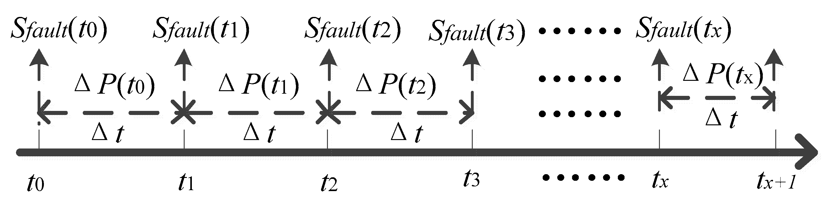
In the risk assessment of power system, risk is the product of probability and consequence. Operation risk costs refer to the expected economic losses if failure occurs, more specifically, the equipment is out of service. Different from the active maintenance costs, operation risk costs may increase with the accumulation of operation time. It not only includes the instantaneous failure risk costs at the current moment, but also contains the accumulated failure risk costs since the reference moment. Reflecting on time, the accumulation effect of operation risk costs can be shown as Figure 1. In Figure 1, time period between t0 and tx can be divided into several unit time scale, which is usually measured as 15 min. During each time unit, the accumulation operation risk costs are equal to the accumulation value of the product of accumulated fault probability and fault consequence. Its quantitative calculation equation is shown as:
where, Rfault(t) refers to the operation risk costs; means the accumulated fault probability rate in unit time; S(ti) refers to the total fault consequence at time ti.
Component elements of Sfault(ti) in Equation (11) is similar to active maintenance costs in Section 2, which are also made up of direct losses and indirect losses. It is important to note that these two losses are much larger than the losses caused by active maintenance. Thus, according to Equation (3), the calculation of operation risk costs is shown as:
where, Sfault (t) Sfault−1(t) and Sfault−2(t) refer to the total fault consequence, direct consequence and indirect consequence, respectively; Tfault refers to the duration of fault on the equipment.
From Equations (11) and (12), the key to calculate operation risk costs is to precisely evaluate the fault probability and fault consequence. As the calculation method of has been discussed in Section 2, the following parts of this Section mainly focus on the quantitative calculation methods of fault probability, direct fault consequence and duration of fault.
3.1. Calculation of Fault Probability
As an important and widely-used reliability index, fault rate of power equipment has been studied extensively [25]. In reliability analysis, fault probability of power equipment is usually evaluated from the view of equipment life [26,27]. The physical meaning of in Equation (11) is as follows: at the ti moment, the possibility of fault on equipment in the next unit time . Thus, can be described in the form of conditional probability:
where, event A notes that the fault occurs between ti and ti + , which means that the equipment life is ti and ti + ; event B notes that there is no fault before ti, which means that the equipment life is longer than ti.
Thus from the equipment life analysis view, the calculation equation of is shown as:
where, T refers to the real life of equipment; f(t) means the failure probability density function, which can be depicted by normal distribution, Weibull distribution, or exponential distribution.
From the view of engineering application, in order to describe the explicit expression, exponential distribution can be used to portray f(t), which means , where, refers to the fault rate of equipment, which is time-variable because of the change of its operation condition. Thus, it can be evaluated by its health status [28], shown as:
where, K refers to the proportionality coefficient; C is the curvature coefficient; HI means the health status evaluation index of this equipment.
K and C in Equation (15) can be obtained through inversion method; HI can be obtained from the scoring rules of power equipment health state assessment regulations.
Based on Equation (15), then Equation (14) can be calculated as:
Considering that the unit time is quite small, is very small as well, which means that in Equation (16) can be ignored. Therefore, for the equipment whose failure probability density function follows exponential distribution, its fault probability in the next unit time is approximately equal to its fault rate in unit time.
3.2. Calculation of the Failure Direct Consequence Costs and Duration of Failure
As the failure direct consequence costs and duration of failure are both primarily determined by the complexity of the maintenance after failure, then according to Equations (2) and (4) in Section 2, practical statistical computation methods are used to calculate these two elements, shown as Equations (17) and (18) below:
where, n refers to the number of faults happened on equipment; Sfault−1−k and Tfault−k refer to the maintenance expense and duration of the maintenance after the kth fault, respectively. Especially, if n = 0, which means that equipment has never experienced failure before, then Sfault−1−k and Tfault−k of the similar equipment can be applied.
4. Short-Term Maintenance Strategy Based on Risk-Cost-Analysis
Short-term maintenance plans are mainly targeted to equipment in bad health condition. The essence of the strategy is to compare the relative values between operation risk costs and the active maintenance costs when the equipment works under bad health condition. In this way, the best maintenance time can be obtained by setting the maximum economic earnings However, in the practical engineering application, as the maintenance plan is usually affected by several uncontrollable factors, such as the sufficiency of maintenance resources, there is great uncertainty about planning the maintenance actions at the best time. Thus, short-term maintenance strategy should not only provide the best maintenance time, but also the latest maintenance time, which can offer multi-dimensional maintenance decision-making support. Based on the compare between active maintenance costs and operation costs, calculations of the latest maintenance time and best maintenance time are proposed, respectively.
4.1. Calculation of the Latest Maintenance Time
When making maintenance plans at the present time t0, according to the studies above, from the viewpoint of economic cost analysis, both the fault risk cost and the active maintenance risk costs should be comprehensively compared:
- (1)
- If Rfaultl(t0) < Rre(t0), it means that the expected fault loss costs are lower than the expenses of active maintenance. In principle, this transformer doesn’t need maintenance, which means that the short-term maintenance plan on it can be postponed.
- (2)
- If Rfaultl(t0) ≥ Rre(t0), it means that the expected fault loss costs are higher than the expenses of active maintenance. So taking active maintenance is much more economical. The main reason is that the health status of this transformer is bad and its fault probability is high. Thus, for sake of reliability, this transformer needs active maintenance as soon as possible.
For the equipment whose expected operation risk costs are lower than its active maintenance costs, with the accumulation of its operation time, the fault probability keeps increasing as well. For the need of power system safety operation, the active maintenance can be postponed only when the operation risk costs Rfault(tx) are lower than the active maintenance costs Rre(tx). If Rfault(tx) exceeds Rre(tx) for the first time, the moment tx is the latest maintenance time for postponing maintenance actions, whose criteria are shown as:
where, Rfault(t0) and Rre(t0) represent the operation risk costs and maintenance costs at the moment t0, respectively; Rfault(tmax) and Rre(tmax) refer to the operation risk costs and maintenance costs at the moment tmax, respectively.
4.2. Calculation of the Best Maintenance Time
A feasible region of the maintenance time is provided to the operating staffs by calculating the latest maintenance time. In this feasible region, the maintenance expenses can be reduced by reasonably arrange the maintenance plans according to the actual load level.
It is worth noting that: on the one hand, postponing the maintenance plans when the load level is low can reduce the expenses; on the other hand, the operation risks are also increasing with the accumulation of operation time. Thus, in order to obtain the optimum economic benefits, a balance of these two risk costs should be made to determine the best maintenance time.
Assuming that the maintenance plan is postponed from t0 to tx, the reduction of active maintenance expenses is calculated as:
Correspondingly, during the period from t0 to tx, the extra operation costs is calculated as:
The difference of and is the relative earnings of postponing maintenance plan , shown as:
If SY(tx) < 0, the decrease of active maintenance costs can’t make up the increase of operation risk costs, which means that it is not economic to postpone the maintenance plan from the current moment t0 to the future moment tx.
On the other hand, if SY(tx) > 0, the decrease of active maintenance costs is higher than the increase of operation risk costs, which means that it is worth postponing the maintenance plan from t0 to tx.
According to the analysis above, in the feasible region of maintenance time, the most economical moment of postponed maintenance is the moment whose SY(tx) is the biggest. In other words, in the view of economy, based on the latest maintenance time deducted from Equation (19), the objective function and constraints of the best maintenance time are presented in Equations (23) and (24), respectively:
where, Equation (23) is the objective function to calculate the best maintenance time; Equation (24) is the time constraint.
4.3. Implementation Procedure of the Short-Term Maintenance Strategy Based on Risk-Cost-Analysis
In accordance with the previous studies, implementation procedure of the short-term maintenance strategy based on risk-cost-analysis is shown as Figure 2.
According to Figure 2, the basic steps are as follows:
- Step 1.
- Obtain the health status of the candidate power transformer: if it is in good condition, it can keep on operating; otherwise, calculate the operation risk costs Rfault(t0) and active maintenance costs Rre(t0) at the current moment according to Equations (1) and (11), respectively.
- Step 2.
- Compare Rfault(t0) and Rre(t0): if Rfault(t0) > Rre(t0), then maintenance should be taken immediately; otherwise, then the maintenance plan can be postponed.
- Step 3.
- For the candidate power transformer whose Rfault(t0) is lower than its Rre(t0), calculate its operation risk costs and active risk costs in a future time, and deduce the latest maintenance time according to Equation (19).
- Step 4.
- Based on the latest maintenance time, in accordance with Equations (20)–(24), the best maintenance time can be derived.
5. Case Study
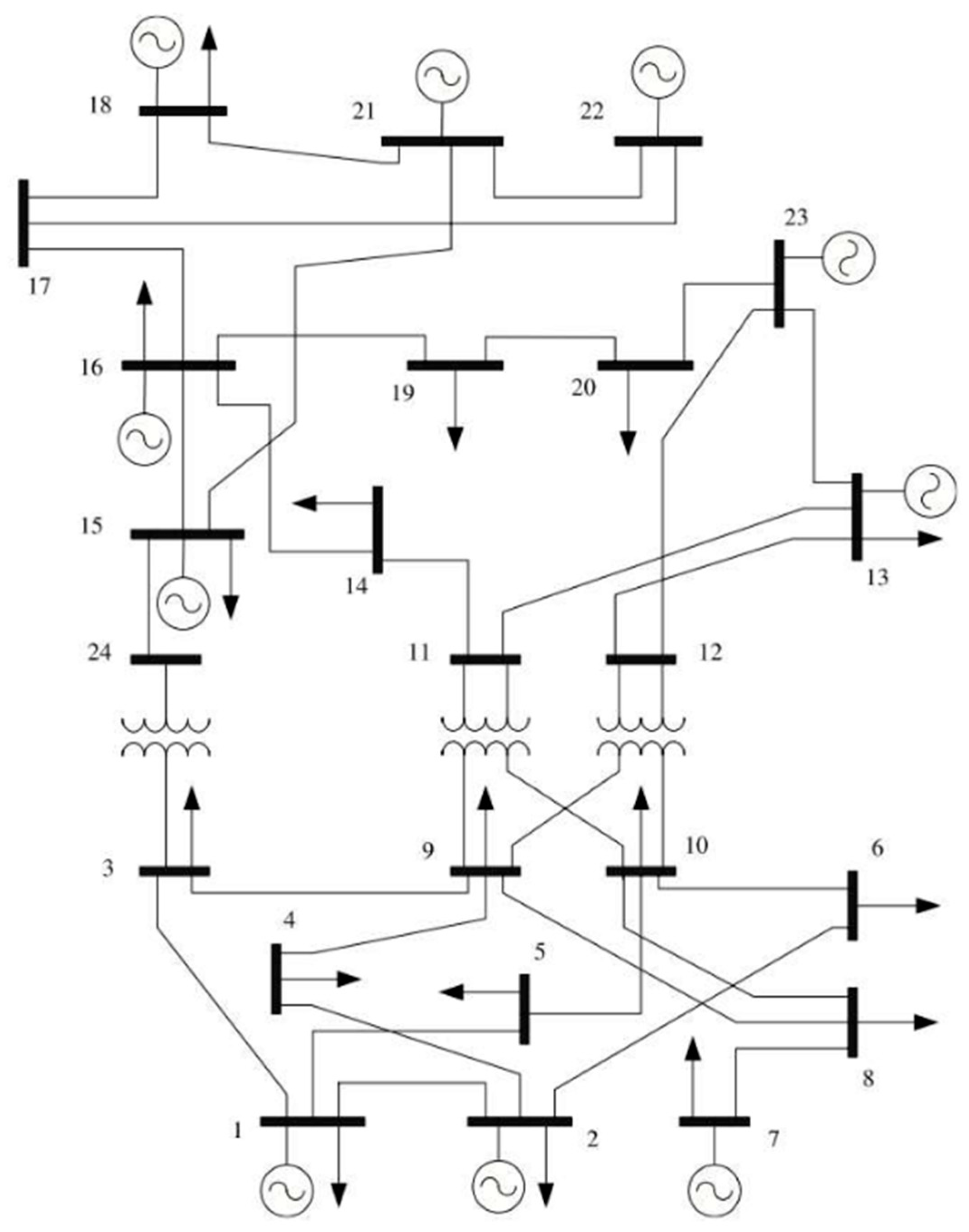
The IEEE 24-bus system [27] is employed to verify the rationality and validity of the proposed short-term maintenance strategy based on risk-cost-analysis, whose structure diagram is shown as below. The simulations are programmed based on Matpower 5.0 in Matlab (MathWorks, Natick, MA, USA), and the tests are fulfilled on a laptop with an Intel Core i5-4200 CPU at 3.4-GHz and equipped with 4 GB memory (Intel, Santa Clara, CA, USA).
In Figure 3, the transformer between the bus 3 and bus 24 is assumed in bad condition, which needs a short-term maintenance. The direct costs are as follows: Rre−1(t) = 17,761.82 ¥, Rfault−1(t) = 138,579.11 ¥ [17]. The outage duration parameters are as follows: Tre = 8 h, Tfault = 12 h [17]. The unit time is 15 min, and the fault probability .
All the load buses take the uniformly same proportions of each level load: first level load is 20%; second level load is 30%; third level load is 50%. The importance degrees of different load are as follows: , and . The electric power price data are as shown in Table 1.
The loads of the simulation system change from time to time. If the health status of the candidate transformer alarms at different time, both its operation risk costs and active maintenance costs vary a lot. Thus, the corresponding short-term maintenance strategy based on risk-cost-analysis is different. In Table 1, there are three different periods in each day. Considering the load level is usually very low at 24:00 and heavy at 19:00, these two typical situations are simulated to testify the proposed short-term strategy.
5.1. The Current Moment Is 24:00
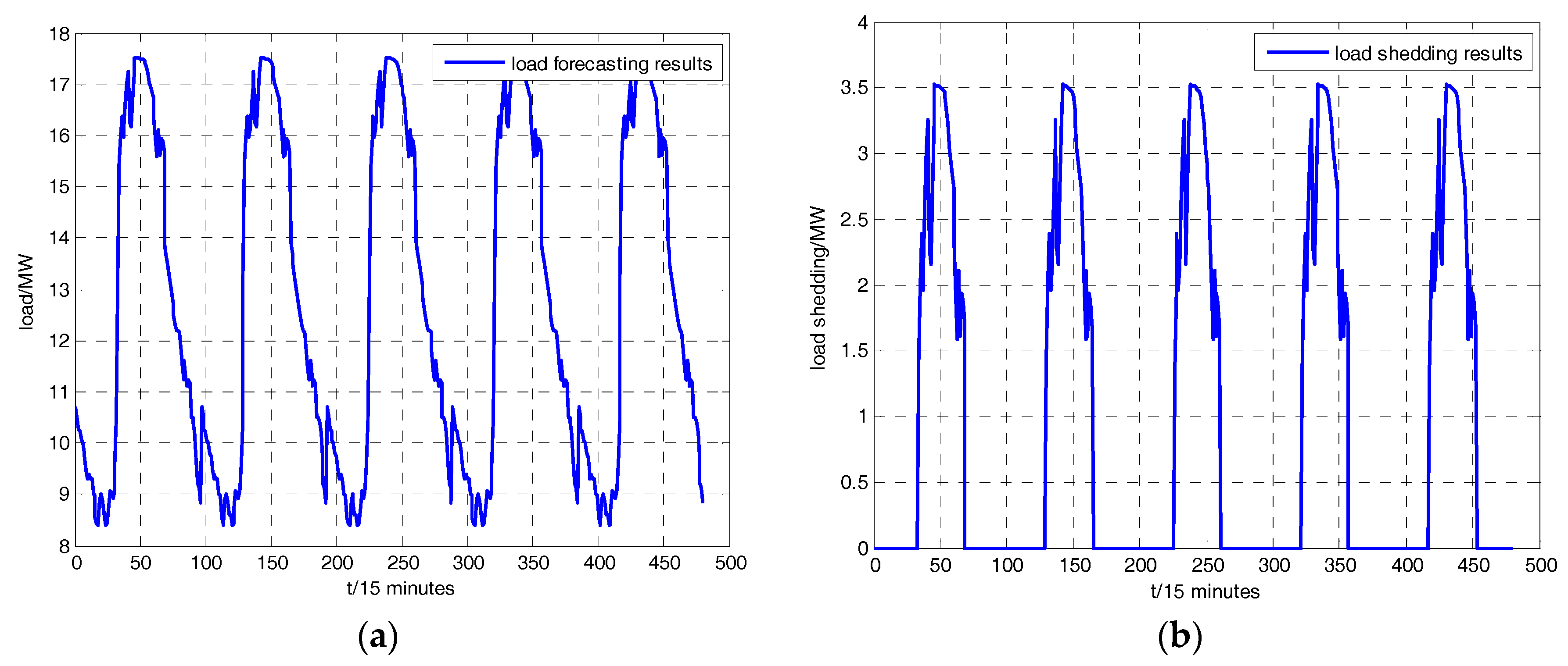
According to the load shedding model established in Section 2, when the candidate transformer between the bus 3 and bus 24 quits operating, loads at bus 17 need to be reduced. In the following 3 days, the load level of bus 17, the quantity of load shedding at bus 17 and the change trend of the risk costs of the candidate transformer are portrayed in Figure 4 and Figure 5.
From Figure 4, when the candidate equipment quits operating caused by active maintenance or failure, its quantity of load loss is changed with the actual load level of bus 17, which means that the indirect losses are fluctuating. Besides that, it can also be concluded from the two risk cost curves in Figure 5 that as the direct losses are smaller than indirect losses, the variation trends of maintenance costs are similar to the quantity of load shedding; because of the accumulation effect, the operation risk costs are increasing during the outage period caused by failure. At the current moment 24:00, since Rfault(t0) > Rre(t0), then the maintenance schedule can be postponed. When t = 56, in other words—14 h later (56 × 15 min = 840 min = 14 h), its active operation risk costs reaches its active maintenance costs for the first time. Thus, according to Equation (19), its latest maintenance time is 14 h later from the current moment. Based on the maintenance time, in accordance with Equations (20)–(24), its relative earnings of postponing maintenance plan SY(tx) is obtained, shown as Figure 6.
In Figure 6, in the next 14 h, the maximum value of SY(tx) is 0, whose time is the current moment t = 0. Thus, according to former analysis, the best maintenance time is the current moment. From the above analysis, when the health status of the candidate transformer begins deteriorating at 24:00, taking both the economy and reliability into consideration, the maintenance strategy based on the risk-cost-analysis is shown as follows: the latest maintenance time is 14 h from the current moment, in other words—14:00 next afternoon; because of the relative earnings are always below 0 except t = 0, the best maintenance time is the current moment; if there are no other requirements, operating staffs should schedule the maintenance plan at the current moment.
5.2. The Current Moment Is 19:00
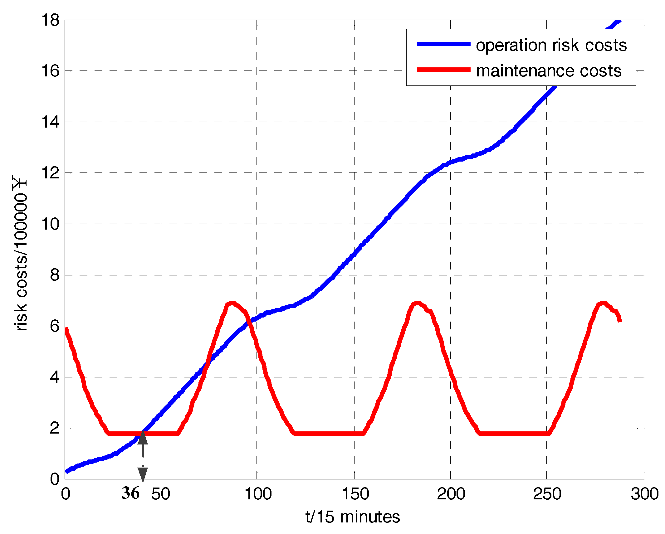
Similar to the simulation in Section 4.1, if the current moment is 19:00, when the candidate transformer between bus 3 and bus 24 quits operating, loads at bus 17 needs to be reduced. The simulation results are depicted in Figure 7 and Figure 8. Comparing Figure 8 and Figure 5, the change trends of each curve are quite similar. Since the current moment is 19:00, which belongs to the peak period, then the load level, load shedding, Rfault(t0) and Rre(t0) in Figure 8 are all higher than those in Figure 5. Moreover, as Rfault(t0) is less than Rre(t0) in Figure 8, thus the maintenance schedule can be postponed. When t = 36, in other words—9 h later (36 × 15 min = 540 min = 9 h), its active operation risk costs reaches its active maintenance costs for the first time. Thus, according to Equation (19), its latest maintenance time is 9 h later from the current moment. Based on the maintenance time, in accordance with Equations (20)–(24), its relative earnings of postponing maintenance plan SY(tx) is obtained, shown as Figure 9.
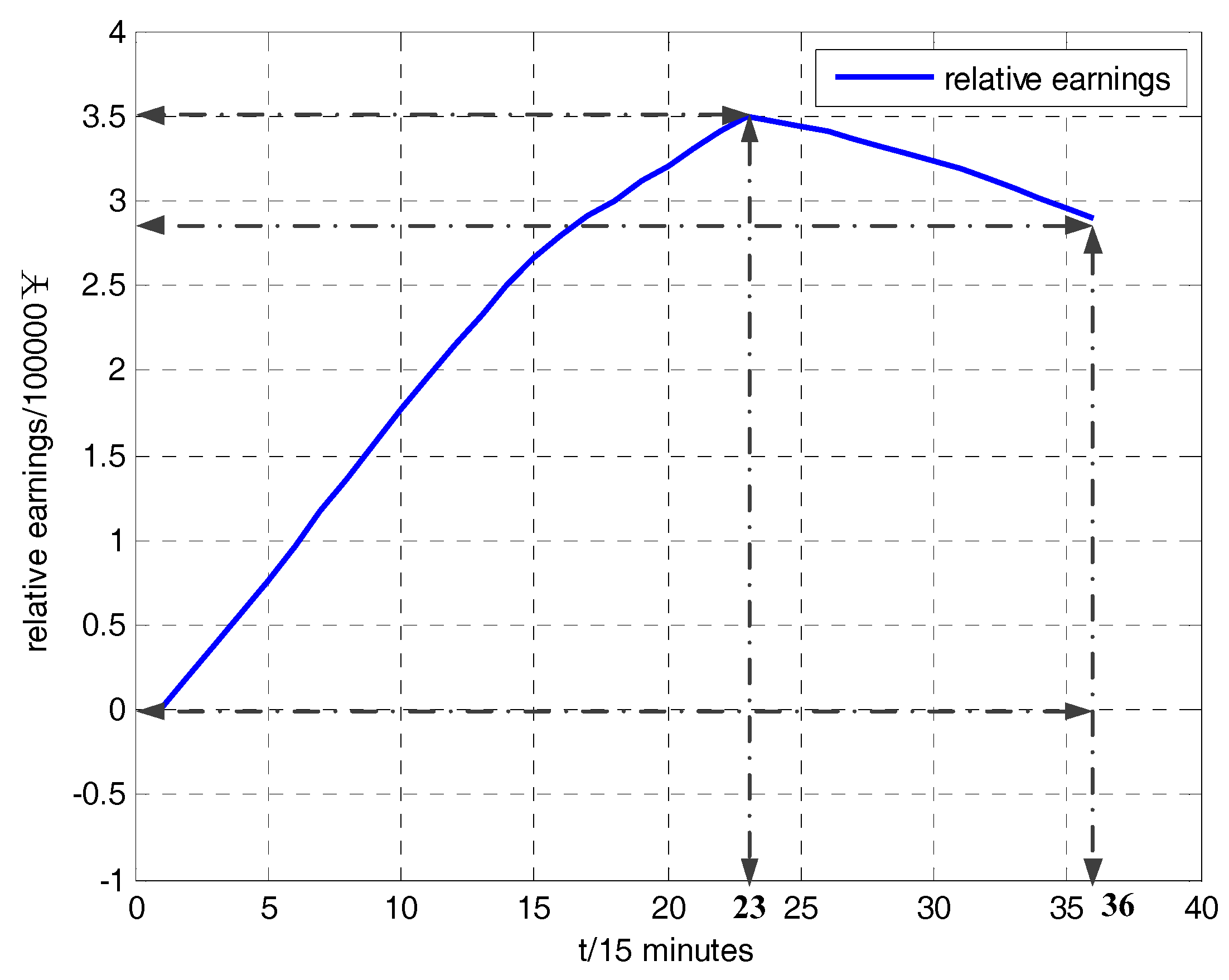
In Figure 9, in the next 9 h, the relative earnings of postponing maintenance schedule is always bigger than 0, which means that it is beneficial by postponing the maintenance schedule in this period. From the economic cost view, planning maintenance actions in this period can reduce the maintenance expenses. When t = 23, in other words—5.75 h later (23 × 15 min = 345 min = 5.75 h), it relative earnings SY(tx) reaches its maximum value, which is about 350,000 ¥. This maximum relative earnings show that, comparing to performing the maintenance at the current moment, scheduling the maintenance plan in 5.75 h later can save 350,000 ¥.
From the above analysis, when the health status of the candidate transformer begins deteriorating at 19:00, the short-term maintenance strategy based on risk-cost-analysis is shown as follows: the latest maintenance time is 9 h later, i.e., 4:00 in the next morning; the best maintenance time is 5.75 h later, which is 00:45 in the next morning; if there are no other requirements, operating staffs should schedule the active maintenance at 00:45 in the next morning.
6. Conclusions
The present condition-based maintenance strategies of power transmission and transformation equipment mainly focus on the long-term maintenance, which cannot meet the requirements of short-term especially temporary maintenance. Thus, a novel short-term maintenance strategy based on risk-cost-analysis is proposed in this manuscript, which can effectively solve the existing problems of long-term maintenance. From our theoretical studies and simulation results the following conclusions may be drawn:
- (1)
- Component elements of operation risk costs and active maintenance costs are studied, which both are made up of direct risk costs and indirect risk costs. From the view of better engineering application, economic quantitative calculation methods of these elements are proposed, which can solve the problems of unified weights and measures.
- (2)
- For those equipment whose operation status continues deteriorating, from a better engineering application perspective, based on risk-cost-analysis, calculation methods of the latest maintenance time and best maintenance time are proposed, which can offer operation staffs with accurate and multi-dimensional decision-making support when scheduling the maintenance.
- (3)
- Based on IEEE-24-bus system, two typical cases are studied: when the health status of the equipment alerts at the peak load period, its longest time of postponing maintenance plan is shorter than the equipment whose health status alerts at the valley load period; the maintenance plans should always be scheduled at low load periods by comprehensively considering economy and safety. These simulation results testify the correctness and validity of the proposed strategy.
Acknowledgments
This research is supported by the National High Technology Research and Development of China (863 Program) (No. 2015AA050201).
Author Contributions
Hang Yang, Zhe Zhang and Xianggen Yin conceived and designed the experiments; Hang Yang performed the experiments; Zhe Zhang and Xianggen Yin contributed materials and analysis tools; Hang Yang wrote the paper; Jiexiang Han analyzed the data and revised the paper; Yong Wang and Guoyan Chen provided technical support.
Conflicts of Interest
The authors declare no conflict of interest.
References
- Xu, J.; Wang, J.; Gao, F.; Shu, H. A survey of condition based maintenance technology for electric power equipment. Power Syst. Technol. 2000, 8, 48–52. [Google Scholar]
- Yang, S.K. A condition-based preventive maintenance arrangement for thermal power plants. Electr. Power Syst. Res. 2004, 1, 49–62. [Google Scholar] [CrossRef]
- Pourahmadi, F.; Fotuhi-Firuzabad, M.; Dehghanian, P. Application of game theory in reliability-centered maintenance of electric power systems. IEEE Trans. Ind. Appl. 2016, 53, 936–946. [Google Scholar] [CrossRef]
- Campelo, F.; Batista, L.S.; Takahashi, R.H.C.; Diniz, H.E.P.; Carrano, E.G. Multi-criteria transformer assest management with maintenance and planning perspective. IET Gener. Transm. Distrib. 2016, 10, 2087–2097. [Google Scholar] [CrossRef]
- Wang, H.; Lin, D.; Qiu, J.; Ao, L.; Du, Z.; He, B. Research on multi-objective group decision-making in condition-based maintenance for transmission and transformation equipment based on D-S evidence theory. IEEE Trans. Smart Grid 2015, 2, 1035–1045. [Google Scholar] [CrossRef]
- Wang, H.; Huang, H.; Li, Y.; Yang, Y. Condition-based maintenance with scheduling threshold and maintenance threshold. IEEE Trans. Reliab. 2016, 65, 513–524. [Google Scholar] [CrossRef]
- Koksal, A.; Ozdemir, A. Improved transformer maintenance plan for reliability centered asset management of power transmission system. IET Gener. Transm. Distrib. 2016, 10, 1976–1983. [Google Scholar] [CrossRef]
- Marwali, M.K.C.; Shahidehpour, S.M. Short-term transmission line maintenance scheduling in a deregulated system using a probabilistic appraoch. IEEE Trans. Power Syst. 2002, 3, 1117–1124. [Google Scholar]
- Ni, M.; Mccalley, J.D.; Vijay, V.; Tayyib, T. Online risk based security assessment. IEEE Trans. Power Syst. 2003, 18, 258–265. [Google Scholar] [CrossRef]
- Abu-Elanien, A.E.B.; Salama, A.M.M.; Ibrahim, M. Calculation of a health index for oil-immersed transformer rated under 69 kV using fuzzy logic. IEEE Trans. Power Deliv. 2012, 27, 2029–2036. [Google Scholar] [CrossRef]
- Hu, W.; Yu, T.; Wu, W. A comprehensive power grid risk assessment method based on cloud prediction model. Power Syst. Prot. Contr. 2015, 5, 35–42. [Google Scholar]
- Zhao, M.; Lu, Z.; Wu, L.; Yu, S. Risk assessment based maintenance technology for electric transmission equipment. Autom. Electr. Power Syst. 2009, 19, 30–35. [Google Scholar]
- Li, M.; Han, X.; Yang, M.; Guo, Z. Basic concepts and theoretical study of condition-based maintenance for power transmission system. Proc. CSEE 2011, 34, 43–52. [Google Scholar]
- Abiri-Jahromi, A.; Parvania, M.; Bouffard, F.; Fotuhi-Firuzabad, M. A two-stage framework for power transformer asset maintenance management—Part I: Mdels and formulations. IEEE Trans. Power Syst. 2013, 2, 1395–1403. [Google Scholar] [CrossRef]
- Abiri-Jahromi, A.; Parvania, M.; Bouffard, F.; Fotuhi-Firuzabad, M. A two-stage framework for power transformer asset maintenance management—Part II: Validation results. IEEE Trans. Power Syst. 2013, 2, 1404–1414. [Google Scholar] [CrossRef]
- Liao, R.; Yang, L.; Zheng, H.; Ma, Z. Reviews on oil-paper insulation thermal aging in power transformers. Trans. China Electrotech. Soc. 2012, 5, 1–12. [Google Scholar]
- Guo, W.; Dong, S.; Yu, M. Budget Norms of Power System Maintenance Engineering Part I: Electricity Engineering; China Electric Power Press: Beijing, China, 2015. [Google Scholar]
- Marhs, Z. Reliability centered maintenance strategy for high-voltage-networks. In Proceedings of the 2004 International Conference on Probabilistic Methods Applied to Power System, Ames, IA, USA, 12–16 September 2004; pp. 332–337. [Google Scholar]
- Yu, J.; Zhao, H. Maintenance plan based on RCM. In Proceedings of the IEEE IPES Transmission and Distribution Conference, Dalian, China, 15–17 August 2005; pp. 1–4. [Google Scholar]
- China State Council. Regulations on Electric Power Supply and Use; China Electric Power Press: Beijing, China, 2015. [Google Scholar]
- Zhao, Y.; Zhou, J.; Liu, Y. Analysis on optimal load shedding model in reliability evaluation of composite generation and transmission system. Power Syst. Technol. 2004, 10, 34–37. [Google Scholar]
- Shandilya, A.; Gupta, H.; Sharma, J. Method for generation rescheduling and load shedding to alleviate line overloads using local optimization. IEEE Proc. C Gener. Transm. Distrib. 1993, 5, 337–342. [Google Scholar] [CrossRef]
- Liu, N.; Zhang, Q.; Liu, H. On-line short-term load forecasting based on ELE with Kernel algorithm in micro-grid environment. Trans. China Electrotech. Soc. 2015, 8, 218–224. [Google Scholar]
- Gao, C.; Li, Q.; Su, W.; Li, Y. Temperature correction model research considering temperature cumulative effect in short-term load forecasting. Trans. China Electrotech. Soc. 2015, 4, 242–248. [Google Scholar]
- Li, W. Risk Assessment of Power Systems: Models, Methods, and Applications, 2nd ed.; John Willy & Sons: Hoboken, NJ, USA, 2014. [Google Scholar]
- Ning, L.; Wu, W.; Zhang, B. Analysi of a time-varying power component outage model for operational risk assessment. Autom. Electr. Power Syst. 2009, 16, 7–12. [Google Scholar]
- Subcommittee, P.M. IEEE reliability test system. IEEE Trans. Power Appar. Syst. 1979, 6, 2047–2054. [Google Scholar] [CrossRef]
- Pan, L.; Zhang, Y.; Yu, G.; Du, C. Prediction of electrical equipment failure rate for condition-based maintenance decision-making. Electr. Power Autom. Equip. 2010, 2, 91–94. [Google Scholar]
Figure 1.
Diagram of the accumulation effect on operation risk costs.

Figure 2.
The flow diagram of the short-term maintenance strategy based on risk-cost-analysis.
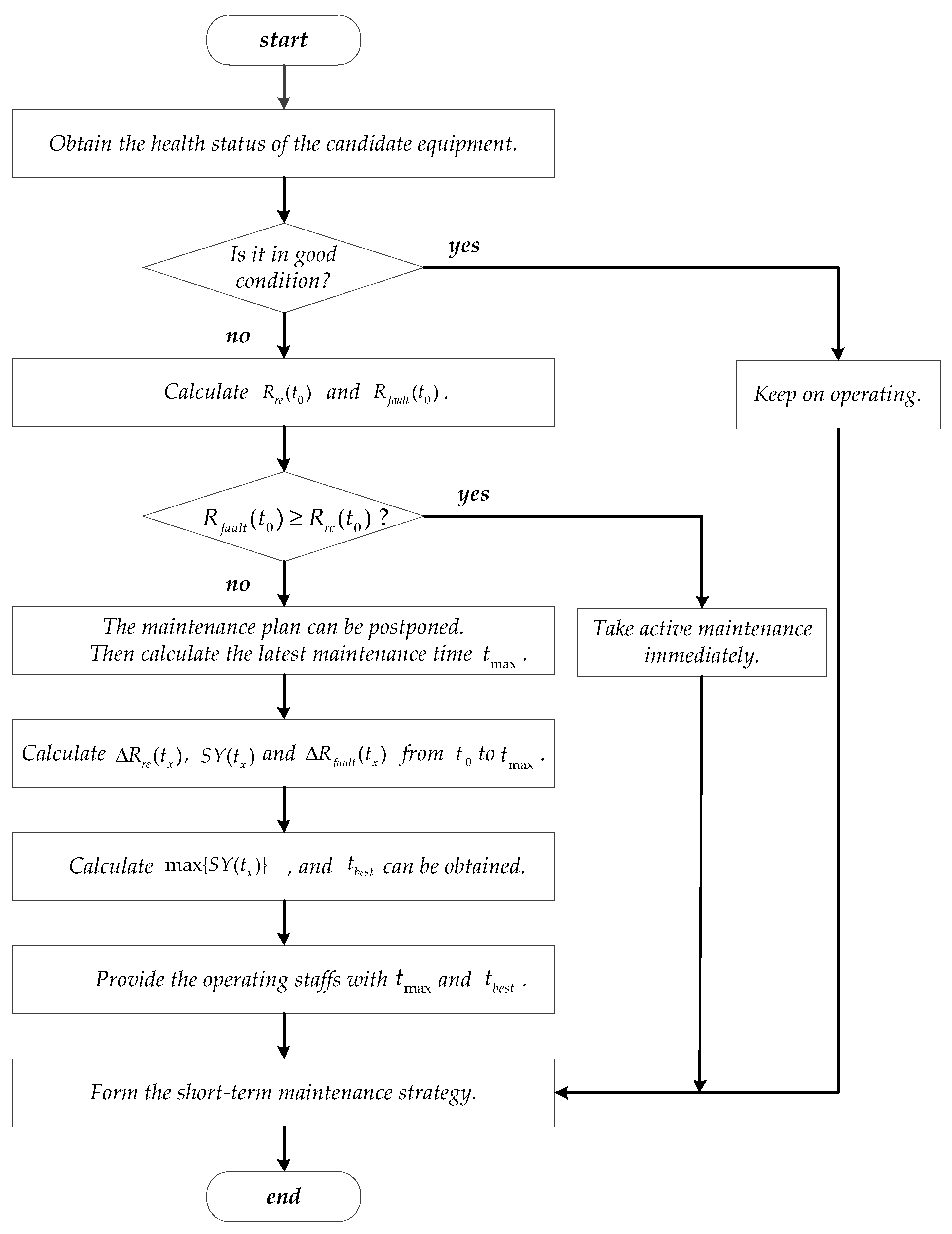
Figure 3.
The structure diagram of IEEE 24-bus system.

Figure 4.
Simulation results of bus 17 at 24:00 (a) Load forecasting results of bus 17; (b) Load shedding results of bus 17.
Figure 4.
Simulation results of bus 17 at 24:00 (a) Load forecasting results of bus 17; (b) Load shedding results of bus 17.

Figure 5.
Curves of operation risk costs and active maintenance costs.
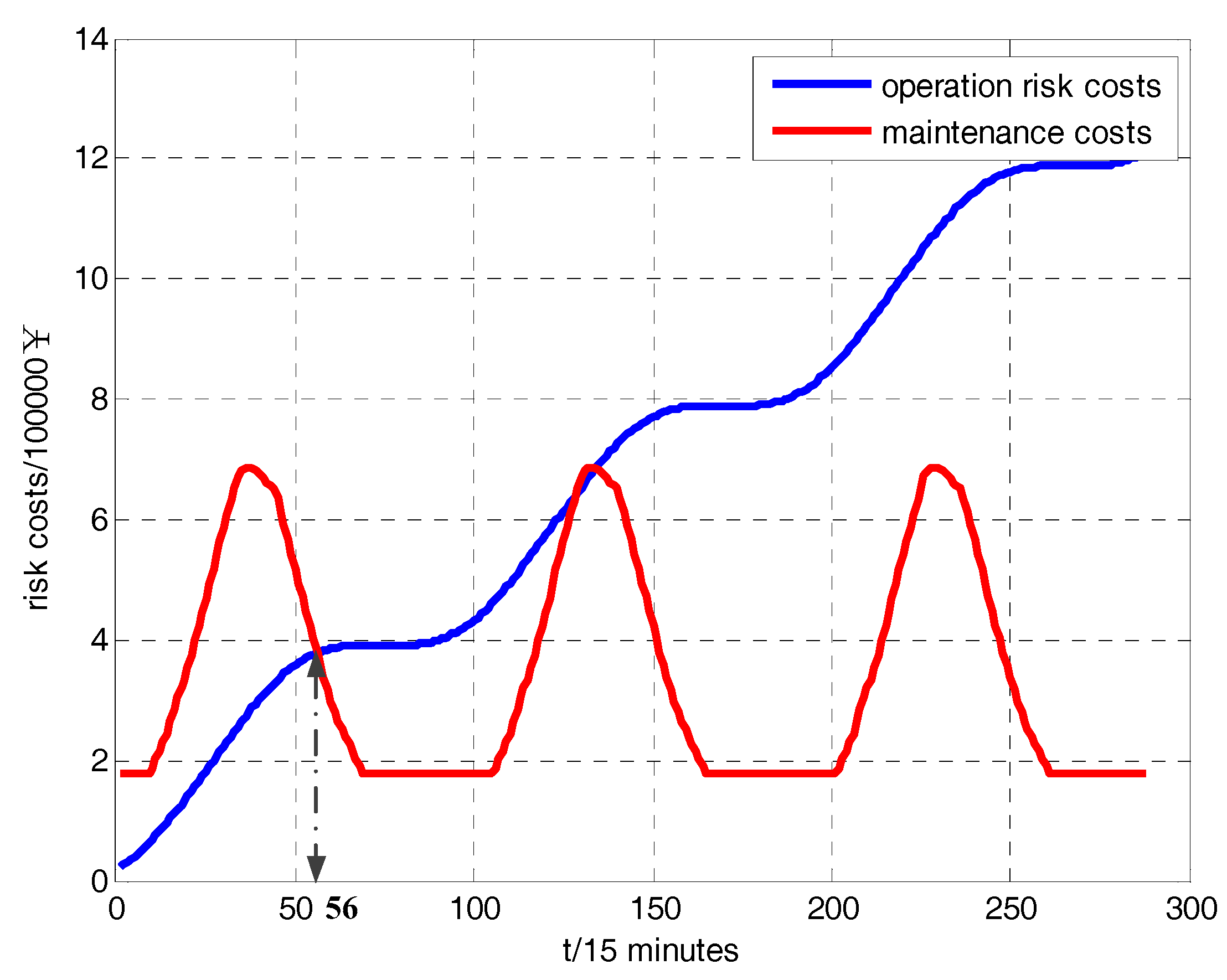
Figure 6.
Diagram of the relative earnings of the next 14 h.
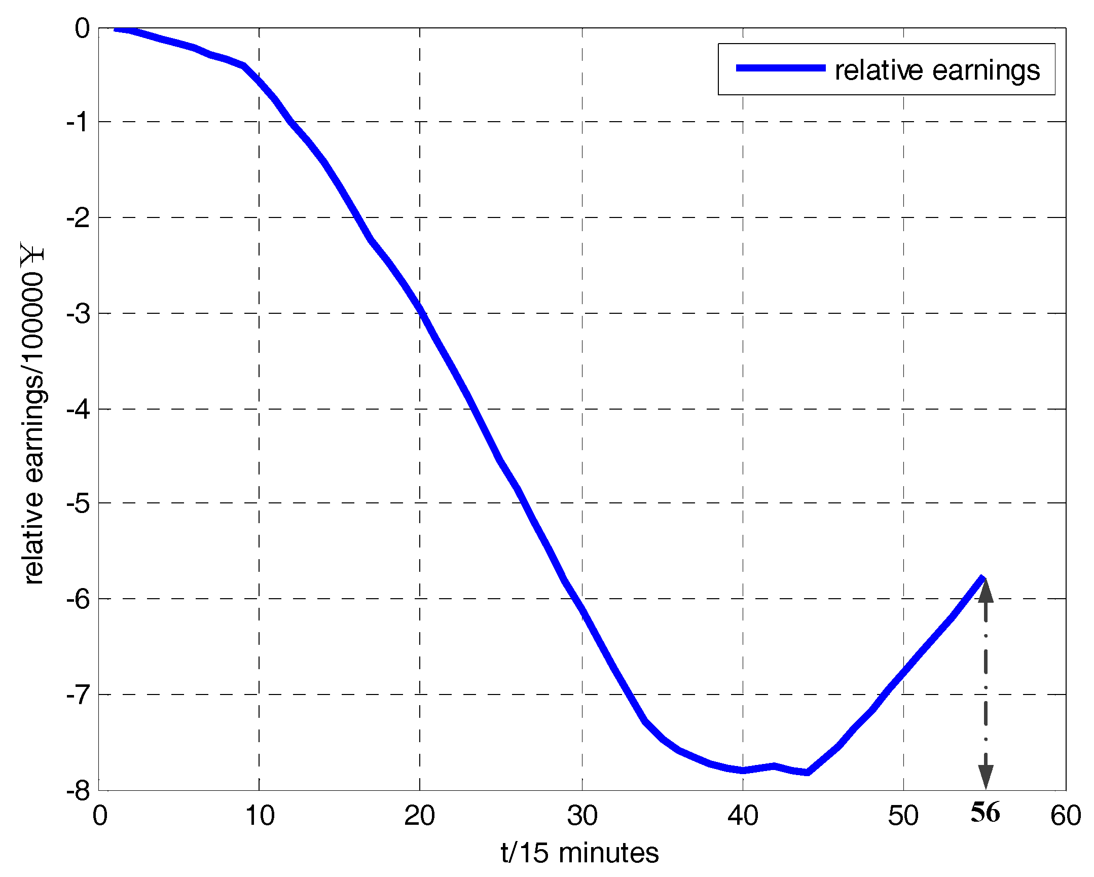
Figure 7.
Simulation results of bus 17 at 19:00 (a) Load forecasting results of bus 17; (b) Load shedding results of bus 17.
Figure 7.
Simulation results of bus 17 at 19:00 (a) Load forecasting results of bus 17; (b) Load shedding results of bus 17.
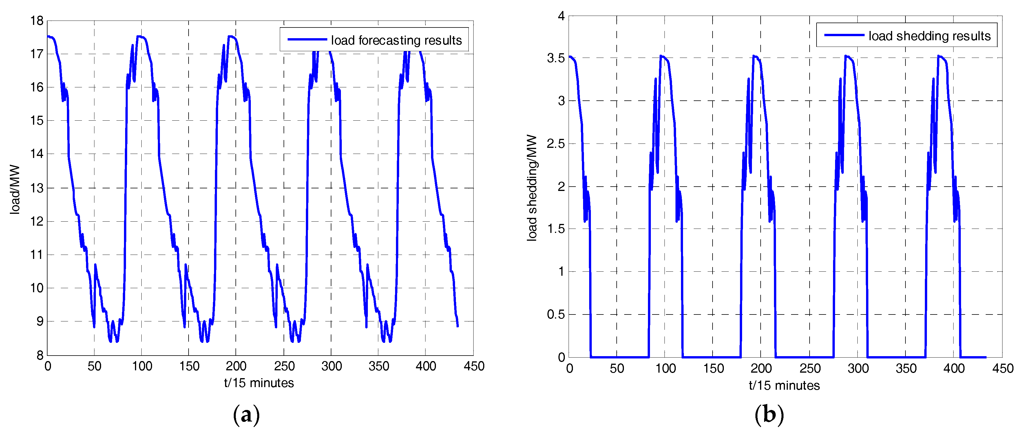
Figure 8.
Curves of operation risk costs and maintenance costs.

Figure 9.
Diagram of the relative earnings of the next 9 h.

Table 1.
The electric power price data.
| Items | Electric Power Price/(¥/kWh) | ||
|---|---|---|---|
| Peak Period: 17:00–22:00 | Flat Period: 9:00–17:00 | Valley Period: 23:00–7:00 | |
| pbuy | 0.3 | 0.3 | 0.3 |
| psell−1 | 1.67 | 1.3 | 1.1 |
| psell−2 | 1.43 | 1.21 | 0.99 |
| psell−3 | 1.13 | 0.91 | 0.62 |
| ppenalty−1 | 5.01 | 3.9 | 3.3 |
| ppenalty−2 | 4.29 | 3.63 | 2.97 |
| ppenalty−3 | 3.39 | 2.73 | 1.86 |
© 2017 by the authors. Licensee MDPI, Basel, Switzerland. This article is an open access article distributed under the terms and conditions of the Creative Commons Attribution (CC BY) license (http://creativecommons.org/licenses/by/4.0/).
Share and Cite
MDPI and ACS Style
Yang, H.; Zhang, Z.; Yin, X.; Han, J.; Wang, Y.; Chen, G. A Novel Short-Term Maintenance Strategy for Power Transmission and Transformation Equipment Based on Risk-Cost-Analysis. Energies 2017, 10, 1865. https://doi.org/10.3390/en10111865
AMA Style
Yang H, Zhang Z, Yin X, Han J, Wang Y, Chen G. A Novel Short-Term Maintenance Strategy for Power Transmission and Transformation Equipment Based on Risk-Cost-Analysis. Energies. 2017; 10(11):1865. https://doi.org/10.3390/en10111865
Chicago/Turabian StyleYang, Hang, Zhe Zhang, Xianggen Yin, Jiexiang Han, Yong Wang, and Guoyan Chen. 2017. "A Novel Short-Term Maintenance Strategy for Power Transmission and Transformation Equipment Based on Risk-Cost-Analysis" Energies 10, no. 11: 1865. https://doi.org/10.3390/en10111865
Note that from the first issue of 2016, this journal uses article numbers instead of page numbers. See further details here.