An Integrated Modeling Approach for Forecasting Long-Term Energy Demand in Pakistan

Abstract

Energy planning and policy development require an in-depth assessment of energy resources and long-term demand forecast estimates. Pakistan, unfortunately, lacks reliable data on its energy resources as well do not have dependable long-term energy demand forecasts. As a result, the policy makers could not come up with an effective energy policy in the history of the country. Energy demand forecast has attained greatest ever attention in the perspective of growing population and diminishing fossil fuel resources. In this study, Pakistan’s energy demand forecast for electricity, natural gas, oil, coal and LPG across all the sectors of the economy have been undertaken. Three different energy demand forecasting methodologies, i.e., Autoregressive Integrated Moving Average (ARIMA), Holt-Winter and Long-range Energy Alternate Planning (LEAP) model were used. The demand forecast estimates of each of these methods were compared using annual energy demand data. The results of this study suggest that ARIMA is more appropriate for energy demand forecasting for Pakistan compared to Holt-Winter model and LEAP model. It is estimated that industrial sector’s demand shall be highest in the year 2035 followed by transport and domestic sectors. The results further suggest that energy fuel mix will change considerably, such that oil will be the most highly consumed energy form (38.16%) followed by natural gas (36.57%), electricity (16.22%), coal (7.52%) and LPG (1.52%) in 2035. In view of higher demand forecast of fossil fuels consumption, this study recommends that government should take the initiative for harnessing renewable energy resources for meeting future energy demand to not only avert huge import bill but also achieving energy security and sustainability in the long run.

1. Introduction

Developing countries around the globe are striving to ensure supplies of economical, sustainable and if possible cleaner form of energy for meeting their energy demand. As such, medium to long term energy demand forecasts are inevitable to catch up economic growth and social development based on realistic estimates [1]. It is extremely important for energy planning and management (energy production and distribution) that these forecasts should be based on precise forecasting models [2,3]. Developing energy demand forecasting model, which is anticipated to provide a reliable forecast, is challenging as it depends on various data inputs pertaining population, economy and technologies [4]. From a methodological perspective, a variety of co-integration techniques, neural and abductive network techniques, multivariate modeling and univariate time series analysis such as the autoregressive moving average (ARMA) modeling is extensively employed in the literature for energy demand forecast. A list for various energy demand forecasting studies with scope, forecasting methodologies used and time horizon in various countries is shown in

Table 1. Literature reporting energy demand forecasting.

Reference	Scope	Country/Location	Forecasting Method	Forecasting Horizon
[2]	Electricity	Lebanon	ARIMA	monthly
[6]	Primary energy demand	Turkey	ARIMA	2005–2020
[7]	Electricity	Turkey	ARIMA	2005–2014
[8]	Natural gas	Turkey	ARIMA	2008–2030
[9]	energy consumption	Turkey	ANN and regression analyses	2008–2014
[10]	Natural gas	Turkey	ARIMA, ANN moreover, neuro fuzzy system	weekly
[4]	Energy consumption	China	grey forecasting model and genetic programming	1990–2007
[11]	CO2 emissions, energy consumption and economic growth	Brazil	Grey prediction model	2008–2013.
[12]	Energy demand	Taiwan	SARIMA model	2010–2020
[13]	Electricity price and demand	Finland	ARIMA and neural networks	day-ahead
[14]	Energy demand	USA	ANN, regression analysis Models and ARIMA	2014–2019
[15]	Oil, gas and total energy consumption	China	Group method of data handling (GMDH) and GMDH based auto-regressive (GAR) model.	2014–2020
[16]	Demand Forecast of Natural Gas	Sakarya, Turkey	time series decomposition, Holt-Winters, exponential smoothing and ARIMA	Year Ahead
[17]	Energy demand	Nigeria	ARIMA and ETS model	2012–2030
[18]	Energy consumption in road transportation	China	ETS & ARIMA models and multiple regression models	2012–2020
[19]	Electricity	Pakistan	Holt-Winter and ARIMA	2012–2020
[20]	Energy consumption	China	Comparison of ARIMA model and GM(1,1) model	2014–2020
[21]	Energy demand	10 Asean countries	Log-linear and quadratic models	1991–1995
[22]	Energy demand and supply	Taiwan	LEAP	2008–2030
[23]	Electricity Demand	South Australia	semi-para-metric additive models	2009–2019

. Most of these forecasting model take into account variables such as Gross Domestic Product (GDP), income, degree-days, population and energy price to estimate energy demand [2,5].

In this study, three different energy demand forecasting methods, i.e., Autoregressive Integrated Moving Average (ARIMA), Holt-Winter and Long-range Energy Alternate Planning (LEAP) model have been used to project energy demand up to 2035. The demand forecast estimates of each of these methods were compared using annual energy demand data as tons of oil equivalents (TOE). ARIMA model was first described by Box and Jenkins [24] for forecasting univariate time series data. On the other hand, LEAP is a software-based energy modeling tool which is used explicitly for energy planning and policy analysis having excellent simulation capabilities.

Energy demand forecasting is extremely important for Pakistan to undertake effective energy planning and policy development for the nation which essentially requires reliable and sustainable energy supplies for progress in all the sectors of the economy [25,26,27]. In this context, this research is an attempt to fulfil the persisting gap relating to reliable energy demand forecasting in the country. This study is first of its kind work which energy demand forecasting for all major fuels and for all of the sectors of the economy for a period of 21 years (2015–2035). In the subsequent parts of this paper an overview of energy system in Pakistan is provided in Section 2 including historical energy demand and supply in Pakistan, the power and energy demand forecasting efforts made in Pakistan, Economic growth and energy consumption in Pakistan, description of methodological and theoretical framework in the Section 3, results and discussion in Section 4 and Section 5 provides conclusion with s policy recommendation.

2. Overview of the Energy System in Pakistan

2.1. Historical Energy Demand and Supply

Pakistan is located in South Asia and bordered by Afghanistan, Iran, India and China with a total area of 803,940 km² of which 97% is land area while rest is covered by water [28]. For the past couple of decades, the energy crisis is hindering economic growth in the country. Amongst all energy resources, electricity have had received greater attention owing to fast growth in its demand [29]. The government is under considerable pressure to overcome energy crisis thereby investing in the sector and maintaining the economic growth at the same time [30]. It was until the 1980’s when Pakistan was able to meet its energy demand indigenously sufficiently. Although, in 1990’s new discoveries of oil and gas were made, however, later they even become insufficient to fulfil the growing energy demand of the nation. As a result in the year 2000, Pakistan started importing a significant amount of energy resources with crude oil leading imported fuel [31]. As of today, the critical state of Pakistan’s energy sector is a primary constraint on the country’s economic development. Despite sufficiently important contribution found in the literature to address issues in the energy sector and various options suggested therein for overcoming energy crisis, the energy sector of Pakistan has not recovered as yet with evident supply and demand gap and various other challenges encountered [32].

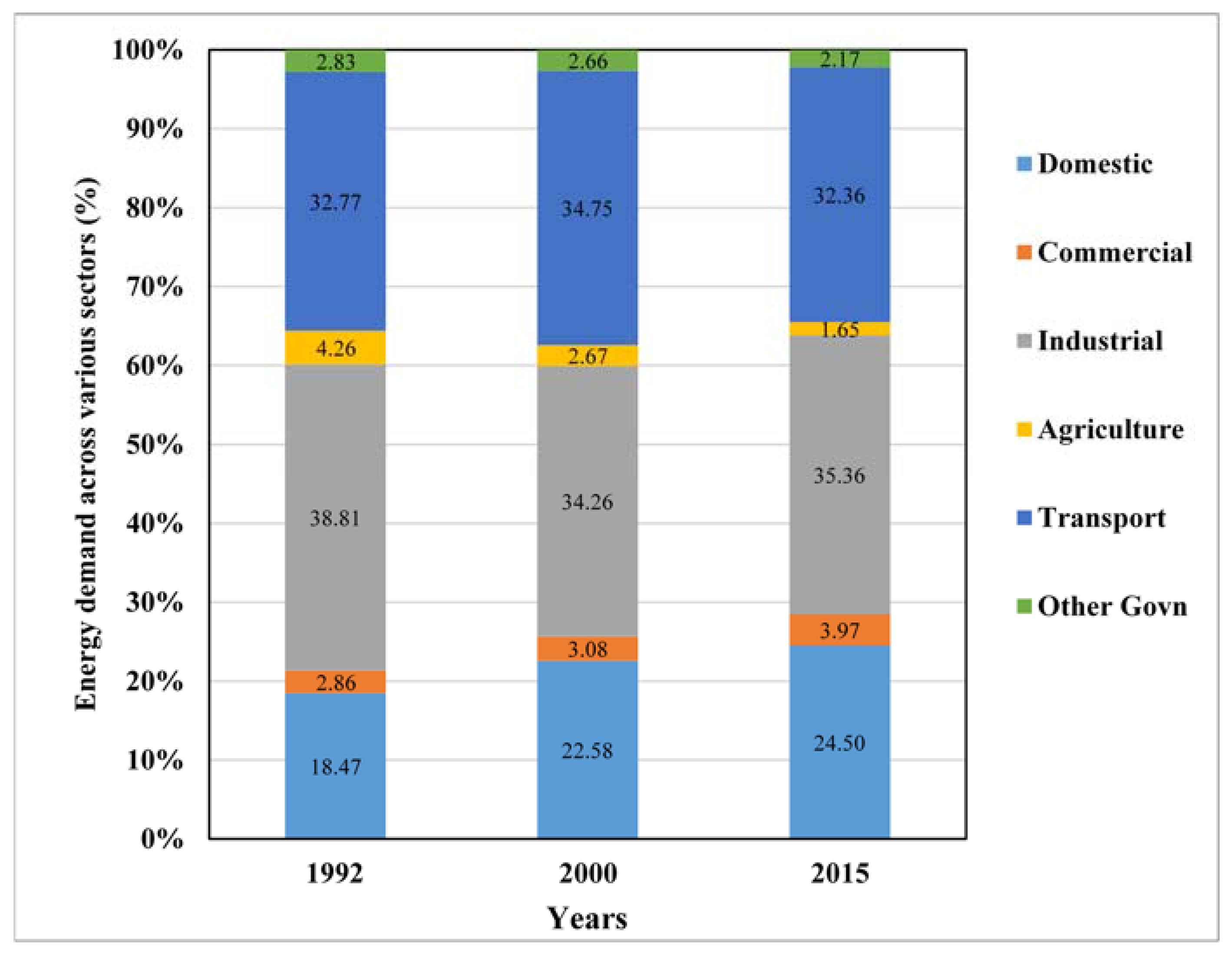
According to the energy statistics published by HDIP, the primary commercial energy supplies of the Pakistan was 70 million TOE in 2015. The share of each source in primary energy supplies for 2014–2015 was oil: 35.5%, gas: 42.7%, LPG: 0.7%, LNG imported: 0.7%, coal: 7.0% and imported electricity: 0.2%. On the other hand, the highest share in total energy demand is coming from industrial sector (35.36%), followed by transport sector (32.36%), domestic sector (24.50%) and commercial sector (3.97%) as shown in (Figure 1). The indigenous oil produced in 2015 was at the rate of 94,493 barrels per day while natural gas statistic remained 4016 MMCFD in 2014. A total of 47 exploratory and 35 development/appraisal wells were drilled. On the other hand, the oil import bill for the year 2014–2015 was US$12 billion. New hydel power plants of 438 MW capacity was also installed during this period. The total electricity generation for the same period was 106,966 GWh, which was comprised of 63.5% from the thermal power plant, 30.4% from hydel plants, 5.4% from the nuclear power plant and only 0.7% from renewable sources [33]. The historical consumption of different fuels across different sectors of the economy shows that oil and gas have been the most dominant fuels since 1992. The transport sector has been the main consumer of oil while natural gas consumption has raised over the past few years owing to enhanced supplies to the power sector and demand from domestic sector.

The main causes of current energy crisis are mainly attributed to decades old poor policy inconsistent fuel mix for the various sector of the economy as evident from data in

Table 2. Energy fuel mix across various sectors from 1992 to 2015.

Fuel Type		Domestic	Commercial	Industrial *	Agriculture	Transport	Other Govt.
Oil	1992	8.56%	0.42%	15.48%	3.39%	68.25%	3.90%
	2000	4.12%	0.00%	17.35%	2.55%	72.97%	3.01%
	2015	0.66%	0.00%	9.45%	0.28%	86.84%	2.77%
Natural gas	1992	31.48%	5.81%	62.70%	0.00%	0.01%	0.00%
	2000	40.47%	6.28%	52.55%	0.00%	0.70%	0.00%
	2015	41.30%	5.23%	43.60%	0.00%	9.88%	0.00%
Coal	1992	0.22%	0.00%	99.78%	0.00%	0.00%	0.00%
	2000	0.04%	0.00%	99.96%	0.00%	0.00%	0.00%
	2015	0.00%	0.00%	100.00%	0.00%	0.00%	0.00%
Electricity	1992	33.82%	6.33%	36.27%	17.26%	0.09%	6.23%
	2000	47.06%	5.58%	28.96%	9.96%	0.03%	8.40%
	2015	48.30%	7.59%	29.11%	9.36%	0.00%	5.64%
LPG	1992	0.00%	0.00%	0.00%	0.00%	0.00%	0.00%
	2000	75.00%	25.00%	0.00%	0.00%	0.00%	0.00%
	2015	41.33%	41.16%	0.00%	0.00%	0.00%	17.51%

* Power generation has been included in industrial sector.

. As a result of these poor policies [34]; mostly thermal power plants in the private sector were commissioned from the period 1994–2000 with no major hydropower project undertaken during this period. The electricity produced from these thermal power units is very costly and the government had to offer subsidies which further deteriorated the economic conditions of the country [35]. As a result of these policies, Pakistan’s present electricity generation is mainly from oil and gas with a very limited contribution from coal-fired plants. In order to avoid the power generation sector being vulnerable to the global energy market, it is inevitable to transform country’s generation mix [36,37]. The amount of energy import forecasted for Pakistan by various researchers shows that the country will face serious challenges with regards to energy supply and price shocks in future. This implies that some serious efforts are required to transform energy sector by diversifying local production, improving energy efficiency and follow conservation practices to avoid unbearable oil and gas import bills [38]. More recently as well as historical energy consumption pattern suggests that energy growth rate shall persist at an annual growth rate of 8.8% which would require 361 million tons of oil equivalent (MTOE) of energy by 2030. In other words, Pakistan has to enhance energy production by almost six times to that of the supply level of 2010-2011 (64 MTOE) [39].

There have been some efforts from the Government of Pakistan (GOP) to promote the adoption of renewable energy technologies (RETs). In this context, first, ever renewable energy policy of the country was announced in 2006. However, implementation of this policy faced various challenges thus had achieved only limited success [40]. In recent times, Ministry of Water and Power developed a balanced power policy in 2013 that aimed at dealing energy crisis with balanced fuel mix and energy conservation also could not deliver to the expectation of the various sectors of the economy [41]. As a result, despite of these efforts, in 2013 and 2014 worst sort of energy and power crises were coped with 16 to 18-hour of electricity supply interruptions [42].

The energy supply targets can be generally achieved if demand is projected appropriately thus enabling the government to develop long-term integrated energy plans including the future arrangements for energy supplies. Unfortunately, Pakistan so far have had been unable to devise integrated energy plan taking into consideration any of fairly estimated demand forecast. Most of the demand forecast studies at government level are generally exaggerated, such as such as Government of Pakistan [43] study which estimated energy demand projection for future. This study had estimated energy demand forecast for Pakistan as of 120.18 million TOE in 2015 which actually came out to be 70 million TOE. Importantly no parallel matching efforts are visible to devise and implement integrated energy plan for the country based on the demand forecast studies.

2.2. Power and Energy Demand Forecasting Efforts

Integrated energy modeling, as the process of energy planning and policy development has had rarely been undertaken in Pakistan. Although, there are some studies conducted in this context both by government and academia. At the government level, studies such as Government of Pakistan [43], Petroleum Institute of Pakistan [44], National Transmission and Dispatch Comparny Limited [45] are more prominent and academia contribution include Hussain, Rahman and Memon [19], Perwez, et al. [46], Perwez and Sohail [47], International Resources Group [48], Hussain, et al. [49], Anwar [50], Anwar [51]. Most of the studies have generally forecasted electricity demand for various sectors of the economy over different time horizons. There are other studies by Anwar [51], Government of Pakistan [43], Petroleum Institute of Pakistan [44], Anwar [50] and International Resources Group [48] which mostly discusses different aspects of energy systems in general. Nevertheless, in this section of the paper, some of important studies wherein power and energy demand forecast have been undertaken are discussed in further detail.

Water and Power Development Authority (WAPDA), a fully government controlled department announced the first comprehensive Power Plan for the country in 1994. The plan comprises of load forecast, generation planning and transmission expansion planning for the period from 1992 to 2018. This plan was subsequently further updated in 1995, 1996, 1998, 2003, 2008, 2011, 2012 and in 2014. The latest regression based load forecast report was prepared by National Transmission and Dispatch Comparny Limited [45] in 2014 and is based on the historical data which encompasses electricity consumption, electricity tariff, GDP and population. The electricity demand forecast in latest study extends up to the year 2037 and includes three demand scenarios which are low growth scenario (3.56% GDP growth), normal growth scenario (5% GDP growth) and high growth scenario (6.5% GDP growth). The data used for Regression Analysis entailed GDP by major sectors (agriculture, manufacturing, trade, services, etc.), category wise electricity consumption, tariff wise price of electricity, category wise consumers and load shedding data of PEPCO and K-Electric, Consumer Price Index (CPI) and population. In the process of regression analysis, the elasticity coefficients are calculated at first and followed by application Ordinary Least Squares (OLS) method of estimation for regression analysis. Electricity consumption (GWh) for various consumer categories including domestic, commercial, industrial and agricultural were selected as dependent variables. Some 51 different regression models were developed and tested with a different combination of response variables.

Perwez and Sohail [47] developed three long-term energy pathways to meet the forecasted electricity demand. The three scenarios of this study are Business As Usual (BAU), New Coal (NC) and Green Futures (GF). Long-Range Energy Alternative Planning (LEAP) software was used to forecast electricity demand and develop supply side scenario for the period 2011–2030. Since, the data required for the final energy intensity was not available for Pakistan, as such, this study used total annual consumption and number of electric consumer in each sector to obtain the final energy intensity. In another study by Petroleum Institute of Pakistan [44] aimed at presenting Pakistan energy outlook used single and multiple independent variables and undertook regression analysis to predict energy demand for residential, industrial, commercial, agriculture and transport sectors up to 2025. The independent variable selection in this study was based on trial and error process so that best fit variables were determined. Further, the residuals of the last observation (the difference between actual and predicted numbers) were added in some cases for smoothing the previous years’ effect. The regression equations used to obtain the results are given as under:

(a)

Primary energy/capita = 0.024 + 2.831 Real GDP/Capita + Residual,

(b)

Residential Electricity demand/connection = 673 + 0.012 Real GDP/Capita + Residual,

(c)

Residential sector Natural gas demand: From 2014, onwards the demand for natural gas/customer is being considered at 2014 level with an increase in gas connections by 5% each year,

(d)

Residential sector LPG: LPG spend = 0.286 × Natural gas spend,

(e)

Residential sector oil: Oil spend = 26,306 − 0.433 × LPG spend,

(f)

Industrial fuel demand: Industrial fuel demand = 1.373 + 0.0001 Real GDP Manufacturing,

(g)

Transport Sector Fuel: Road Transport Demand = −6.550 + 0.276 Real GDP + 0.093 Population − 0.045 Fuel Prices,

(h)

Commercial Electricity Spend = 10,287 + 9.007 Real GDP Services + Residual; Commercial Natural Gas = −7532 + 2.572 Real GDP Services,

(i)

Commercial sector LPG + Gas spend = −24,917 + 5.886 Real GDP Services + Residual,

(j)

Agriculture and Government Electricity spend = 7.651 Real GDP + Residual and

(k)

Agriculture and Government fuel spend = 2.118 Real GDP + Residual.

Similarly, Anwar [50,51] projected the service energy demand through three different techniques: (i) econometric models (ii) relating energy service demand in particular sector to GDP and (iii) relating energy service demand to value added of the particular sector. Service energy demand in transport and the residential sector was determined through econometric approach using dependent variables such as a number of energy devices, passenger kms, ton km and others to be dependent on independent variables such as Gross Domestic Product (GDP) and population. On the other hand, service energy demand in industrial, commercial and agriculture sector was projected through economic value added and GDP approach. In this case, the service demand of particular sector in particular year is considered equal to service demand of that sector in the base year multiplied by the ratio of the current year GDP and base year GDP. The Service demand projection for agriculture, commercial and industrial sector was based on the service demand of sector in the base year multiplied by the ratio of the current year value added and base year value added.

2.3. Economic Growth and Energy Consumption

Renewable and non-renewable energy consumption is an important determinant of economic growth like other factors of production such as labor and capital. The literature on energy and growth nexus is generally divided in four competing hypotheses which are: growth hypothesis, conservation hypothesis, feedback hypothesis and neutrality hypothesis [52]. The energy demand is a function of various factors such as real income, relative prices and structure of the economy, the available technology and lifestyle [53]. Economic growth is closely related to growth in energy consumption because more energy used result the higher the economic growth [54]. Like other developing countries, Pakistan is also growing energy intensive economy, as such, the per capita energy consumption is increasing with time as shown in

Table 3. Historical energy use profile of Pakistan [56].

Years	Population (Million)	Total Primary Energy (MMTOE)	Power Gen. Installed Capacity (MW)	Natural Gas Consumption (MMcfd)	Energy Consumption per Capita (MMBtu)
1950	35	1.4	115	0	1.7
1960	45	3.0	425	60	2.9
1970	60	6.4	1700	300	4.5
1980	81	12.5	3500	711	6.5
1990	108	28.0	9000	1364	10.9
2000	140	42.0	17,000	1950	12.5
2001	143	44.5	17,000	2104	13.0
2002	146	45.2	17,758	2259	13.0
2003	149	47.1	17,793	2390	13.2
2004	153	50.8	19,252	2881	13.9

. Further, like most of the other non-oil producing countries, energy needs of Pakistan are met by large quantities of imports. Thus, to meet its growing energy demand, Pakistan faces both energy constraints from the supply side as well as dare demand management at the same time [55].

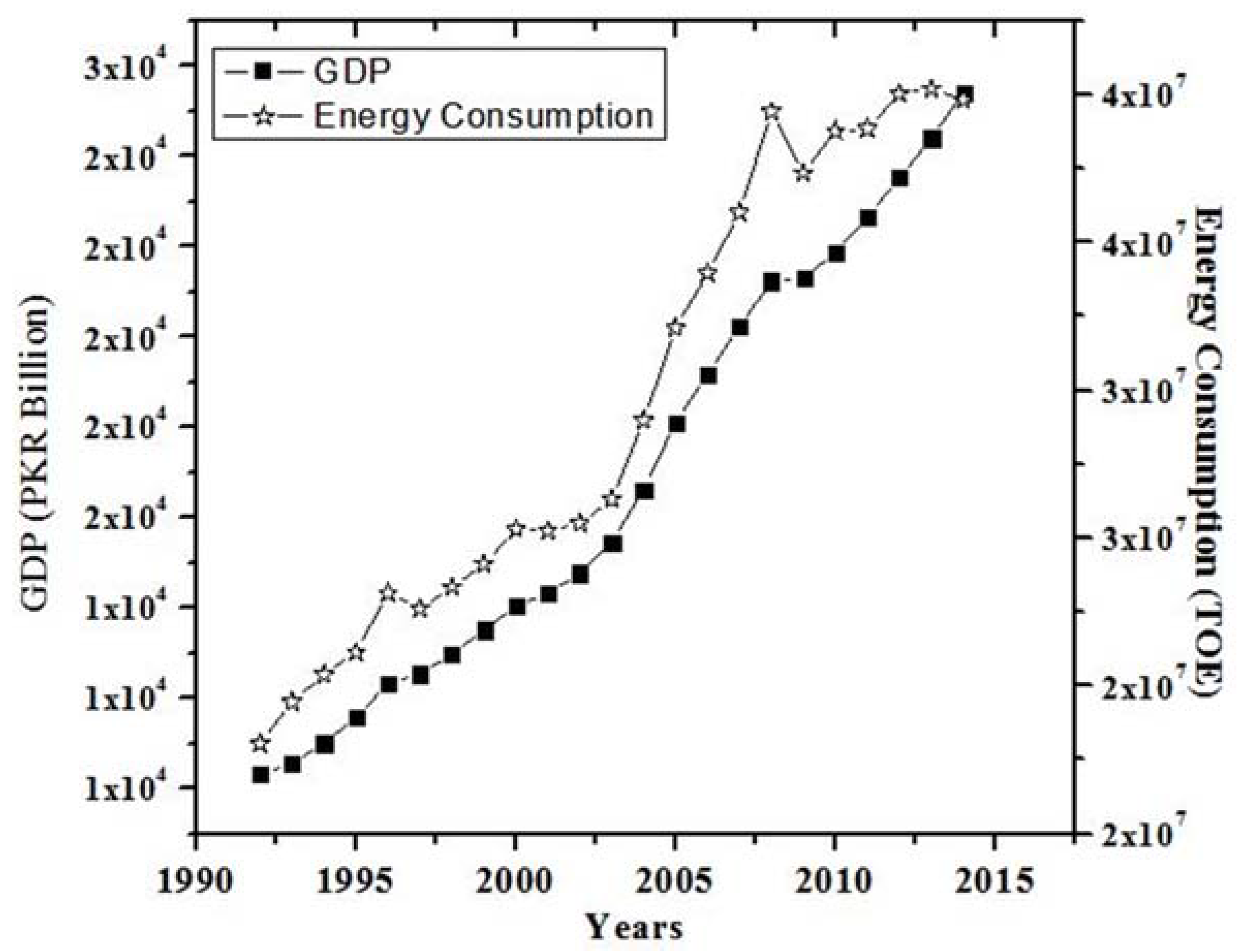
Pakistan’s economy generally remained stable during the period 2001–2007 with fairly strong GDP growth of 5.4%. A remarkable GDP growth of 8.9% was recorded for the year 2005. However, the rate of GDP growth fell drastically by 0.36% in 2009 which resulted in low energy consumption, i.e., 37.3 MTOE which was 39.4 MTOE in 2008. The slowdown in economic activity caused energy consumption to decline [57] and vice versa as shown in Figure 2. According to Alahdad [32], by assuming an annual economic growth rate of 6.5%, an energy supply of 198 million TOE shall be required in order to meet the demand in 2025.

A large number of studies have been undertaken to test the relationship of demand (consumption) of different energy commodities i.e., electricity, oil, natural gas, coal with various economic indicators. These studies for Pakistan, have also tested the classical theories and hypothesis of energy economics. In this context, numerous important studies that reflect the relationship between energy consumption and energy-economic nexus for Pakistan have been carried out (Aqeel and Butt [55]; Siddiqui [58]; Nasir and Ur Rehman [59]; Khan and Ahmad [53]; Shahbaz and Lean [60]; Hye and Riaz [61]; Shahbaz, Zeshan and Afza [52]; Zaman, et al. [62]; Raza, et al. [63]; Ahmed, et al. [64]; Komal and Abbas [65]; Shahbaz, et al. [66]; Shahbaz, et al. [67] and Arshad, Zakaria and Junyang [31]).

Some authors have also reported the GHG emissions as a function of energy consumption and economic growth in Pakistan. Alam, Fatima and Butt [54] indicated that a 1% increase in economic growth, in the long run, will increase CO₂ emissions by up to 0.84%. Ali and Abbas [68] have estimated CO₂ emission from energy consumption as direct and indirect emissions. Nasir and Ur Rehman [59] found that 1% increase in per capita real GDP will increase per capita emissions by 7.20% in the long-run. Similarly, 1% increase in per capita energy consumption may lead to 1.65% increase in per capita carbon emissions. This brings forth the important finding that besides the contribution of energy with stimulation of economic activities, energy consumption also contributes to emissions through some non-economic activities of, for example, domestic and transport sectors. Importantly, together these two sectors consume almost 50% of total energy in Pakistan. As such, energy policy makers in should not only focus on forecasting the future demand for energy with different growth scenarios but also on focusing the least cost energy options.

3. Methodological and Theoretical Framework

The historical energy demand (consumption) data of six sectors (domestic, industrial, commercial, transportation, agriculture and other government sectors) and five fuels (electricity, oil and petroleum, natural gas, coal and LPG) have been retrieved from Pakistan’s energy yearbooks published annually by Hydrocarbon Development Institute of Pakistan (HDIP). The data mentioned above from energy yearbooks was converted into time series data starting from 1992 till 2014. Subsequently, the energy demand forecast of all these sectors of the economy for each fuel using each ARIMA, Holt-Winter and LEAP methodology was undertaken.

3.1. Autoregressive Integrated Moving Average (ARIMA) and Holt-Winter Approach

The abbreviation ARIMA has been derived from the two models involved in the methodology, i.e., Autoregressive model (AR) and the Moving Average model (MA) [12,69]. ARMA methodology has been used in this study to model the stationary time series with an appropriate number of $p$ and $q$ lags [2,11]. ARMA focuses on the stochastic, or probabilistic properties of economic time series on their own instead of constructing single or simultaneous equation models. The model considers the stochastic error terms and is based on the own past or lagged values. The ARMA ($p, q$) model when written as ARIMA ($p, d, q$) will mean that the series has been made stationary by differencing it “d” times. This is important because either ARIMA model is applied in a series which is stationary or by applying a certain order of difference so that it becomes stationary for forecasting [7,11]. The Holt-Winter approach analysis the trend and seasonal variation in the time series data along with exponentially smoothed component. The optimal utilization of this methodology is to estimate the Root Mean Square Error (RMSE) and Mean Absolute Percent Error (MAPE), which is one of the most widely used approaches to test and validate the model outcomes.

The historical publication of Box and Jenkins [24] and the later sequels of the same publication provides the stepwise procedure for the ARMA analysis [8,69]. The step followed in this are same as of followed in various studies. These are:

(1) Time series data is differentiated in order to make it stationary first which is achieved by making both variances and mean constant [10];

(2) Determining p and q orders by studying the autocorrelation and partial autocorrelation coefficients [13,14];

(3) Validating the selected models by applying diagnostic tests that provide information about the residuals being white noise [2,8]. Detail of each of these steps is given under:

If the means, variances and covariances of the series are independent of time, rather than the entire distribution, then the time series data is said to be stationary [70,71]. On the other hand, the non-stationarity in a series might originate due to various reasons. Amongst which the most important one is the occurrence of “unit roots”. For instance, as shown below, the autoregressive model of order 1 with lag 1 [19,20]:

$$Y_t=\theta Y_{t-1}+{\varepsilon }_t$$

(1)

where Y_t is any time series, θ is the coefficient, ε_t stands for an error term serially uncorrelated white noise having a zero Mean and a fixed variance. The Equation (1) will become a random walk without a drift in the model if θ = 1. Therefore, the problem of “unit root” arises when θ = 1 in real series which in fact mean that the series is non-stationary. On the other hand, if |θ| ≤ 1, then the series Y_t is considered stationary. The stationarity series is checked at first stage because correlation might exist in non-stationary time series and even in very large sample which results into the spurious (or nonsense) regression [7,72]. From Equation (1) it is inferred that wherever the issue of unit root arises in the time series, the differencing is done and is therefore indicated as the order of integration for each series. The objective at the back of co-integration is that if a linear combination of nonstationary variables is stationary then the variables are said to be co-integrated. Thus, the linear combination cancels out the stochastic trends in two series and, as a result, the regression would be meaningful; i.e., not spurious [7].

The next step is to determine suitable p and q orders for autoregressive (AR) and moving average (MA) segments of the ARIMA [7,10,11]. This is done by analyzing auto-correlation function (ACF) and partial auto-correlation function (PACF) [16,73]. It is achieved by using statistical software EVIEWS (version 7). The ACF and PACF also provided a statistical summary at a particular lag. Maximum count of lags was determined by dividing the number of observations by 4, as each of our series had less than 240 observations according to Box and Jenkins method. Since the number of observations in this study is 23 and the lag number is calculated as 6. One of the most important tools is the visualization of time series graphs and then observing the correlogram specifically. This correlogram of auto-correlation and partial auto-correlation provided information about the appropriate orders of MA and AR respectively drawn on the basis of lags involved [6,8]. The resulting correlograms are simply the plots of ACF and PACF against the lag length. The ACF at lag k, denoted by ${\rho }_k$, is defined as [7,8]:

$${\rho }_k=\frac{{\gamma }_k}{{\gamma }_0}$$

(2)

where γ_k is the covariance at lag k, γ₀ is the variance. Since both covariance and variance are measured in the same units, ${\rho }_k$ is a unitless—or pure—number and lies between −1 and +1. In time series data, the main reason of correlation between Y_t and Y_t−k originates from the correlations they have with intervening lags, i.e., Y_t−1, Y_t−2, …., Y_t−k+1. The partial correlation measures the correlation between observations that are k time periods apart after controlling for correlations at intermediate lags, i.e., it removes the influence of these intervening variables. In other words, partial auto-correlation is the correlation between Y_t and Y_t−k after removing the effect of intermediate Y’s [19].

Further, before finally selecting a forecasting model, the residuals from the estimation is observed in the previous step and checked whether any of the auto-correlations and partial correlations of the residuals are individually and statistically significant or not. They are being statistically significant, meaning that the residuals were purely random and there was no need to look for another ARIMA model. In the final step, forecasting was carried out based on the developed and checked ARIMA model [7]. The Minitab tool (version 14) was used in this study, without seasonal variation, to forecast the time series [69] for the next 21 observations, i.e., up to 2035.

The forecasting outcomes of the ARIMA and Holt-Winter models have been validated by the so-called “within sample forecasting capability” using two different tests: Root Mean Square Error (RMSE) and Mean Absolute Percentage Error (MAPE). The mathematical relationship of both RMSE and MAPE is given below [12,15,19,74]:

$$\mathrm{RMSE}=\sqrt{\frac{{\sum }_{i=1}^n\left|{\left(F_i-A_i\right)}^2\right|}{n}}$$

(3)

$$\mathrm{MAPE}=\left(\frac{{\sum }_{i=1}^n\left|(F_i-A_i/A_i\right|}{n}\right)\times 100\%$$

(4)

where A_i is the actual value and F_i is the forecasted value. The forecasting results of ARIMA and Holt-Winter models are matching which are discussed in detail in Section 4 of this paper. It may be noted that estimated RMSE and MAPE for every time series have been used in this study. Out of the total 28 time-series analyzed, 11 series have both RMSE and MAPE higher in ARIMA compared to Holt-Winter, while 9 series have RMSE and MAPE smaller in ARIMA. However, the decision that which model is a most appropriate model is taken on the basis of RMSE only which is smaller in 15 series forecasted through ARIMA as compared to Holt-Winter approach as shown in

Table 4. Error measures of ARIMA and Holt-Winter Forecasting Models.

Holt-Winter Model			ARIMA Model
Oil
Sectors	RMSE	MAPE		RMSE	MAPE
Domestic	40,360.85	347,009.36	Domestic	40,896.30	374,545.26
Industrial	254,528.21	17,204,692.08	Industrial	193,848.31	19,926,731.58
Agriculture	9775.32	599,696.77	Agriculture	22,980.84	41,108.95
Transport	268,490.99	203,712,749.62	Transport	259,924.42	218,744,031.58
Other Govt.	17,779.68	7,833,528.41	Other Govt.	14,824.40	7,334,826.32
Thermal power	799,149.33	202,166,666.67	Thermal power	873,683.20	204,652,515.79
Total	619,458.79	226,401,119.29	Total	281,050.96	242,497,542.11
Natural Gas
Sectors	RMSE	MAPE		RMSE	MAPE
Domestic	315,295.30	117,830,812.05	Domestic	393,505.23	114,615,089.47
Commercial	32,735.15	20,261,815.06	Commercial	18,380.76	19,377,231.58
Industrial	828,429.06	194,360,295.26	Industrial	973,411.45	200,360,263.16
Transport	337,027.50	62,030,631.58	Transport	298,615.33	60,139,600.00
Thermal power	1,740,446.33	62,030,631.58	Thermal power	1,430,927.80	203,392,026.32
Fertilizer	398,245.11	98,858,980.12	Fertilizer	361,241.98	97,500,131.58
Cement	4496.79	303,019.88	Cement	73,340.75	3,186,778.95
Total	779,996.9699	388,296,359.8	Total	1,318,376.63	409,063,684.2
Coal
Sectors	RMSE	MAPE		RMSE	MAPE
Industrial	438,146.90	98,032,343.63	Industrial	312,017.10	91,851,315.79
Thermal power	15,141.33	1,630,728.77	Thermal power	10,236.35	1,355,226.84
Total	434,584.06	97,932,298.32	Total	327,510.99	91,443,421.05
Electricity
Sectors	RMSE	MAPE		RMSE	MAPE
Domestic	43,111.70	64,145,330.99	Domestic	74,797.57	66,065,505.26
Commercial	4276.77	10,279,323.34	Commercial	5206.46	10,389,873.68
Industrial	106,535.38	33,991,791.15	Industrial	98,136.80	34,248,889.47
Agriculture	65,271.88	16,938,946.78	Agriculture	46,860.02	16,212,347.37
Other Govt.	23,407.44	9,303,922.66	Other Govt.	24,986.82	9,348,942.11
Total	71,061.12	135,683,521.63	Total	157,556.11	140,742,305.26
LPG
Sectors	RMSE	MAPE		RMSE	MAPE
Domestic	203,069.01	14,637,104.24	Domestic	199,105.33	14,344,631.58
Commercial	11,302.71	4,804,046.78	Commercial	20,044.11	5,273,536.84
Other Govt.	18,101.41	537,305.26	Other Govt.	16,751.25	606,368.42
Total	42,618.53	12,917,467.84	Total	67,738.42	14,105,568.42

Other govt.: Other government sectors.

.

In addition, for ARIMA model, experiments on 24 different time series was carried out one by one. As such, following analysis of the auto-correlogram and partial auto-correlogram, the best parameter settings for each energy consumption of the time series used are determined as given in

Table 5. Description of ARIMA parameters applied in each forecasted time series.

Sectors	Fuel Type	Parameters ARIMA (p,d,q)	Sectors	Fuel Type	Parameters ARIMA (p,d,q)
Domestic	Electricity	ARIMA (1,1,4)	Domestic	Natural Gas	ARIMA (1,1,4)
Industrial	Electricity	ARIMA (1,2,4)	Industrial	Natural Gas	ARIMA (1,2,5)
Commercial	Electricity	ARIMA (1,1,5)	Commercial	Natural Gas	ARIMA (1,1,5)
Agriculture	Electricity	ARIMA (2,1,3)	Transportation	Natural Gas	ARIMA (2,1,5)
Transportation	Electricity	ARIMA (1,1,3)	Thermal Power	Natural Gas	ARIMA (2,1,4)
Other Govt.	Electricity	ARIMA (1,1,3)	Domestic	Coal	ARIMA (1,1,2)
Domestic	Oil	ARIMA (2,1,5)	Industrial	Coal	ARIMA (2,1,5)
Industrial	Oil	ARIMA (1,1,2)	Thermal Power	Coal	ARIMA (2,1,3)
Commercial	Oil	ARIMA (2,1,3)	Domestic	LPG	ARIMA (2,1,3)
Agriculture	Oil	ARIMA (1,1,4)	Commercial	LPG	ARIMA (1,1,4)
Transportation	Oil	ARIMA (4,1,3)	Other Govt.	LPG	ARIMA (1,1,2)
Other Govt.	Oil	ARIMA (2,1,2)
Thermal Power	Oil	ARIMA (2,1,2)

[15]. The consumption/demand of certain fuels some sectors of the economy are being recorded zero, as such, there is no ARIMA model in such case. Similarly, the power generation sector consumes a significant amount of oil and natural gas, therefore, has been considered as a separate sector of the economy.

Generally, ARIMA modeling technique only requires data for the modelled variable, thus saving the user from the trouble of determining influential variables [2]. It is known that if θ = 1, i.e., in the case of unit root, Equation (1) becomes a random walk model without drift which is known as non-stationary process. The basic idea behind the unit root test of stationary is to simply regress Y_t on its (one-period) lagged value Y_t−1 and find out if the estimated θ is statically equal to 1 or not [17]. Ducky Fuller test (DF) is applied to check whether the data is stationary or non-stationary. By stationarity, it is meant that the series with constant mean and constant variance. In this study, the Augmented Ducky Fuller Test (ADF) has been used for checking unit root problem.

$$\begin{array}{l}\mathsf{\Delta }{Y}_t={\alpha }_t+{\beta }_t+\rho Y_{t-1}+{\epsilon }_t\\ H_0:\rho =0\\ H_1:\rho \le 0\end{array}$$

(5)

where H₀: series is non-stationary; H₁: Series is stationary; A Series is said to be stationary if it satisfying following properties; (a) the process has fixed mean i.e., $E(y_t)=\mu$ and (b) the process is homoscedastic or constant variance i.e., $Var(y_t)={\sigma }^2$. The covariance between two observations of series depends on the lag between the two observations but not on the time index t. i.e., $covar(y_t, y_{t-j})={\sigma }_j$.

In ADF test, the lags of the first difference are included in the regression in order to make the error term ε_t white noise and, therefore, the regression is presented in the following form:

$$\mathsf{\Delta }{Y}_t=\delta Y_{t-1}+{\alpha }_i{\displaystyle \sum }_{i=1}^m\mathsf{\Delta }{Y}_{t-1}+{\varepsilon }_t$$

(6)

To be more specific, we may also include an intercept and a time trend t, after which model becomes:

$$\mathsf{\Delta }{Y}_t={\beta }_1+{\beta }_{2}t+\delta Y_{t-1}+{\alpha }_i{\displaystyle \sum }_{i=1}^m\mathsf{\Delta }{Y}_{t-1}+{\varepsilon }_t$$

(7)

The DF and ADF tests are similar since they have the same asymptotic distribution. In literature, there are various unit root tests. However, the most notable and commonly used one is ADF test and, therefore, it has been used in this study [7].

3.2. The Long-Range Energy Alternatives Planning (LEAP) Tool

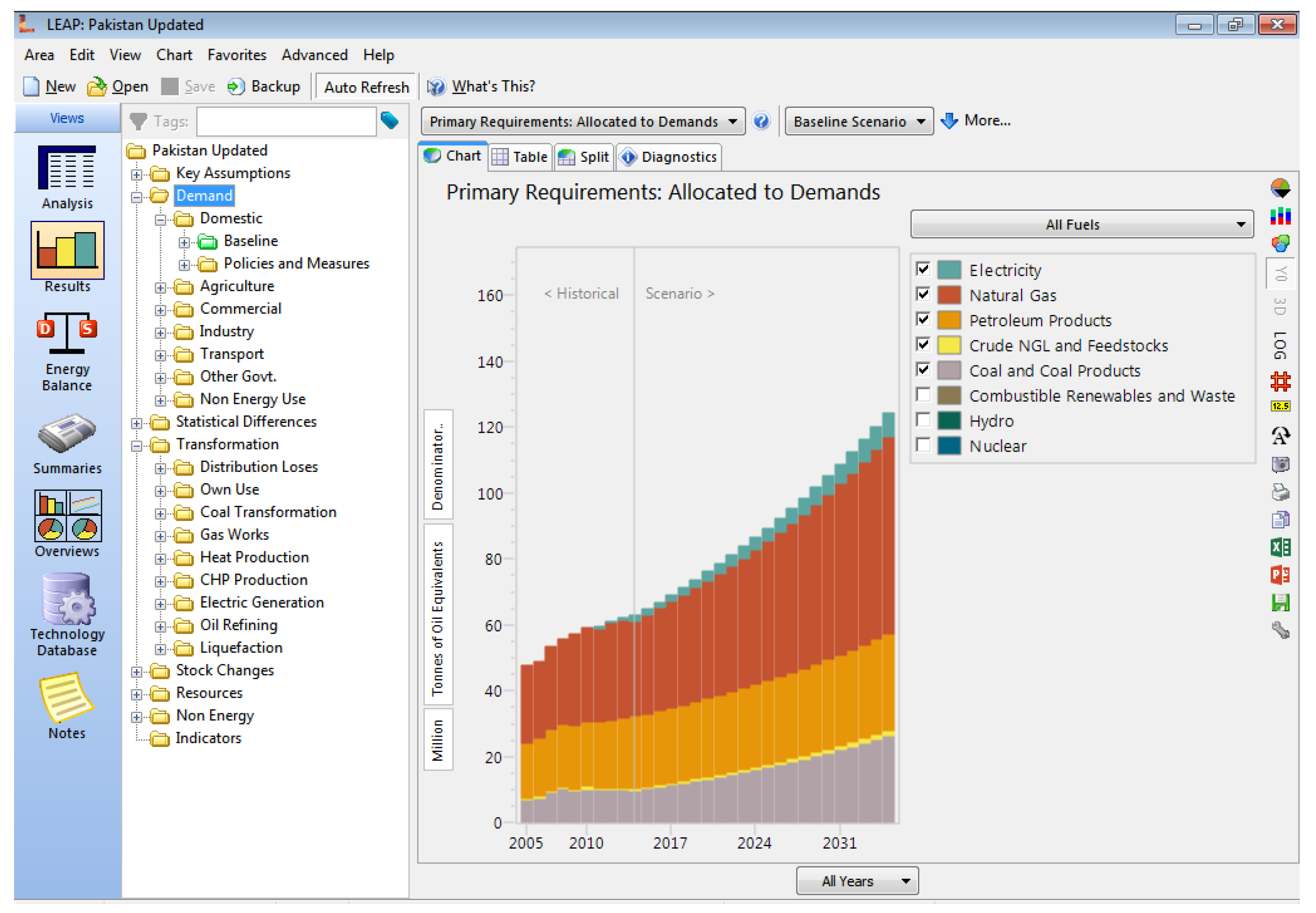
The Long-range Energy Alternatives Planning (LEAP) is a software-based modeling tool that allows simulation of energy systems for specific applications suited to particular problems at various spatial levels (cities, state, country, region or global). LEAP incorporates both demand and supply side features of the system being an integrated energy planning model (Figure 3). In this study, we have used the demand forecasting features of the LEAP model. The model contains various mathematical and statistical functions that follows the accounting framework to forecast energy demand based on the time series data provided to the software. The demand analysis, following the end-use approach, is carried out as follows [75]:

• The analysis is carried out sector by sector having the time series energy demand data of each fuel called demand devices that is defined by the user. Thus, a “hierarchical tree,” is generated; where the higher branches of the tree sums up the energy demand of all lower branches. This hierarchy might consist of: sectors, sub-sectors, end-uses and fuels/devices.
• In most of the cases, the product of activity and the energy intensity (i.e., demand per unit of the activity) is used to obtain the demand at the disaggregated levels. However, the model allows alternative options and in our case, we used the linear forecasting function to obtain results that were based on the time series historical data used in this study.

The LEAP modeling interface is highly flexible and can perform analysis at any spatial or temporal scale [5]. In the current study, we neither used the economic parameters to forecast energy demand nor energy intensity—instead, we used the time series linear forecasting capability of the model so that we could compare the results with the other two models, which are also based on time series secondary data.

One of the main advantages of LEAP is that, it can be used with minimal data for demand forecasting using the in-built modeling tools in the software. However, the modeler can perform complex analysis by constructing sophisticated relationships between exogenous variables and energy systems variables. Such analysis requires more data that are added to the system in the form of key assumptions for which the user set equations in order to obtain useful results.

4. Results and Discussions

In this study, three different energy demand forecasting methodologies namely ARIMA, Holt-Winter and Long-range Energy Alternate Planning (LEAP) model were used to forecast energy demand for the period 2015–2035. In the first instance, the results obtained from the ARIMA model—which provided the most appropriate results for the energy demand—are analyzed. The ARIMA forecasting model produced results in three different patterns which are upper limits, lower limits and forecasted values. Upper and lower limits provide a confidence interval of 95%, in other words, any realization within the confidence limits will be acceptable. Therefore, we have provided the forecasted values only in the form of data tables (below the figures) and as such in the tabular format alone. This is in order to bring simplicity in the presentation i.e., we have omitted the upper and lower limits. Similarly, the values mentioned in the respective tables and figures lies within the 95% confidence interval limits [6]. The results show that industrial sector will have the highest energy demand in 2035, i.e., 40.84 million TOE as shown in

Table 6. Total forecasted energy consumption by Sector (TOE) from 2015 to 2035.

Year	Domestic	Commercial	Industrial	Agriculture	Transport	Other Govt.	Total
2015	9,939,306	1,791,296	33,642,419	764,450	12,692,419	811,936	59,641,826
2020	11,566,993	2,062,227	32,987,225	806,300	14,100,015	889,659	62,412,419
2025	13,126,796	2,356,714	33,960,092	864,430	15,738,020	948,017	66,994,069
2030	14,736,824	2,651,746	37,312,592	932,979	17,319,592	1,004,315	73,958,048
2035	16,329,066	2,946,828	40,843,417	993,811	18,943,822	1,061,002	81,117,946

Other govt.: Other government sectors.

followed by transport sector (18.94 million TOE) and domestic sector (16.32 million TOE). However, a major portion of the industrial sector energy demand will be from thermal power plants which is estimated as 21.01 million TOE.

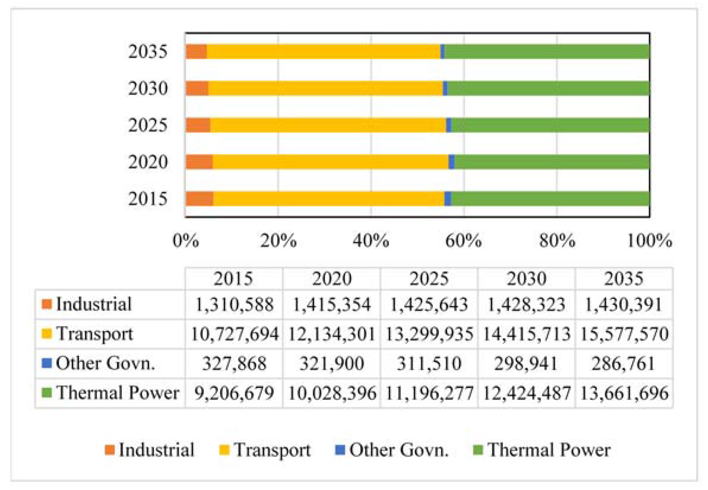
The results further suggest that energy fuel mix will be dominated by the oil (38.16%) in 2035 with a total demand of 30.9 million TOE as shown in Figure 4. The highest demand for oil will be from transport sector which is estimated to be 15.5 million TOE followed by thermal power plants 13.6 million TOE. The oil demand in domestic and agriculture sectors have been omitted from Figure 4 because ARIMA has forecasted negative oil demand in these sectors due to historically declining trend.

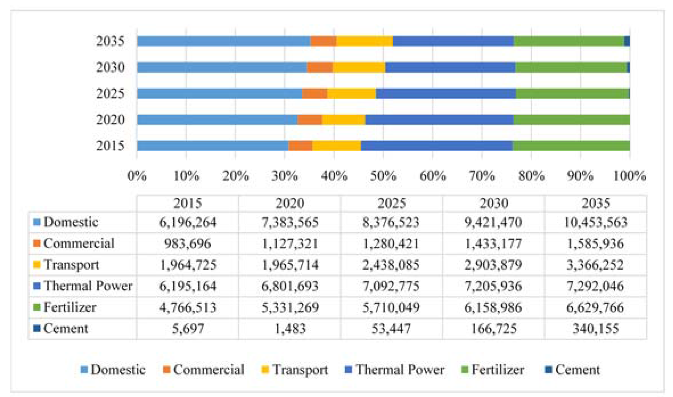
Amongst other fuels, natural gas is forecasted to be second most demanding fuel. Natural gas demand in the country is forecasted to rise continuously and is estimated to reach 29.66 million TOE in 2035 as shown in Figure 5. The main consumer of natural gas will be domestic sector (10.4 million TOE) followed by thermal power plants (7.2 million TOE). Natural gas consumption in industrial subsectors—except for the fertilizer, cement and power production sectors—shall be declining. It is important to mention that most of the natural gas consumed in the industrial sector is forecasted to produce electricity for the industry’s own use called captive power.

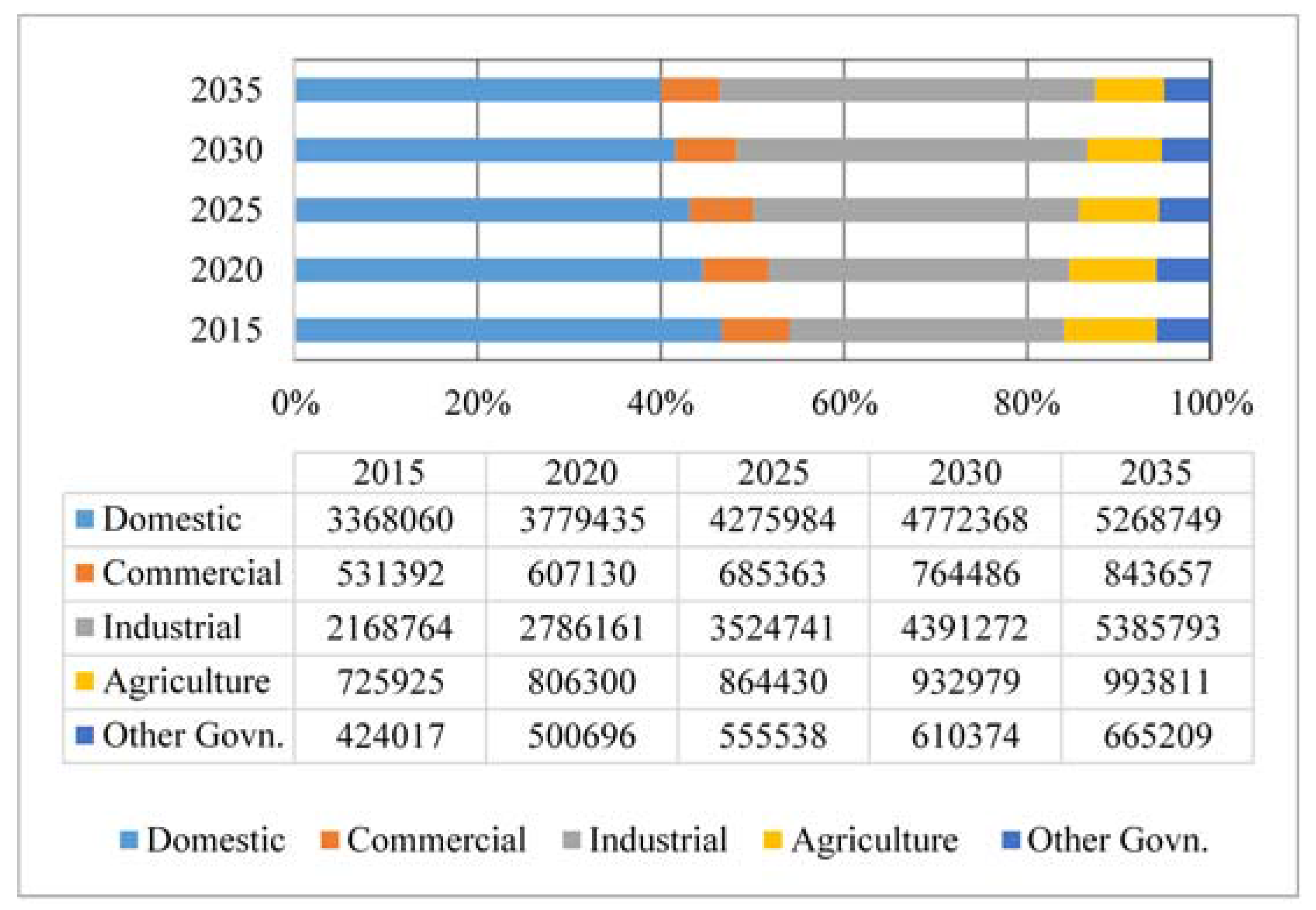
From the results of ARIMA model of this study, it is estimated that by the end of forecasting period, i.e., 2035, electricity share in total fuel mix shall be 17.74% which corresponds to 13.1 million TOE and most of the electricity is projected to be consumed in industrial sector (5.3 million TOE), followed by domestic (5.2 million TOE), agriculture (0.9 million TOE) and commercial (0.8 million TOE) sectors as shown in Figure 6.

The electricity demand forecasted by Hussain, Rahman and Memon [19] for Pakistan using ARIMA model from 2015 to 2020 closely match with the results of this study as shown in

Table 7. Comparison of Electricity forecasted by Hussain, Rahman and Memon [19] and this study (GWh).

	Years	Domestic	Commercial	Industrial	Agriculture	Other Govt.
This study	2015	39,171	6180	25,223	8443	4931
[19]	2015	40,820	6647	26,088	10,020	5210
This study	2020	43,955	7061	32,403	9377	5823
[19]	2020	47,046	7724	32,377	11,209	5843

Other govt.: Other government sectors.

. The National It is worth mentioning here that Energy Security Plan (NESP) developed by the government of Pakistan for period 2005–2030 had also envisaged the increased demand for fossil fuels for meeting the future energy needs. With some of LPG import projects, it was forecasted that the overall energy import share of the country would increase from the existing 31 to 45% by 2030. Accordingly, in terms of power requirements, it was forecasted that the electricity demand would reach 163 GW, of which 44.6 GW would be shared by alternative energy resources, including hydro, nuclear and renewable by 2030 [76].

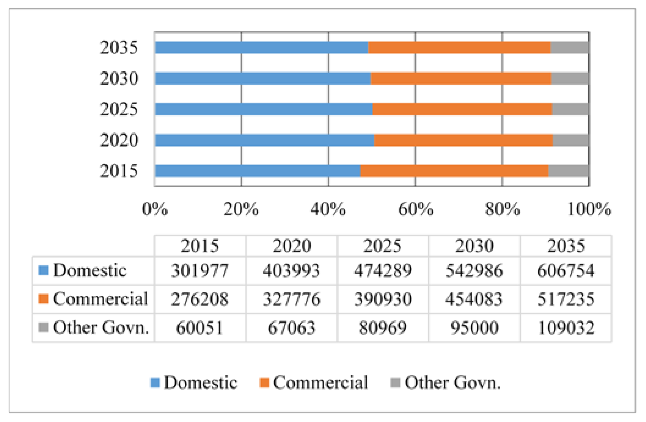
The share of coal and LPG in both current and future energy mix is low, i.e., this study results revealed that coal and LPG would share 8.23% and 1.66% of the fuel mix in 2035 respectively. This implies that the demand for coal and LPG in 2032 will be 6.1 and 1.23 million TOE respectively as shown in Figure 7 and Figure 8. The main consumption of coal is forecasted for the industrial sector while LPG demand shall be high in the domestic sector.

The share of each source in primary energy supplies for 2014–2015 remained as oil: 35.5%, natural gas: 42.7%, LPG: 0.7%, LNG imported: 0.7%, coal: 7.0% and imported electricity: 0.2% [33]. These shares of each fuel for different sectors in total energy consumption varies considerably from base year (2014) till the end of forecasting period (2035) as of alone oil from 35 to 50% in industrial, 32 to 23% in transport sector, 25 to 20% in domestic sector, 2 to 1% in agriculture sector and 2% to 1% in other government sectors. This variance in fuel consumption during the base year (2015) and the end year of forecasting (2035) is owing to the fact that, contrary to the conventional position of a single fuel for one sector, a variety of fuels shall be in demand from different sectors. For instance, domestic sectors wherein generally electricity and natural gas is in demand shall also be consuming LPG during the forecast period as shown in

Table 8. Energy demand forecast across domestic sector depicting various fuels (million TOE).

Year	Oil *			Natural Gas *			Fuel Wood	LPG †			Electricity *
	ARIMA ‡	LEAP	Holt-Winter	ARIMA ‡	LEAP	Holt-Winter	LEAP	ARIMA ‡	LEAP	Holt-Winter	ARIMA ‡	LEAP	Holt-Winter
2010	0.093	0.091	0.093	5.134	5.028	5.134	25.499	0.942	0.923	0.942	2.791	2.734	2.791
2015	0.073	0.105	0.068	6.196	6.366	6.599	28.642	0.302	0.262	0.572	3.368	3.256	3.311
2020	−0.16	0.117	−0.11	7.384	7.089	7.479	31.890	0.404	0.292	0.685	3.779	3.625	3.761
2025	−0.39	0.129	−0.29	8.377	7.808	8.359	35.127	0.474	0.322	0.797	4.276	3.993	4.212
2030	−0.51	0.141	−0.47	9.421	8.521	9.240	38.334	0.543	0.351	0.910	4.772	4.358	4.662
2035	−0.67	0.152	−0.66	10.454	9.232	10.120	41.533	0.607	0.380	1.022	5.269	4.721	5.112

*: Holt-Winter results are more appropriate; ^†: ARIMA results are more appropriate; ^‡: (within 95% CI limits).

.

It is evident from

Table 9. Energy demand forecast across Industrial sector depicting various fuels (million TOE).

Year	Oil †			Natural Gas *			Coal †				Electricity †
	ARIMA ‡	LEAP	Holt-Winter	ARIMA ‡	LEAP	Holt-Winter	ARIMA ‡	LEAP	Holt-Winter	ARIMA ‡		LEAP	Holt-Winter
2010	0.998	0.983	0.998	8.710	8.574	8.710	4.282	4.215	4.282	1.614		1.589	1.614
2015	1.311	1.614	1.328	6.225	8.700	6.701	3.696	4.261	3.251	2.169		2.452	2.089
2020	1.415	2.079	1.439	2.341	11.206	4.981	4.211	5.488	2.178	2.786		3.159	2.617
2025	1.426	2.652	1.550	−3.68	14.291	3.262	4.892	6.999	1.105	3.525		4.028	3.144
2030	1.428	3.354	1.661	−11.81	18.074	1.542	5.471	8.851	0.032	4.391		5.095	3.672
2035	1.430	4.212	1.772	−22.01	22.699	−0.18	6.041	11.116	−1.04	5.386		6.399	4.199

*: The Holt-Winter results are more appropriate; ^†: ARIMA results are more appropriate; ^‡: (within 95% CI limits).

that there is a minor difference in the forecasting results of ARIMA and Holt-Winter models, yet the most appropriate model selection is only considered subject to model validation exercise. However, in case of more conservative approach, the negative forecasted values can be neglected by considering LEAP estimates for planning purposes.

The forecasting results of this study suggest that industrial sector shall be a major consumer of different energy commodities with a demand of 40.84 million TOE in 2035 as shown in Table 9 and

Table 10. Energy demand forecasts * for Industrial and sub-industrial sector (million TOE) ^‡.

	Industry				Thermal Power			Cement	Fertilizer	Total
	Oil	Electricity	Coal	Natural Gas	Oil	Natural Gas	Coal	Natural Gas	Natural Gas
1992	1.34	1.00	1.37	3.30	2.72	4.19	0.018	0.275	1.96	16.2
2000	2.07	1.08	1.26	4.25	6.07	4.80	0.156	0.200	3.48	23.4
2010	9.98	1.61	4.28	8.71	8.60	7.11	0.0561	0.045	4.28	35.7
2015	1.31	2.17	3.70	6.23	9.21	6.20	0.0674	0.006	4.77	33.6
2020	1.42	2.79	4.21	2.34	10.0	6.80	0.0704	0.001	5.33	33.0
2025	1.43	3.52	4.89	-	11.20	7.09	0.0656	0.053	5.71	34.0
2030	1.43	4.39	5.47	-	12.40	7.21	0.0660	0.167	6.16	37.3
2035	1.43	5.39	6.04	-	13.7	7.29	0.0625	0.340	6.63	40.8

^‡: The results are ARIMA based only; *: (within 95% CI limits).

. However, the rising energy demand for all fuels and all sub-sectors within the industrial sector cannot be taken for granted. It is pertinent to mention that as per results of this study suggest that Pakistan is not only currently importing oil in huge quantities but the similar trend may continue onwards as huge quantities of oil are used for electricity generation which contributes to overall fuel consumption of the industrial sector. The natural gas, which has been so far indigenously produced with diminishing tended and may exhaust until further reserves are not discovered. Therefore, natural gas supply to industrial activities other than power production has been minimized with continuous decline.

The transport sector, throughout the forecasting period, is mainly oil dependent with 15.57 million TOE demand in the year 2035 following by natural gas demand of 3.36 million TOE as shown in

Table 11. Energy demand forecast across transport sector (million TOE).

Year	Oil †			Natural Gas †
	ARIMA ‡	LEAP	Holt-Winter	ARIMA ‡	LEAP	Holt-Winter
2010	9.338	9.077	9.338	2.317	2.252	2.317
2015	10.728	10.933	10.865	1.965	2.060	1.756
2020	12.134	11.787	13.124	1.966	2.221	0.283
2025	13.300	12.547	15.382	2.438	2.364	−1.19
2030	14.416	13.356	17.641	2.904	2.517	−2.66
2035	15.578	14.218	19.899	3.366	2.679	−4.14

^†: ARIMA results are more appropriate; ^‡: (within 95% CI limits).

. It is noted that over past decade, a large number of the vehicle have switched their fuel from oil to natural gas which has caused an imbalance of supply of this commodity in great demand in the industrial and domestic sector. As a result, during the winter when natural gas demand in the domestic sector rises, the load shedding of natural gas is observed in the transport sector thus oil is indispensable fuel for the transport sector.

In the commercial sector, the demand for natural gas, electricity and LPG shall be increasing with each commodity demand estimated 1.58, 0.78 and 0.42 million TOE respectively in 2035 and the demand for oil is projected to be decreasing as shown in

Table 12. Energy demand forecasts in commercial sector depicting (various fuels million TOE).

Year	Natural Gas †			LPG *			Electricity *
	ARIMA ‡	LEAP	Holt-Winter	ARIMA ‡	LEAP	Holt-Winter	ARIMA ‡	LEAP	Holt-Winter
2010	0.865	0.804	0.865	0.209	0.194	0.209	0.457	0.425	0.457
2015	0.984	0.965	0.913	0.276	0.264	0.253	0.531	0.562	0.531
2020	1.127	1.367	1.016	0.328	0.375	0.294	0.607	0.796	0.592
2025	1.280	1.912	1.119	0.391	0.524	0.336	0.685	1.113	0.653
2030	1.433	2.675	1.223	0.454	0.733	0.377	0.764	1.557	0.714
2035	1.586	3.743	1.326	0.517	1.026	0.419	0.844	2.179	0.774

*: Holt-Winter results are more appropriate; ^†: ARIMA results are more appropriate; ^‡: (within 95% CI limits).

.

Electricity is the key energy commodity in demand in the agriculture sector mainly for irrigation tube wells and forecasted to be 0.99 TOE in 2035. The oil consumption in this sector is projected to decline as shown in

Table 13. Energy demand forecasting in agriculture sector depicting various fuels (million TOE).

Year	Oil *			Electricity †
	ARIMA ‡	LEAP	Holt-Winter	ARIMA ‡	LEAP	Holt-Winter
2010	0.060	0.054	0.060	0.789	0.701	0.789
2015	0.039	0.050	0.041	0.726	0.698	0.767
2020	−0.04	0.056	0.000	0.806	0.777	0.856
2025	−0.11	0.061	−0.04	0.864	0.854	0.945
2030	−0.18	0.068	−0.08	0.933	0.938	1.034
2035	−0.25	0.074	−0.12	0.994	1.031	1.123

*: Holt-Winter results are more appropriate; ^†: ARIMA results are more appropriate; ^‡: (within 95% CI limits).

.

The other government sector refers energy consumption in this sector which is otherwise not considered in any of above-discussed consumer groups. Energy consumption in this sector includes consumption in government buildings, offices, institutes and street lighting. The energy demand for different fuel for this sector is projected to be electricity 0.62 million TOE, oil 0.28 million TOE and LPG 0.10 million TOE as shown in

Table 14. Energy demand forecast in other government sector (million TOE).

Year	Oil †			LPG †			Electricity *
	ARIMA ‡	LEAP	Holt-Winter	ARIMA ‡	LEAP	Holt-Winter	ARIMA ‡	LEAP	Holt-Winter
2010	0.339	0.344	0.339	0.026	0.026	0.026	0.404	0.409	0.404
2015	0.328	0.371	0.345	0.060	0.081	0.089	0.424	0.389	0.406
2020	0.322	0.400	0.333	0.067	0.087	0.123	0.501	0.419	0.462
2025	0.312	0.426	0.322	0.081	0.092	0.157	0.556	0.446	0.517
2030	0.299	0.454	0.310	0.095	0.098	0.192	0.610	0.475	0.572
2035	0.287	0.483	0.299	0.109	0.105	0.226	0.665	0.506	0.628

*: Holt-Winter results are more appropriate; ^†: ARIMA results are more appropriate; ^‡: (within 95% CI limits).

.

5. Conclusions and Recommendations

Pakistan at this juncture of time, with growing population and socio-economic challenges and beyond, essentially require sustainable energy supplies for all of the sectors of its economy. Energy demand forecasting is, therefore, very important input to develop long-term plans and policies to achieve this goal. The forecasting studies, however, are based on energy and economic data, provision of which is at juvenile stages in Pakistan. In particular, data pertaining sub-sectors is generally either missing from statistic or not reliable. Nevertheless, in this study energy demand forecasting for all of the sectors of the economy has been undertaken using ARIMA, Holt-Winter and LEAP models. The results of ARIMA model have been validated through different tests as well. The energy demand forecast out of this study provides an outlook for likely energy system of Pakistan for the study period 2015–2035. The results of this study are anticipated to be of great help, as these are based on three different models, for energy planning and policy development. The demand forecast analysis pertained six sectors of the economy which are domestic, industrial, commercial, agriculture, transportation and other government sectors. The demand for all types of energy commodities in practice, i.e., electricity, natural gas, oil, coal and LPG were forecasted. The historical data from 1992 to 2014 pertaining energy consumption was used in all three models of this study to forecast energy demand for the study period (2015–2035). The industrial sector of the economy is projected to have the highest energy demand of 40.84 million TOE in 2035, followed by transport sector (18.94 million TOE) and domestic sector (16.32 million TOE). However, a major portion of the industrial sector energy demand will comprise of energy transformation at thermal power plants which is estimated to be 21.01 million TOE in 2035. The energy demand shares of each sector in total energy consumption varies significantly from the base year (2014) till the end of forecasting period (2035). The energy demand share of industrial sector various from 35 to 50%, transport sector from 32 to 23%, from 5 to 20% in domestic sector, from 2 to 1% in agriculture sector and from 2 to 1% in other government sector for the base year 2015 to end year of forecasting. The results further suggest that energy fuel mix will change such that oil will be the most highly used energy commodity (38.16%) followed by natural gas (36.57%), electricity (16.22%), coal (7.52%) and LPG (1.52%) in 2035.

Although, there are various energy demand forecasting models which are persistent in the literature with certain bounds and limitation pertaining data and other modeling parameters. As such, this study used three most widely used forecasting techniques aimed at comparing their results to arrive at a most consistent forecast. The analysis of forecasting results suggests that ARIMA model projection are most appropriate and in the similar pattern as that of in the literature. However, the negative results of demand forecast require careful consideration and it would be appropriate to analyses these estimated using LEAP model. Based on this study results, it is essentially important that government undertake an initiative to develop long term plan and policies to ensure energy supplies in the future to meet the increased demand. Evidently, the government has plans to import oil and gas through inter-regional pipe line projects to meet increased energy demand. However, the import based energy supplies cannot be termed sustainable. It is, therefore, very important that investment for harnessing renewable energy sources should be a priority to meet forecasted energy demand sustainably. This is on-going research work and the result of this study shall be used to develop a TIMES/MARKAL based integrated energy model for supply side as future work. The renewable energy potential of Pakistan shall be specifically considered in the proposed work. Finally, it is strongly recommended that government should also strengthen energy related institutes, bridge the gap between academia, industry, policy making Institutes to develop energy plan and policies based on solid research to promote energy security and sustainability.

References

- Ediger, V.Ş.; Tathdil, H. Forecasting the primary energy demand in Turkey and analysis of cyclic patterns. Energy Convers. Manag. 2002, 43, 437–487. [Google Scholar] [CrossRef]
- Saab, S.; Badr, E.; Nasr, G. Univariate modeling and forecasting of energy consumption: The case of electricity in Lebanon. Energy 2001, 26, 1–14. [Google Scholar] [CrossRef]
- Valasai, G.D.; Uqaili, M.A.; Memon, H.R.; Samoo, R.S.; Mirjat, N.H.; Harijanb, K. Overcoming electricity crisis in Pakistan: A review of sustainable electricity options. Renew. Sustain. Energy Rev. 2017, 72, 734–745. [Google Scholar] [CrossRef]
- Lee, Y.-S.; Tong, L.-I. Forecasting energy consumption using a grey model improved by incorporating genetic programming. Energy Convers. Manag. 2011, 52, 147–152. [Google Scholar] [CrossRef]
- Suganthi, L.; Samuel, A.A. Energy models for demand forecasting—A review. Renew. Sustain. Energy Rev. 2012, 16, 1223–1240. [Google Scholar] [CrossRef]
- Ediger, V.Ş.; Akar, S. ARIMA forecasting of primary energy demand by fuel in Turkey. Energy Policy 2007, 35, 1701–1708. [Google Scholar] [CrossRef]
- Erdogdu, E. Electricity demand analysis using cointegration and ARIMA modelling: A case study of Turkey. Energy Policy 2007, 35, 1129–1146. [Google Scholar] [CrossRef] [Green Version]
- Erdogdu, E. Natural gas demand in Turkey. Appl. Energy 2010, 87, 211–219. [Google Scholar] [CrossRef] [Green Version]
- Kankal, M.; Akpınar, A.; Kömürcü, M.İ.; Özşahin, T.Ş. Modeling and forecasting of Turkey’s energy consumption using socio-economic and demographic variables. Appl. Energy 2011, 88, 1927–1939. [Google Scholar] [CrossRef]
- Kaynar, O.; Yilmaz, I.; Demirkoparan, F. Forecasting of natural gas consumption with neural network and neuro fuzzy system. Energy Educ. Sci. Technol. A Energy Sci. Res. 2011, 26, 221–238. [Google Scholar]
- Pao, H.-T.; Tsai, C.-M. Modeling and forecasting the CO2 emissions, energy consumption, and economic growth in Brazil. Energy 2011, 36, 2450–2458. [Google Scholar] [CrossRef]
- Pan, C.T.; Hu, J.L.; Tso, C. Energy demand forecasting for Taiwan’s electronics industry. Actual Probl. Econ. 2012, 138, 440–447. [Google Scholar]
- Voronin, S.; Partanen, J. Forecasting electricity price and demand using a hybrid approach based on wavelet transform, ARIMA and neural networks. Int. J. Energy Res. 2014, 38, 626–637. [Google Scholar] [CrossRef]
- Deka, A.; Hamta, N.; Esmaeilian, B.; Behdad, S. Predictive Modeling Techniques to Forecast Energy Demand in the United States: A Focus on Economic and Demographic Factors. J. Energy Resour. Technol. 2015, 138, 022001. [Google Scholar] [CrossRef]
- Xiao, J.; Sun, H.; Hu, Y.; Xiao, Y. GMDH Based Auto-regressive Model for China’s Energy Consumption Prediction. In Proceedings of the International Conference on IEEE Logistics, Informatics and Service Sciences (LISS), Barcelona, Spain, 27–29 July 2015; pp. 1–6. [Google Scholar]
- Akpinar, M.; Yumusak, N. Year Ahead Demand Forecast of City Natural Gas Using Seasonal Time Series Methods. Energies 2016, 9, 727. [Google Scholar] [CrossRef]
- Asumadu-Sarkodie, S.; Owusu, P.A. Forecasting Nigeria’s energy use by 2030, an econometric approach. Energy Sources B Econ. Plan. Policy 2016, 11, 990–997. [Google Scholar] [CrossRef]
- Chai, J.; Lu, Q.-Y.; Wang, S.-Y.; Lai, K.K. Analysis of road transportation energy consumption demand in China. Transp. Res. Part D Transp. Environ. 2016, 48, 112–124. [Google Scholar] [CrossRef]
- Hussain, A.; Rahman, M.; Memon, J.A. Forecasting electricity consumption in Pakistan: The way forward. Energy Policy 2016, 90, 73–80. [Google Scholar] [CrossRef]
- Yuan, C.; Liu, S.; Fang, Z. Comparison of China’s primary energy consumption forecasting by using ARIMA (the autoregressive integrated moving average) model and GM(1,1) model. Energy 2016, 100, 384–390. [Google Scholar] [CrossRef]
- Galli, R. The relationship between energy intensity and income levels: Forecasting long term energy demand in Asian emerging countries. Energy J. 1998, 19, 85–105. [Google Scholar] [CrossRef]
- Huang, Y.; Bor, Y.J.; Peng, C.-Y. The long-term forecast of Taiwan’s energy supply and demand: LEAP model application. Energy Policy 2011, 39, 6790–6803. [Google Scholar] [CrossRef]
- Hyndman, R.J.; Fan, S. Density Forecasting for Long-Term Peak Electricity Demand. IEEE Trans. Power Syst. 2010, 25, 1142–1153. [Google Scholar] [CrossRef]
- Box, G.P.E.; Jenkins, G.M. Time Series Analysis: Forecasting and Control; Robinson, E., Ed.; Holden Day: San Francisco, CA, USA, 1976. [Google Scholar]
- Mirjat, N.H.; Uqaili, M.A.; Harijan, K.; Valasai, G.D.; Shaikh, F.; Waris, M. A review of energy and power planning and policies of Pakistan. Renew. Sustain. Energy Rev. 2017, 79, 110–127. [Google Scholar] [CrossRef]
- Valasai, G.D.; Uqaili, M.A.; Memon, H.R.; Samoo, S.R.; Mirjat, N.H.; Harijan, K. Assessment of Renewable Energy for Electricity Generation: Using Pakistan TIMES Energy Model. Sindh Univ. Res. J. (Sci. Ser.) 2017, 48, 775–778. [Google Scholar]
- Valasai, G.D.; Mirjat, N.H.; Uqaili, M.A.; Memon, H.U.R.; Samoo, S.R.; Harijan, K. Decarbonization of Electricity Sector of Pakistan—An Application of Times Energy Model. JOCET 2017, 5, 507–511. [Google Scholar]
- Muneer, T.; Asif, M. Prospects for secure and sustainable electricity supply for Pakistan. Renew. Sustain. Energy Rev. 2007, 11, 654–671. [Google Scholar] [CrossRef]
- Khan, M.M.; Zaman, K.; Irfan, D.; Awan, U.; Ali, G.; Kyophilavong, P.; Shahbaz, M.; Naseem, I. Triangular relationship among energy consumption, air pollution and water resources in Pakistan. J. Clean. Prod. 2016, 112, 1375–1385. [Google Scholar] [CrossRef]
- Zuberi, M.J.S.; Ali, S.F. Greenhouse effect reduction by recovering energy from waste landfills in Pakistan. Renew. Sustain. Energy Rev. 2015, 44, 117–131. [Google Scholar] [CrossRef]
- Arshad, A.; Zakaria, M.; Junyang, X. Energy prices and economic growth in Pakistan: A macro-econometric analysis. Renew. Sustain. Energy Rev. 2016, 55, 25–33. [Google Scholar] [CrossRef]
- Alahdad, Z. Pakistan’s Energy Sector: From Crisis to Crisis–Breaking the Chain; Pakistan Institute of Development Economics: Islamabad, Pakistan, 2012; p. 50. [Google Scholar]
- Hydrocarbon Development Institute of Pakistan (HDIP). Pakistan Energy Yearbook 2015; HDIP, Ministry of Petroleum and Natural Resources: Islamabad, Pakistan, 2016; p. 147.
- Government of Pakistan (GOP). Policy Framework and Package of Incentives for Private Sector Power Generation Projects in Pakistan; GOP: Islamabad, Pakistan, 1994; p. 21.
- Aftab, S. Pakistan’s Energy Crisis: Causes, Consequences and Possible Remedies, in Expert Analysis; The Norwegian Peacebuilding Resource Centre (NOREF): Oslo, Norway, 2014; p. 6. [Google Scholar]
- Kessides, I.N. Chaos in power: Pakistan’s electricity crisis. Energy Policy 2013, 55, 271–285. [Google Scholar] [CrossRef]
- Mirza, U.; Ahmad, N.; Majeed, T.; Harijan, K. Wind energy development in Pakistan. Renew. Sustain. Energy Rev. 2007, 11, 2179–2190. [Google Scholar] [CrossRef]
- Shahzad, A.M.; Jamil, F. Decomposition Analysis of Energy Consumption Growth in Pakistan during 1990–2013; S3H Working Paper Series, School of Social Sciences and Humanities (S3H), School of Social Sciences and Humanities (S3H); National University of Sciences and Technology (NUST): Islamabad, Pakistan, 2015; p. 34. [Google Scholar]
- Khan, M.A.; Khan, J.A.; Ali, Z.; Ahmad, I.; Ahmad, M.N. The challenge of climate change and policy response in Pakistan. Environ. Earth Sci. 2016, 75, 412. [Google Scholar] [CrossRef]
- Javaid, M.A.; Hussain, S.; Maqsood, A.; Arshad, Z.; Arshad, M.A.; Idrees, M. Electrical Energy Crisis in Pakistan and Their Possible Solutions. Int. J. Basic Appl. Sci. 2011, 11, 38–52. [Google Scholar]
- Rauf, O.; Wang, S.; Yuan, P.; Tan, J. An overview of energy status and development in Pakistan. Renew. Sustain. Energy Rev. 2015, 48, 892–931. [Google Scholar] [CrossRef]
- Khokhar, S.G.; Min, Q.; Chu, X. Electricity crisis and energy efficiency to poultry production in Pakistan. World’s Poult. Sci. J. 2015, 71, 539–546. [Google Scholar] [CrossRef]
- Government of Pakistan (GOP). Energy Security Plan: Medium Term Develpment Framework; Ministry of Planning, Development and Reforms, Planning Comission of Pakistan: Islamabad, Pakistan, 2005.
- Petroleum Institute of Pakistan (PIP). Pakistan Energy Outlook, 2015; Petroleum Institute of Pakistan: Karachi, Pakistan, 2015; p. 148. [Google Scholar]
- National Transmission and Dispatch Comparny Limited (NTDC). Electricity Demand Forecast Based on Multiple Regression; Power Planning Wing: Islamabad, Pakistan, 2014; p. 111. [Google Scholar]
- Perwez, U.; Sohail, A.; Hassan, S.F.; Zia, U. The long-term forecast of Pakistan’s electricity supply and demand: An application of long range energy alternatives planning. Energy 2015, 93, 2423–2435. [Google Scholar] [CrossRef]
- Perwez, U.; Sohail, A. Forecasting of Pakistan’s Net Electricity Energy Consumption on the Basis of Energy Pathway Scenarios. Energy Procedia 2014, 61, 2403–2411. [Google Scholar] [CrossRef]
- International Resources Group (IRG). Pakistan Integrated Energy Model (Pak-IEM); Final Report Volume I, Model Design Report; Ministry of Planning and Development, Government of Pakistan, Developed by International Resources Group (IRG) for Asian Development Bank; IRG: Islamabad, Pakistan, 2010; p. 130. [Google Scholar]
- Hussain, N.; Uqaili, M.A.; Harijan, K.; Valasai, G. Pakistan’s Energy System: Integrated Energy Modeling and Formulation of National Energy Policies. In Proceedings of the 14th International Conference on Sustainable Energy Technologies, Nottingham, UK, 5–7 October 2015. [Google Scholar]
- Anwar, J. An Analysis of Energy Security Using the Partial Equilibrium Model: The Case of Pakistan. Pak. Dev. Rev. 2010, 49, 925–940. [Google Scholar]
- Anwar, J. Analysis of energy security, environmental emission and fuel import costs under energy import reduction targets: A case of Pakistan. Renew. Sustain. Energy Rev. 2016, 65, 1065–1078. [Google Scholar] [CrossRef]
- Shahbaz, M.; Zeshan, M.; Afza, T. Is energy consumption effective to spur economic growth in Pakistan? New evidence from bounds test to level relationships and Granger causality tests. Econ. Model. 2012, 29, 2310–2319. [Google Scholar] [CrossRef] [Green Version]
- Khan, M.A.; Ahmad, U. Energy Demand in Pakistan: A Disaggregate Analysis. Pak. Dev. Rev. 2008, 47, 437–455. [Google Scholar]
- Alam, S.; Fatima, A.; Butt, M.S. Sustainable development in Pakistan in the context of energy consumption demand and environmental degradation. J. Asian Econ. 2007, 18, 825–837. [Google Scholar] [CrossRef]
- Aqeel, A.; Butt, M.S. The relationship between energy consumption and economic growth in Pakistan. Asia-Pac. Dev. J. 2001, 8, 101–110. [Google Scholar]
- Sahir, M.H.; Qureshi, A.H. Specific concerns of Pakistan in the context of energy security issues and geopolitics of the region. Energy Policy 2007, 35, 2031–2037. [Google Scholar] [CrossRef]
- Ahmed, M.; Riaz, K.; Khan, M.A.; Bibi, S. Energy consumption–economic growth nexus for Pakistan: Taming the untamed. Renew. Sustain. Energy Rev. 2015, 52, 890–896. [Google Scholar] [CrossRef]
- Siddiqui, R. Energy and Economic Growth in Pakistan. Pak. Dev. Rev. 2004, 43, 175–200. [Google Scholar]
- Nasir, M.; Ur Rehman, F. Environmental Kuznets Curve for carbon emissions in Pakistan: An empirical investigation. Energy Policy 2011, 39, 1857–1864. [Google Scholar] [CrossRef]
- Shahbaz, M.; Lean, H.H. The dynamics of electricity consumption and economic growth: A revisit study of their causality in Pakistan. Energy 2012, 39, 146–153. [Google Scholar] [CrossRef] [Green Version]
- Hye, Q.M.A.; Riaz, S. Causality between Energy Consumption and Economic Growth: The Case of Pakistan. Lahore J. Econ. 2008, 13, 45–58. [Google Scholar]
- Zaman, K.; Khan, M.M.; Ahmad, M.; Rustam, R. Determinants of electricity consumption function in Pakistan: Old wine in a new bottle. Energy Policy 2012, 50, 623–634. [Google Scholar] [CrossRef]
- Raza, S.A.; Shahbaz, M.; Nguyen, D.K. Energy conservation policies, growth and trade performance: Evidence of feedback hypothesis in Pakistan. Energy Policy 2015, 80, 1–10. [Google Scholar] [CrossRef]
- Ahmed, K.; Shahbaz, M.; Qasim, A.; Long, W. The linkages between deforestation, energy and growth for environmental degradation in Pakistan. Ecol. Indic. 2015, 49, 95–103. [Google Scholar] [CrossRef]
- Komal, R.; Abbas, F. Linking financial development, economic growth and energy consumption in Pakistan. Renew. Sustain. Energy Rev. 2015, 44, 211–220. [Google Scholar] [CrossRef]
- Shahbaz, M.; Lean, H.H.; Farooq, A. Natural gas consumption and economic growth in Pakistan. Renew. Sustain. Energy Rev. 2013, 18, 87–94. [Google Scholar] [CrossRef] [Green Version]
- Shahbaz, M.; Loganathan, N.; Zeshan, M.; Zaman, K. Does renewable energy consumption add in economic growth? An application of auto-regressive distributed lag model in Pakistan. Renew. Sustain. Energy Rev. 2015, 44, 576–585. [Google Scholar] [CrossRef]
- Ali, G.; Abbas, S. Exploring CO2 Sources and Sinks Nexus through Integrated Approach: Insight from Pakistan. J. Environ. Inform. 2013, 12, 112–122. [Google Scholar]
- Ediger, V.Ş.; Akar, S.; Uğurlu, B. Forecasting production of fossil fuel sources in Turkey using a comparative regression and ARIMA model. Energy Policy 2006, 34, 3836–3846. [Google Scholar] [CrossRef]
- Eldali, F.A.; Hansen, T.M.; Suryanarayanan, S.; Chong, E.K. Employing ARIMA Models to Improve Wind Power Forecasts: A Case Study in ERCOT. In Proceedings of the North American Power Symposium (NAPS), Denver, CO, USA, 18–10 Septemer 2016; pp. 1–6. [Google Scholar]
- Khan, Z.A.; Wazir, R. Techno-Economic Study for 50 MW Wind Farm in Pasni, Coastal District of Balochistan-Pakistan using ARIMA Models and RETScreen. In Proceedings of the 2014 International Conference on IEEE Energy Systems and Policies (ICESP), Islamabad, Pakistan, 24–26 November 2014; pp. 1–5. [Google Scholar]
- Sen, P.; Roy, M.; Pal, P. Application of ARIMA for forecasting energy consumption and GHG emission: A case study of an Indian pig iron manufacturing organization. Energy 2016, 116, 1031–1038. [Google Scholar] [CrossRef]
- Barak, S.; Sadegh, S.S. Forecasting energy consumption using ensemble ARIMA–ANFIS hybrid algorithm. Int. J. Electr. Power Energy Syst. 2016, 82, 92–104. [Google Scholar] [CrossRef]
- Martínez-Álvarez, F.; Troncoso, A.; Asencio-Cortés, G.; Riquelme, J. A Survey on Data Mining Techniques Applied to Electricity-Related Time Series Forecasting. Energies 2015, 8, 13162–13193. [Google Scholar] [CrossRef]
- Bhattacharyya, S.C.; Timilsina, G.R. Energy Demand Models for Policy Formulation, in A Comparative Study of Energy Demand Models; Environment and Energy Team Development Research Group, The World Bank: Washington, DC, USA, 2009; p. 151. [Google Scholar]
- Shaikh, F.; Ji, Q.; Fan, Y. The diagnosis of an electricity crisis and alternative energy development in Pakistan. Renew. Sustain. Energy Rev. 2015, 52, 1172–1185. [Google Scholar] [CrossRef]
Figure 1.
Sectoral share in total energy consumption 1992 to 2015.
Figure 2.
Plot of real GDP and energy consumption.
Figure 3.
The LEAP interface showing LEAP-Pakistan model of this study.
Figure 4.
Future oil demand (TOE) across various Sectors from 2015 to 2035 (within 95% CI limits).
Figure 5.
Future natural gas demand (TOE) across various Sectors from 2015 to 2035 (within 95% CI limits).
Figure 6.
Future electricity demand (TOE) across various Sectors from 2015 to 2035 (within 95% CI limits).
Figure 7.
Future coal demand (TOE) across various Sectors from 2015 to 2035 (within 95% CI limits).
Figure 8.
Future LPG demand (TOE) across various Sectors from 2015 to 2035 (within 95% CI limits).