Neural Adaptive Sliding-Mode Control of a Vehicle Platoon Using Output Feedback


School of Electronic and Control Engineering, Chang’an University, Xi’an 710064, China
*
Author to whom correspondence should be addressed.
Energies 2017, 10(11), 1906; https://doi.org/10.3390/en10111906
Submission received: 31 October 2017
/
Revised: 12 November 2017
/
Accepted: 15 November 2017
/
Published: 20 November 2017
(This article belongs to the Special Issue Networked and Distributed Control Systems)
Abstract
:This paper investigates the output feedback control problem of a vehicle platoon with a constant time headway (CTH) policy, where each vehicle can communicate with its consecutive vehicles. Firstly, based on the integrated-sliding-mode (ISM) technique, a neural adaptive sliding-mode control algorithm is developed to ensure that the vehicle platoon is moving with the CTH policy and full state measurement. Then, to further decrease the measurement complexity and reduce the communication load, an output feedback control protocol is proposed with only position information, in which a higher order sliding-mode observer is designed to estimate the other required information (velocities and accelerations). In order to avoid collisions among the vehicles, the string stability of the whole vehicle platoon is proven through the stability theorem. Finally, numerical simulation results are provided to verify its effectiveness and advantages over the traditional sliding-mode control method in vehicle platoons.
1. Introduction
Vehicle platoon control has received substantially increasing interest from many institutions, such as the program of the Partners for Advanced Transit and Highways (PATH) in California [1], the Grand Cooperative Driving Challenge (GCDC) in Netherlands [2], Safe Road Trains for the Environment (SARTRE) in Europe [3] and Energy-ITSin Japan [4]. It has many advantages for road traffic, e.g., reducing fuel consumption (potentially up to ), enhancing traffic safety (anticipated reduction in fatalities), as well as increasing driver convenience (autonomous systems for following vehicles) [3]. The objective of vehicle platoon control is to design an algorithm such that the vehicles in the platoon can move with the desired inter-vehicle distance [5].
In recent years, many researchers have focused on the vehicle platoon control from different perspectives, such as node dynamics (ND) [6,7,8,9,10], information flow topology (IFT) [11,12,13,14,15], formation geometry (FG) [16,17], control methods (CM) [18,19,20,21,22,23,24,25,26] and platoon performance (PP) [27,28,29]. To the best of our knowledge, many vehicle platoon control algorithms adopt the full state feedback technique, which means that the designed algorithm needs the position, velocity and acceleration information for a second-order system, to achieve closed-loop control. For instance, in [7,30], distributed consensus strategies that need the full state of vehicles are proposed for vehicle platoon. In [31,32,33], distributed adaptive sliding-mode algorithms are developed for string stability of the whole vehicle platoon, while the position, velocity and acceleration information need to be obtained. However, the acquisition of this information requires many sensors, which would definitely increase the communication load. To this end, the output feedback techniques can be employed to reduce the required information of controllers. For instance, in [34], in order to reduce the required information of the controller, a non-linear discontinuous output feedback control scheme is synthesized to stabilize the system uniformly asymptotically by using a sliding-mode observer. In [35,36], by using a higher order observer, an output feedback controller is proposed for an uncertain dynamic system such that only the information of the system output is required.
In addition, the FG in previous algorithms is designed with a constant spacing (CS) policy, which represents that the inter-vehicle distance should be a constant value. Compared with the constant time headway (CTH) policy, which means that the inter-vehicle distance is influenced by the velocity with a constant proportionality coefficient, the traffic performance based on the CS policy seems poor [37]. Meanwhile, the IFT in current studies is complex, because each vehicle in the platoon needs the information of the leader and even all vehicle’s information in some strategies. Thus, to reduce the communication load, to simplify IFT and to rationalize FG, it is still a great challenge to design an efficient control algorithm for a vehicle platoon with the CTH policy.
Motivated by the aforementioned points, a control algorithm is designed such that vehicles can only communicate with their consecutive vehicles in this paper (namely, the bidirectional communication strategy), and a neural adaptive integrated-sliding-mode (ISM) output feedback control algorithm is proposed based on the CTH policy for string stability, which guarantees that the transient position tracking errors from one vehicle to another vehicle will not be enlarged. The main features of this paper can be summarized as:
- First, a neural adaptive sliding-mode control algorithm is developed for a vehicle platoon with the CTH policy by using the ISM technique. Compared with the results in [31], the main advantage of this paper is that the CTH policy is more flexible than the CS policy [38]. This is because the CTH policy is related to velocity, not a rigid and constant value. Moreover, the proposed algorithm can release the acceleration information of followers.
- To further reduce the communication load, we apply a higher order sliding-mode observer to estimate the information of velocity and acceleration. Based on this observer, a novel output feedback control algorithm is proposed for the multi-vehicle systems. The string stability of the whole vehicle platoon is proven by limiting the ratio, which takes into account the Laplace transform value of the i-th vehicle and its preceding vehicle.
The remainder of this paper is organized as follows. The problem formulation and preliminaries are described in Section 2. In Section 3, the output feedback control algorithm for the whole vehicle platoon is proposed. Numerical simulations in Section 4 show the effectiveness and advantages of our proposed algorithms. The conclusion is given in Section 5.
2. Problems Formulation and Preliminaries
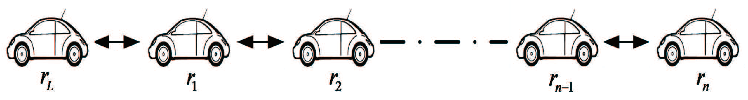
As shown in Figure 1, a string of autonomous vehicles move in a platoon, which includes a leader vehicle and n followers. Additionally, each follower regulates its motion according to the received information (e.g., position, velocity, acceleration, etc.) from its neighboring vehicles. The longitudinal dynamics of the i-th vehicle can be described by:
where is the mass of the i-th vehicle and and denote the position and velocity of the i-th vehicle, respectively. denotes the actuator output force of the i-th vehicle. In addition, describes the unknown driving resistance dynamics.
Assumption 1.
The desired velocity and its derivative are known and bounded.
Assumption 2.
The unknown driving resistance dynamics is smooth and bounded.
Definition 1.
The objective of this paper is to design a neural adaptive sliding-mode control algorithm for the whole vehicle platoon based on the CTH policy such that the following targets can be achieved:
- The position tracking error of each vehicle in the platoon is bounded, i.e., , where is a small positive constant and represents the position tracking error defined in (4);
- The string stability of the whole vehicle platoon can be guaranteed, i.e., ;
- The control algorithm uses few the information of vehicles.
Before proceeding to the design of the neural adaptive sliding-mode control algorithm, we give the following lemmas that will be used throughout the paper.
Lemma 1.
[39] There is a continuous function , and is bounded. Then, is bounded if the following inequality holds:
where and is a constant.
Lemma 2.
[40] RBF NNs can approximate online an unknown smooth function in the form of , where denotes the inputs of the neural network and q represents the dimension of neural network input. ; is the parameter vector and can be adjusted; m indicates the number of neurons. , where is the Gaussian function:
where and are the centers and widths of the Gaussian functions, respectively. RBF NNs can approximate to arbitrary accuracy by setting numerous hidden neurons:
the approximation error can be adjusted to be arbitrarily small by choosing ideal bounded weight vector. Additionally, is a small positive constant:
3. Main Results
In this section, two algorithms are developed, with the first algorithm in Section 3.1 requiring the information (position, velocity, acceleration) of neighboring vehicles, while the second algorithm in Section 3.2 requires only the position information of neighboring vehicles. In order to better present the control structure and the signal flow, a block diagram is provided for our proposed system in Figure 2.
3.1. Neural Adaptive Control Algorithm Using State Feedback
Firstly, RBF NNs are adopted to approximate online the and further construct the model:
where .
Then, the position tracking error for the i-th vehicle is defined as:
where is the standstill spacing and represents the constant time headway.
To overcome the degradation of system transient performance caused by large nonzero initial position tracking error, a modified position tracking error is defined as:
with:
where and is a positive constant. Thus, we have:
The importance of is that it can transform the nonzero initial position tracking error problem to a zero initial position tracking error problem. It is clear that converges to when converges to zero, where the rate of convergence can be determined by . Then, an integrated-sliding-mode surface is constructed as:
where is a positive parameter. It is clear that the convergence of the ISM surface can make be zero.
In order to guarantee the string stability of the whole vehicle platoon, the coupled sliding surface (CSS) is adopted to establish the relationship between the i-th and the ()-th vehicle:
where is a weighting factor.
It should be pointed out that is a nonexistent signal, so we set . Furthermore, we define the matrices and to depict the whole vehicle platoon. The relationship between and can be described as:
where:
The following lemma illustrates the same convergence of and .
Lemma 3.
[33] (Equivalence of the convergence of the CSS and each sliding surface toward zero): When converges to zero, also converges to zero at the same time.
Therefore, taking the time derivative of in (7), it yields:
where .
Particularly, we know that when . The time derivative of can be written as:
where .
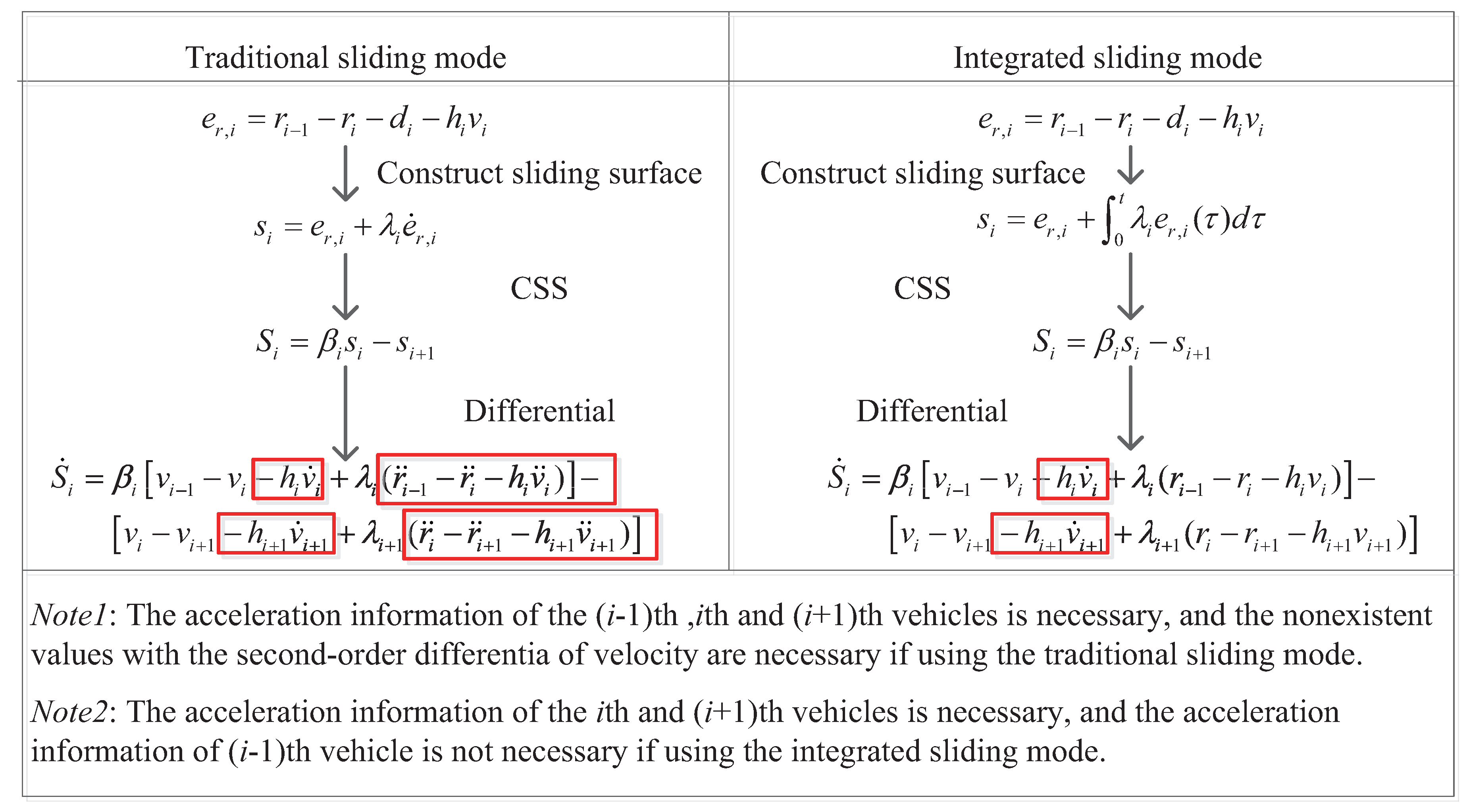
In Figure 3, the differences between traditional sliding-mode and integrated sliding-mode are shown to illustrate the advantages of the technique used in this paper.
Remark 1.
Comparing with the traditional sliding-mode approaches, the acceleration information of the followers is not needed using the ISM technique.
Remark 2.
The ISM technique can be employed to avoid the second-order differential of velocity caused by adopting the CTH policy.
Accordingly, the designed neural adaptive sliding-mode control algorithm for the whole vehicle platoon is given in the following theorem.
Theorem 1.
Consider the whole vehicle platoon described by (3) satisfying Assumptions 1 and 2. By using the following controller and adaptive estimation laws,
where and are control gains. and are the estimated values of and , respectively. and are small constants. , , and are small constants introduced in [40], which can prevent and from drifting to become very large. The following statements hold:
- The coefficients’ estimation error , and the signal are bounded, as well as converging to the following compact regions, respectively.where the detailed definition of φ and w is given later.
- The string stability of the whole vehicle platoon is guaranteed, i.e., .
Proof.
Consider the closed-loop dynamics of vehicles as:
where () is used to approximate the unknown driving resistance . and represent the estimated values of the optimal weight vector and estimation error , respectively.
Then, consider the following Lyapunov function candidate:
Taking the time derivative of (14), it yields:
Based on the Young’s inequality:
Then, Equation (15) can be written as:
Meanwhile, we define:
Then:
where and .
According to Lemma 1, we know that V is bounded. Additionally, with being the initial value of V when . Furthermore, we can know that the coefficients’ estimation error , and the signal converge to the following compact regions, respectively.
It is clear that the signal will be limited in a bounded compact region, and the bounds can be adjusted to an arbitrary small value by designing the ideal parameter . Furthermore, the position tracking error will be limited in a bounded region.
In addition, the string stability of the whole vehicle platoon can be proven by limiting the ratio, which takes into account the Laplace transform value of the i-th vehicle and its preceding vehicle. Since , we have:
Taking the Laplace transform of (21), it yields:
Let . We have:
Thus, if satisfies ; the transient position tracking errors from one vehicle to another vehicle cannot be enlarged, and the string stability of the whole vehicle platoon is guaranteed. ☐
3.2. Neural Adaptive Control Algorithm Using Output Feedback
In this section, an output feedback algorithm based on the higher order sliding-mode observer is presented to regulate the motion of vehicles.
Lemma 4.
[35] The velocity and acceleration of the i-th vehicle can be extracted from position based on the high-order sliding-mode observer:
where , and are parameters of the observer.
We assume that the velocity and acceleration of the i-th vehicle can be estimated from the position information with small observation errors:
where and represent the observed value of and , respectively. and denote the observation error with small positive constants and . Furthermore, we redefine the notations based on Section 3.1:
Accordingly, we further have the following theorem.
Theorem 2.
Consider the whole vehicle platoon described by (3). With the application of the controller and the adaptive update laws of the weight parameters of RBF NNs:
We have the following statements:
- The coefficients’ estimation error , and the signal are bounded and converge to the following compact sets:where the detailed definition of and is shown later.
- The string stability of the whole vehicle platoon is guaranteed, i.e., .
Proof.
The closed-loop dynamics of the vehicle platoon can be formulated as:
Consider the following Lyapunov function candidate:
Taking the time derivative of (30), it yields:
Next, we have:
Consider Young’s inequality in (16) and the facts that:
Thus, we have:
where:
Furthermore, we define:
Thus, it yields:
where and .
Using the same analysis as in Theorem 1, we can know that the signal and the coefficients’ estimation error and converge to the following compact sets:
Additionally, the string stability of the vehicle platoon is guaranteed by choosing . ☐
Remark 3.
By using the high-order sliding-mode observer, the velocity and acceleration are effectively obtained. The control objective for the vehicle platoon with only output feedback can be achieved, and the string stability can be guaranteed by the stability theorem.
Remark 4.
Both algorithms can guarantee the boundedness of the tracking error , and the coefficients’ estimation error , . However, the full state information (position, velocity and acceleration) is required in the first algorithm, while only position information is needed in the second algorithm.
4. Numerical Simulations
To evaluate the effectiveness and feasibility of the proposed platoon control approaches, numerical simulations are performed in this section. We apply the results to a seven-vehicle platoon.
4.1. Simulation Setup
The desired velocity curve is described as:
Actually, it has been pointed that the reasonable coefficients of spacing policy have significant effects on string stability for the whole vehicle platoon in [41]. We choose the coefficients in (4) with and according to the results in [41]. In addition, the initial positions and velocities of the vehicles in the platoon are designed as , and , .
The control parameters of the whole vehicle platoon are listed in Table 1:
4.2. Simulation Results
• Case 1: Vehicle platoon control using state feedback:
In this case, the algorithm in Section 3.1 is applied to control the vehicles such that the vehicles can move with the desired inter-vehicle distance.
The simulation results are shown in Figure 4. The tracking performances of velocities and velocity tracking errors are shown in Figure 4a,b, respectively. The position curves of vehicles and the inter-vehicle distance curves are shown in Figure 4c,d, which demonstrate that the vehicles in the platoon can move with safe inter-vehicle distance and avoid collisions. In addition, we can see that the inter-vehicle distance between two vehicles is related to the velocity of the vehicle from Figure 4d. It can be seen from Figure 4e that the string stability of the vehicle platoon is achieved, i.e., . The control input curves are shown in Figure 4f.
• Case 2: Vehicle platoon control using output feedback:
In this case, the algorithm in Theorem 2 is applied, and the parameters of the higher order sliding-mode observer are designed as , , .
From Figure 5a,b, it is clear that the convergence of the tracking performance of velocity is excellent, and the velocity estimation errors converge to a small region eventually. Meanwhile, the position curves and inter-vehicle distance curves are shown in Figure 5c,d, which are as good as those in Figure 4c,d. The position tracking error curves are shown in Figure 5e, and it is clear that . Meanwhile, it can be seen from Figure 5f that the observation errors of acceleration are limited to a small region.
It is worth pointing out that the convergence time of two algorithms is similar. From the results in Figure 4e and Figure 5e, we can see that the time consumptions of the two algorithms for the position tracking errors reaching the desired region are both about 50 s. However, only the position information is required in the second algorithm.
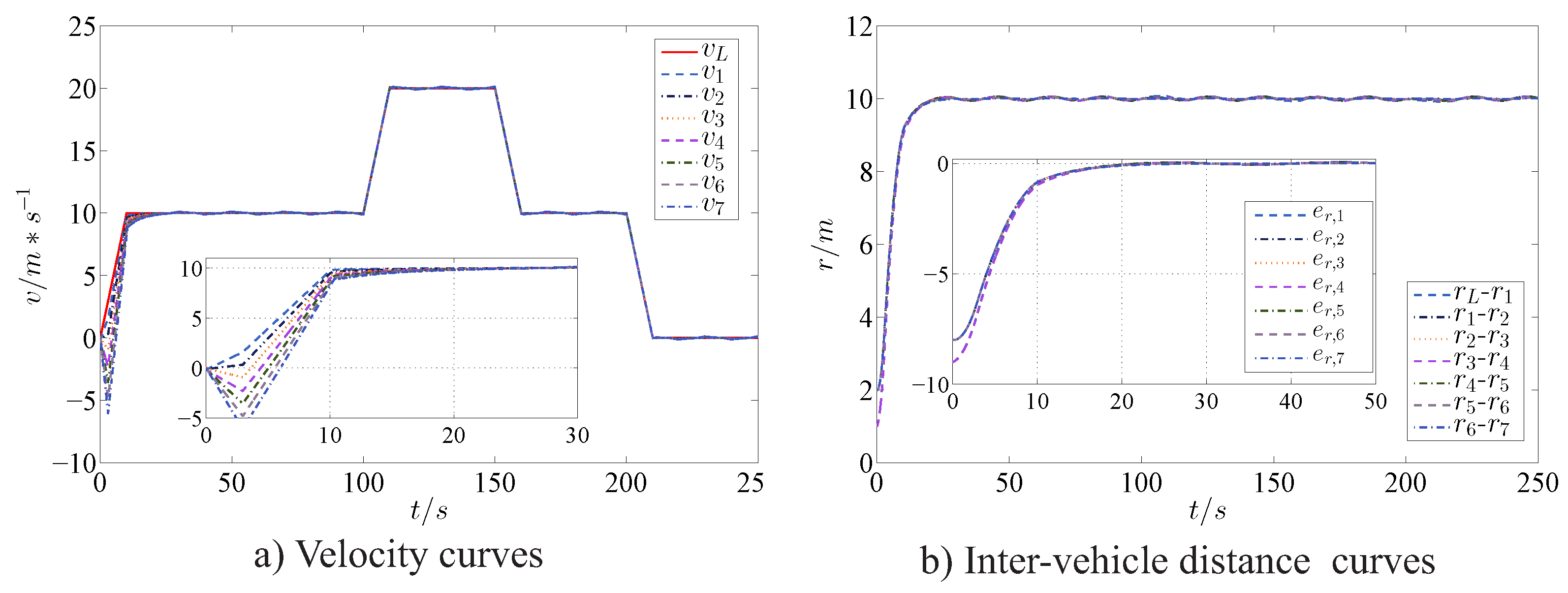
• Case 3: Comparative analysis:
In order to illustrate the advantages of the proposed algorithm compared with the method in [31], the algorithm in [31] is adopted to track the same desired velocity curve in (39).
Figure 6a,b shows the tracking performance of the control algorithm in [31]. It should be noted that the inter-vehicle distance converges to a constant value (10 m) in Figure 6b. Compared with the results in Figure 4d and Figure 5d (the inter-vehicle distance is related to the velocity of the vehicle, i.e., when m/s and 20 m/s, m and m, respectively), the control effects using the protocol in [31] seem too rigid. In addition, it should be pointed out that the algorithm in [31] achieves the control effects in Figure 6 by using state feedback. Above all, the proposed algorithm in this paper is more practical and pragmatic.
5. Conclusions
To simplify IFT, rationalize FG and reduce the communication load, this paper presents a novel output feedback control algorithm for the whole vehicle platoon based on a bidirectional communication strategy and the CTH policy. By using the ISM technique, a neural adaptive sliding-mode control algorithm is designed to ensure the desired inter-vehicle space. In order to decrease the communication load, a higher order sliding-mode observer is employed to estimate the information of velocity and acceleration, and an improved control protocol is further proposed for the vehicle platoon using only position information. The string stability of the vehicle platoon is proven through the stability theorem. Numerical simulations are provided to verify the feasibility and effectiveness of the proposed control methods.
Acknowledgments
This work is supported by the Key Science and Technology Program of Shaanxi Province (No. 2017JQ6060), China Postdoctoral Science Foundation (No. 2017M613030) and Fundamental Research Funds for the Central Universities of China (Nos. 310832171004, 310832163403, 310832101012).
Author Contributions
Maode Yan and Jiacheng Song designed the neural adaptive sliding-mode control algorithm and analyzed the string stability of the whole vehicle platoon. Jiacheng Song performed the numerical simulations and demonstrated the advantages over the traditional method. Lei Zuo and Panpan Yang analyzed the simulation data and revised the whole manuscript.
Conflicts of Interest
The authors declare no conflict of interest.
References
- Tsugawa, S.; Jeschke, S.; Shladover, S.E. A review of truck platooning projects for energy savings. IEEE Trans. Intell. Veh. 2016, 1, 68–77. [Google Scholar] [CrossRef]
- Englund, C.; Chen, L.; Ploeg, J.; Semsar-Kazerooni, E.; Voronov, A.; Bengtsson, H.H.; Didoff, J. The grand cooperative driving challenge 2016: Boosting the introduction of cooperative automated vehicles. IEEE Wirel. Commun. 2016, 23, 146–152. [Google Scholar] [CrossRef]
- Robinson, T.; Chan, E.; Coelingh, E. Operating platoons on public motorways: An introduction to the sartre platooning programme. In Proceedings of the 17th World Congress on Intelligent Transport Systems, Busan, Korean, 25–29 October 2010; pp. 1–11. [Google Scholar]
- Tsugawa, S.; Kato, S.; Aoki, K. An automated truck platoon for energy saving. In Proceedings of the IEEE/RSJ International Conference on Intelligent Robots and Systems (IROS), San Francisco, CA, USA, 25–30 September 2011; pp. 4109–4114. [Google Scholar]
- Besselink, B.; Johansson, K.H. String stability and a delay-based spacing policy for vehicle platoons subject to disturbances. IEEE Trans. Autom. Control 2017, 62, 4376–4391. [Google Scholar] [CrossRef]
- Lin, F.; Fardad, M.; Jovanović, M.R. Algorithms for leader selection in stochastically forced consensus networks. IEEE Trans. Autom. Control 2014, 59, 1789–1802. [Google Scholar] [CrossRef]
- Bernardo, M.D.; Salvi, A.; Santini, S. Distributed consensus strategy for platooning of vehicles in the presence of time-varying heterogeneous communication delays. IEEE Trans. Intell. Transp. Syst. 2015, 16, 102–112. [Google Scholar] [CrossRef]
- Ali, A.; Garcia, G.; Martinet, P. The flatbed platoon towing model for safe and dense platooning on highways. IEEE Intell. Transp. Syst. Mag. 2015, 7, 58–68. [Google Scholar] [CrossRef]
- Herman, I.; Dan, M.; Hurák, Z.; Šebek, M. Nonzero bound on fiedler eigenvalue causes exponential growth of H-Infinity norm of vehicular platoon. IEEE Trans. Autom. Control 2015, 60, 2248–2253. [Google Scholar] [CrossRef]
- Wu, Y.; Li, S.E.; Zheng, Y.; Hedrick, J.K. Distributed sliding mode control for multi-vehicle systems with positive definite topologies. In Proceedings of the IEEE 55th Conference on Decision and Control, Las Vegas, NV, USA, 12–14 December 2016; pp. 5213–5219. [Google Scholar]
- Xiao, L.; Gao, F. Practical string stability of platoon of adaptive cruise control vehicles. IEEE Trans. Intell. Transp. Syst. 2011, 12, 1184–1194. [Google Scholar] [CrossRef]
- Dunbar, W.B.; Caveney, D.S. Distributed receding horizon control of vehicle platoons: Stability and string stability. IEEE Trans. Autom. Control 2012, 57, 620–633. [Google Scholar] [CrossRef]
- Hao, H.; Barooah, P. On achieving size-independent stability margin of vehicular lattice formations with distributed control. IEEE Trans. Autom. Control 2011, 57, 2688–2694. [Google Scholar] [CrossRef]
- Zheng, Y.; Li, S.E.; Wang, J.; Cao, D.; Li, K. Stability and scalability of homogeneous vehicular platoon: Study on the influence of information flow topologies. IEEE Trans. Intell. Transp. Syst. 2015, 17, 14–26. [Google Scholar] [CrossRef]
- Zheng, Y.; Li, S.E.; Li, K.; Wang, L.Y. Stability margin improvement of vehicular platoon considering undirected topology and asymmetric Control. IEEE Trans. Control Syst. Technol. 2016, 24, 1253–1265. [Google Scholar] [CrossRef]
- Hao, H.; Barooah, P. Stability and robustness of large platoons of vehicles with double-integrator models and nearest neighbor interaction. Int. J. Robust Nonlinear Control 2013, 23, 2097–2122. [Google Scholar] [CrossRef]
- Kianfar, R.; Falcone, P.; Fredriksson, J. A receding horizon approach to string stable cooperative adaptive cruise control. In Proceedings of the International IEEE Conference on Intelligent Transportation Systems, Washington, DC, USA, 5–7 October 2011; pp. 734–739. [Google Scholar]
- Qin, J.; Ma, Q.; Shi, Y.; Kang, Y. On group synchronization for interacting clusters of heterogeneous systems. IEEE Trans. Cybern. 2017, 47, 4122–4133. [Google Scholar] [CrossRef] [PubMed]
- Mu, J.; Yan, X.G.; Spurgeon, S.K. Decentralised sliding mode control for a class of nonlinear interconnected systems. In Proceedings of the American Control Conference, Chicago, IL, USA, 1–3 July 2015; pp. 5170–5175. [Google Scholar]
- Shi, Y.; Shen, C.; Fang, H.; Li, H. Advanced control in marine mechatronic systems: A survey. IEEE/ASME Trans. Mechatronics 2017, 22, 1121–1131. [Google Scholar] [CrossRef]
- Tangerman, F.M.; Veerman, J.J.P.; Stosic, B.D. Asymmetric decentralized flocks. IEEE Trans. Autom. Control 2012, 57, 2844–2853. [Google Scholar] [CrossRef]
- Mu, B.; Zhang, k.; Shi, Y. Integral sliding mode flight controller design for a quadrotor and the application in a heterogeneous multi-agent system. IEEE Trans. Ind. Electron. 2017, 64, 9389–9398. [Google Scholar] [CrossRef]
- Alam, A.; Gattami, A.; Johansson, K.H.; Tomlin, C.J. Guaranteeing safety for heavy duty vehicle platooning: Safe set computations and experimental evaluations. Control Eng. Pract. 2014, 24, 33–41. [Google Scholar] [CrossRef]
- Mu, B.; Shi, Y.; Chen, J.; Chang, Y. Design and implementation of non-uniform sampling cooperative control on a group of two-wheeled mobile robots. IEEE Trans. Ind. Electron. 2017, 64, 5035–5044. [Google Scholar] [CrossRef]
- Guo, G.; Yue, W. Autonomous platoon control allowing range-limited sensors. IEEE Trans. Veh. Technol. 2012, 61, 2901–2912. [Google Scholar] [CrossRef]
- Qin, J.; Ma, Q.; Shi, Y.; Wang, L. Recent advances in consensus of multi-agent systems: A brief survey. IEEE Trans. Ind. Electron. 2017, 64, 4972–4983. [Google Scholar] [CrossRef]
- Ploeg, J.; Wouw, N.V.D.; Nijmeijer, H. Lp string stability of cascaded systems: Application to vehicle platooning. IEEE Trans. Control Syst. Technol. 2014, 22, 786–793. [Google Scholar] [CrossRef]
- Milanes, V.; Shladover, S.E.; Spring, J.; Nowakowski, C.; Kawazoe, H.; Nakamura, M. Cooperative adaptive cruise control in real traffic situations. IEEE Trans. Intell. Transp. Syst. 2014, 15, 296–305. [Google Scholar] [CrossRef]
- Öncü, S.; Ploeg, J.; Wouw, N.V.D.; Nijmeijer, H. Cooperative adaptive cruise control: Network-aware analysis of string stability. IEEE Trans. Intell. Transp. Syst. 2014, 15, 1527–1537. [Google Scholar] [CrossRef]
- Bernardo, M.D.; Falcone, P.; Salvi, A.; Santini, S. Design, analysis, and experimental validation of a distributed protocol for platooning in the presence of time-varying heterogeneous delays. IEEE Trans. Control Syst. Technol. 2016, 24, 413–427. [Google Scholar] [CrossRef]
- Kwon, J.W.; Chwa, D. Adaptive bidirectional platoon control using a coupled sliding mode control method. IEEE Trans. Intell. Transp. Syst. 2014, 15, 2040–2048. [Google Scholar] [CrossRef]
- Guo, X.; Wang, J.; Liao, F.; Teo, R.S.H. Distributed adaptive sliding mode control strategy for vehicle-following systems with nonlinear acceleration uncertainties. IEEE Trans. Veh. Technol. 2017, 66, 981–991. [Google Scholar] [CrossRef]
- Guo, X.; Wang, J.; Liao, F.; Teo, R.S.H. Distributed adaptive integrated-sliding-mode controller synthesis for string stability of vehicle platoons. IEEE Trans. Intell. Transp. Syst. 2016, 17, 2419–2429. [Google Scholar] [CrossRef]
- Yan, X.G.; Spurgeon, S.K.; Orlov, Y. Output feedback control synthesis for non-linear time-delay systems using a sliding-mode observer. IMA J. Math. Control Inf. 2014, 31, 501–508. [Google Scholar] [CrossRef]
- Levant, A. Higher-order sliding modes, differentiation and output-feedback control. Int. J. Control 2003, 76, 924–941. [Google Scholar] [CrossRef]
- Levant, A. Universal output-feedback siso controller. IFAC Proc. Vol. 2002, 35, 221–226. [Google Scholar] [CrossRef]
- Bayar, B.; Sajadi-Alamdari, S.A.; Viti, F.; Voos, H. Impact of different spacing policies for adaptive cruise control on traffic and energy consumption of electric vehicles. In Proceedings of the 24th Mediterranean Conference on Control and Automation, Athens, Greece, 21–24 June 2016; pp. 1349–1354. [Google Scholar]
- Klinge, S.; Middleton, R.H. Time headway requirements for string stability of homogeneous linear unidirectionally connected systems. In Proceedings of the IEEE Conference on Decision and Control, Shanghai, China, 15–18 December 2009; pp. 1992–1997. [Google Scholar]
- Gao, S.G.; Dong, H.R.; Ning, B.; Clive, R.; Chen, L.; Sun, X.B. Cooperative adaptive bidirectional control of a train platoon for efficient utility and string stability. Chin. Phys. B 2015, 24, 161–170. [Google Scholar] [CrossRef]
- Gao, S.G.; Dong, H.R.; Ning, B.; Chen, Y.; Sun, X. Adaptive fault-tolerant automatic train operation using RBF neural networks. Neural Comput. Appl. 2015, 26, 141–149. [Google Scholar] [CrossRef]
- Yanakiev, D.; Kanellakopoulos, I. Nonlinear spacing policies for automated heavy-duty vehicles. IEEE Trans. Veh. Technol. 1998, 47, 1365–1377. [Google Scholar] [CrossRef]
Figure 1.
Topological structure of the vehicle platoon.

Figure 2.
The control system architecture and the signal flow in the control system.
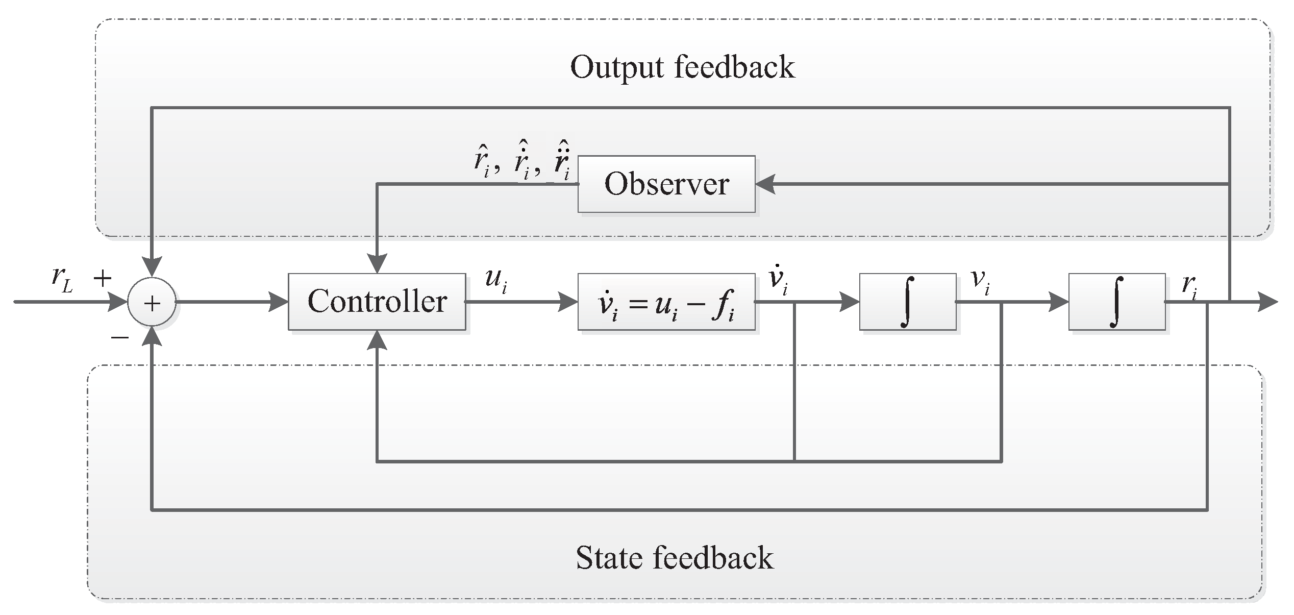
Figure 3.
The difference between traditional sliding mode and integrated sliding mode.

Figure 4.
Vehicles’ performance using full state information: (a) Velocity of each vehicle; (b) Velocity tracking error; (c) Position curves; (d) Inter-vehicle distance between two consecutive vehicles; (e) Position tracking error; (f) Control input of each vehicle.
Figure 4.
Vehicles’ performance using full state information: (a) Velocity of each vehicle; (b) Velocity tracking error; (c) Position curves; (d) Inter-vehicle distance between two consecutive vehicles; (e) Position tracking error; (f) Control input of each vehicle.
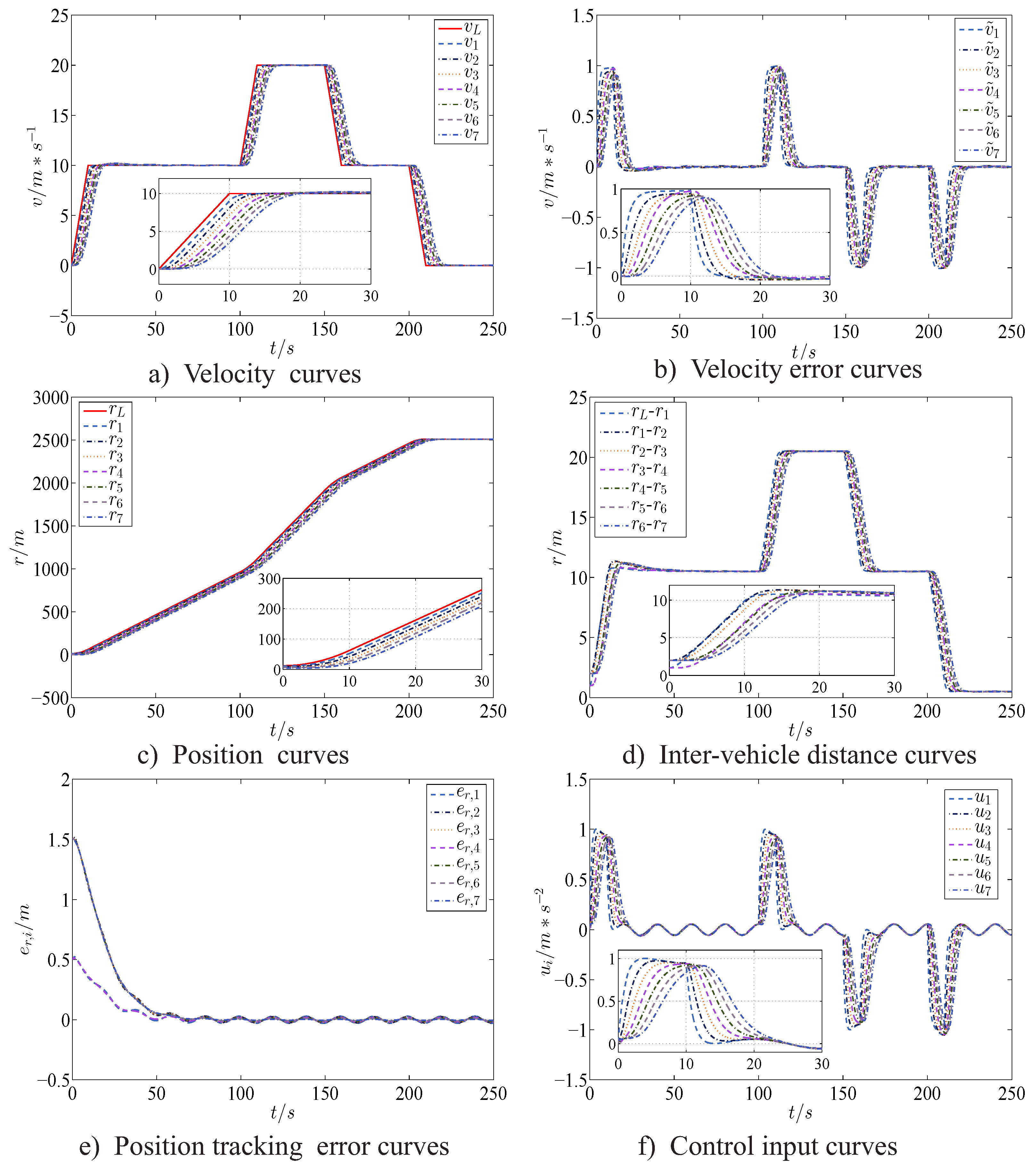
Figure 5.
Vehicles’ performance using position information: (a) Velocity of each vehicle; (b) Velocity estimation error; (c) Position curves; (d) Inter-vehicle distance between two consecutive vehicles; (e) Position tracking error; (f) Acceleration estimation error.
Figure 5.
Vehicles’ performance using position information: (a) Velocity of each vehicle; (b) Velocity estimation error; (c) Position curves; (d) Inter-vehicle distance between two consecutive vehicles; (e) Position tracking error; (f) Acceleration estimation error.
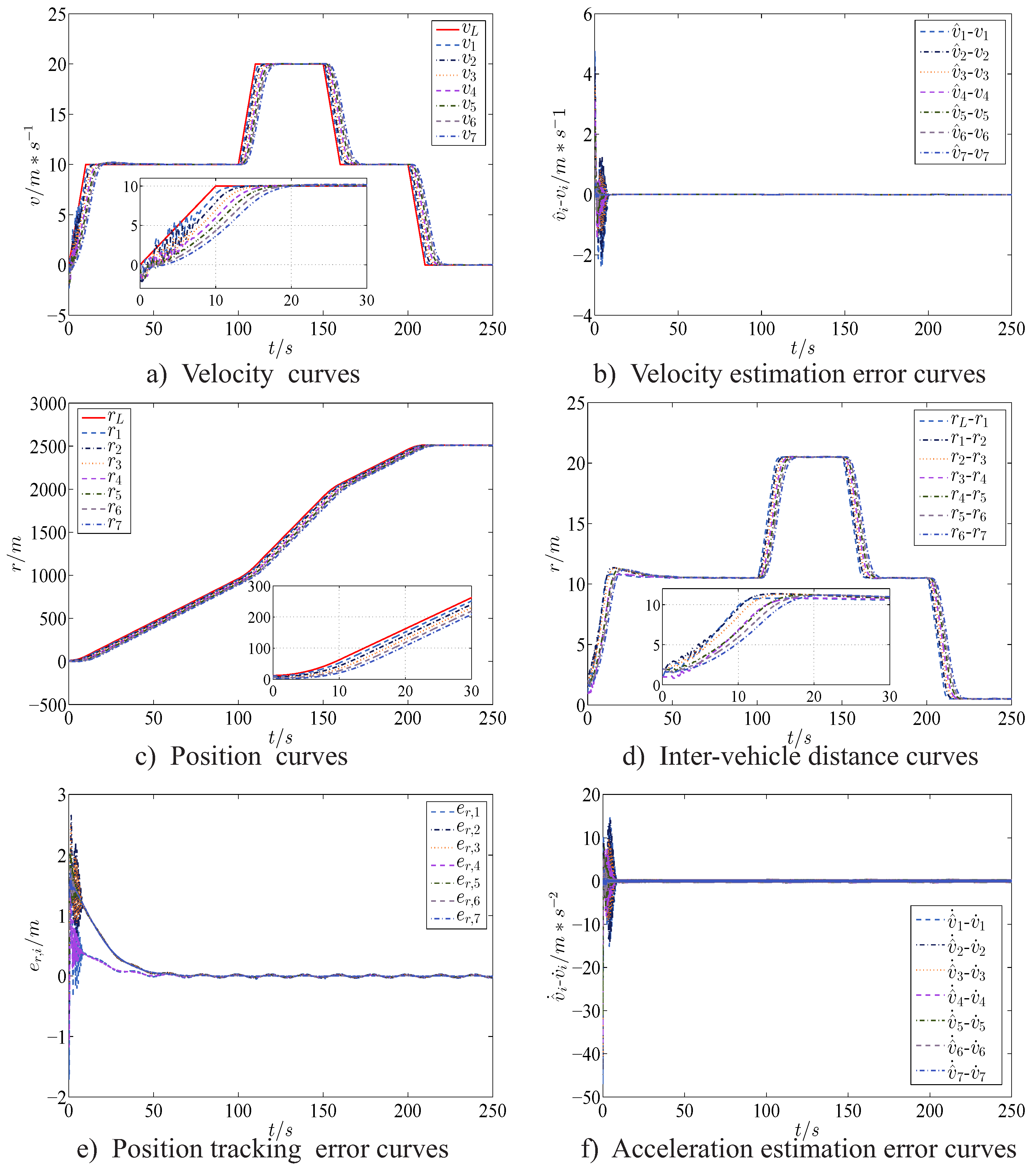
Figure 6.
Vehicles’ performance using a similar method as in [31]: (a) Velocity of each vehicle; (b) Inter-vehicle distance between two consecutive vehicles.
Figure 6.
Vehicles’ performance using a similar method as in [31]: (a) Velocity of each vehicle; (b) Inter-vehicle distance between two consecutive vehicles.

Table 1.
Control parameters.
| 10 | 1 | 10 | 10 | 5 | 5 |
© 2017 by the authors. Licensee MDPI, Basel, Switzerland. This article is an open access article distributed under the terms and conditions of the Creative Commons Attribution (CC BY) license (http://creativecommons.org/licenses/by/4.0/).
Share and Cite
MDPI and ACS Style
Yan, M.; Song, J.; Zuo, L.; Yang, P. Neural Adaptive Sliding-Mode Control of a Vehicle Platoon Using Output Feedback. Energies 2017, 10, 1906. https://doi.org/10.3390/en10111906
AMA Style
Yan M, Song J, Zuo L, Yang P. Neural Adaptive Sliding-Mode Control of a Vehicle Platoon Using Output Feedback. Energies. 2017; 10(11):1906. https://doi.org/10.3390/en10111906
Chicago/Turabian StyleYan, Maode, Jiacheng Song, Lei Zuo, and Panpan Yang. 2017. "Neural Adaptive Sliding-Mode Control of a Vehicle Platoon Using Output Feedback" Energies 10, no. 11: 1906. https://doi.org/10.3390/en10111906
Note that from the first issue of 2016, this journal uses article numbers instead of page numbers. See further details here.