An Interval Fuzzy-Stochastic Chance-Constrained Programming Based Energy-Water Nexus Model for Planning Electric Power Systems

1
Department of Environmental Engineering, Xiamen University of Technology, Xiamen 361024, China
2
School of Environment, Beijing Normal University, Beijing 100875, China
3
Institute for Energy, Environment and Sustainability Research, University of Regina, Regina, SK S4S 0A2, Canada
4
Sino-Canada Energy and Environmental Research Center, North China Electric Power University, Beijing 102206, China
5
State Grid Henan Economic Research Institute; No. 87 South Songshan Road, Zhengzhou 450052, China
*
Author to whom correspondence should be addressed.
Energies 2017, 10(11), 1914; https://doi.org/10.3390/en10111914
Submission received: 1 October 2017
/
Revised: 5 November 2017
/
Accepted: 13 November 2017
/
Published: 20 November 2017
Abstract
:In this study, an interval fuzzy-stochastic chance-constrained programming based energy-water nexus (IFSCP-WEN) model is developed for planning electric power system (EPS). The IFSCP-WEN model can tackle uncertainties expressed as possibility and probability distributions, as well as interval values. Different credibility (i.e., γ) levels and probability (i.e., qi) levels are set to reflect relationships among water supply, electricity generation, system cost, and constraint-violation risk. Results reveal that different γ and qi levels can lead to a changed system cost, imported electricity, electricity generation, and water supply. Results also disclose that the study EPS would tend to the transition from coal-dominated into clean energy-dominated. Gas-fired would be the main electric utility to supply electricity at the end of the planning horizon, occupying [28.47, 30.34]% (where 28.47% and 30.34% present the lower bound and the upper bound of interval value, respectively) of the total electricity generation. Correspondingly, water allocated to gas-fired would reach the highest, occupying [33.92, 34.72]% of total water supply. Surface water would be the main water source, accounting for more than [40.96, 43.44]% of the total water supply. The ratio of recycled water to total water supply would increase by about [11.37, 14.85]%. Results of the IFSCP-WEN model present its potential for sustainable EPS planning by co-optimizing energy and water resources.
1. Introduction
It is predicted that the electricity demand will increase about 34.51% in 2035 due to population growth, economic development, industrialization, and urbanization throughout the world [1,2]. It is essential to consume more energy resources to satisfy the rising electricity demand. In fact, energy security is highly dependent on water availability since the processes of extracting and refining fossil fuels, electricity generation, transportation, and storage demand vast amounts of water; in turn, water extraction, conveyance, treatment, and disposal require high energy use [3,4]. The interdependence between energy and water resources is commonly defined as the energy-water nexus. For electric power systems (EPS), water is supplied to produce hydro power and cool systems (open-loop, closed-loop and dry) in thermoelectric power plants (e.g., coal, natural gas, and nuclear), representing a significant branch of the energy-water nexus [5]. It is of great significance to effectively plan EPS based on the energy-water nexus due to the increased energy and water demands as well as the decreased energy and water availabilities [6].
Many researchers have studied analyzing the energy-water nexus to involve energy and water in the same systematic management problem. In 1994, Gleick used a full-scale Life cycle assessment (LCA) to explain and quantify the water intensity of energy resource extraction in the processes of power generation as well as the energy intensity of the water extraction during conveyance, treatment, distribution, and end use [7,8]. Recently, more researchers attempted to explore the energy-water nexus based on optimization techniques from a system point of view [9,10,11,12]. For example, Bazilian et al. [13] presented a modeling framework that specifically addressed the energy-water nexus from a developing country perspective, and could thus serve to inform more effective national policies and regulations. Dubreuil et al. [14] advanced an energy optimization model by incorporating a dedicated water module to joint optimize water and energy allocations, to assess the chances of reused water and nonconventional water resources in water scarce regions, as well as to analyze the variations in electricity demand when taking water into account. Van et al. [15] explored the impact of climate change on the European electricity generation, in which water availability for hydropower generation and cooling water usage for thermoelectric power production were analyzed. Liu et al. [16] employed an integrated model to assess future electricity generation and consumption as well as the related water withdrawals and consumption in the U.S under different scenarios (associated with the generation fuel portfolio, cooling technology mix, and their associated water use intensities). Lubega and Farid [17] developed a quantitative engineering system model to optimize the energy-water nexus systems, including electricity generation, engineered water supply, and wastewater management. Santhosh et al. [18] contributed a production cost co-optimization method for assessing the impact of storage facility capacity and ramping capabilities on the supply side economic dispatch of the energy-water nexus. Yang and Chen [8] proposed an energy-water nexus analysis framework for wind power generation systems, where energy for water supply and water for electricity generation were investigated. Gjorgiev and Giovanni [19] focused on the effects of water policy constraints on electric power generation in changing climate conditions, in which severe drought conditions leading to small river flows and high water temperatures were analyzed, and the limitations on the energy conversion at the thermal plant stemming from the water policies were quantified.
In fact, various uncertainties (e.g., electricity demand/supply, conversion efficiency, resources availability, and economic data) and their interactions are unavoidable to be taken into account since they may intensify the complexities in the planning procedures [20]. Conventional research efforts have difficulties in addressing uncertainties and their interactions. Previously, a number of inexact optimization models were developed for handling uncertainties and their interactions (in water management and EPS planning problems) through fuzzy, stochastic, and interval programming approaches [21,22,23,24,25,26,27,28,29,30]. Among them, the interval fuzzy credibility-constrained programming (IFCP) method is a computationally efficient hybrid approach that can tackle epistemic uncertainties presented in the form of fuzzy membership functions and intervals. It has been applied to water management to demonstrate its capability [22,31]; no applications of it to reflect and address the uncertainties associated with EPS management have been reported. On the other hand, the IFCP method is not effective for problems where uncertainties can only be expressed as random variables with known probability distributions. Chance-constrained programming (CCP) can handle randomness by allowing a set of related constraints to have finite probability of being violated [32]. By introducing the CCP into the IFCP framework, an interval fuzzy-stochastic chance-constrained programming (IFSCP) method can be formulated to cope with multiple uncertainties.
Therefore, this study aims to develop an interval fuzzy-stochastic chance-constrained programming based energy-water nexus (IFSCP-WEN) model for planning an electric power system. The detailed tasks entail: (1) integrating the CCP into the IFCP framework to formulate the IFSCP method; (2) dealing with uncertainties expressed in terms of possibility distributions, interval values, and probability distributions; (3) analyzing optimization results of electricity generation, water supply, capacity expansion, and pollution control under a variety of constraint-violation levels. The results can be helpful for decision makers to gain insight into the tradeoffs between water supply and electricity generation as well as the system cost and the constraint-violation risk.
2. Study System
2.1. Problem Statement
In this study, five main components are considered in an EPS. These include (i) the energy supply sector, which provides energy resources with different diverse resources; (ii) the electricity generation sector, which contains various electricity generation technologies as well as capacity expansion and imported electricity options with varied economic, environmental, and technological performance; (iii) the water supply sector, which supplies water to produce hydro power and cool systems (open-loop, closed-loop and dry); (iv) the electricity demand sector, which involves certain kinds of demand side technologies to fulfill the demand of many end users and is determined by varying socio-economic, geographical, technological, and environmental conditions; (v) the pollution mitigation sector, which regulates pollution mitigation policies [33]. Decision makers are often responsible for allocating electricity from multiple electric utilities to multiple end users over a planning horizon.
The decision maker can formulate the problem as minimizing the system cost by identifying sound schedules of imported electricity, electricity generation, water supply, and capacity expansion. A range of constraints are presented as a set of linear inequalities for defining the relationship between electricity and water supplies, resources availabilities, electricity and water demands, and environmental restrictions. In fact, such a system is complicated due to the following: (1) management of energy and water sources has complex interactions with many other components, such as environment, ecosystem, and socio-economy; (2) complex relationships between different activities/services (e.g., imported electricity, electricity generation, capacity expansion, water supply, and pollution reduction) and their related economic and environmental implications. In addition, inherent uncertainties and intensive interactions (which are subject to temporal and spatial variations) exist among various factors [34]. They need to be effectively incorporated into the planning processes and the obtained decision alternatives. For example, energy demands may be affected by a number of factors such as population growth rate, economy development strategy, electricity demand, and supply policy; electricity generation may change with varied resource availabilities; costs which are related to the facilities/techniques may fluctuate with market conditions. Effective EPS planning should take these complications and uncertainties into account
2.2. System Description
Consider a representative EPS where electricity is supplied to multiple end users over a six-year planning horizon (with each having two years). Multiple energy resources include coal, natural gas, water, nuclear fuel, wind, and solar energies are supplied, thus six electric utilities (i.e., coal-fired, gas-fired, hydro, nuclear, wind, and solar power) are available for installation to meet the electricity demand in each period. Surface water, groundwater, and recycled water are identified as water supply sources since the process of generating electricity needs a large amount of water. They supply water to coal-fired, gas-fired, hydropower, and nuclear power utilities (wind and solar power are not considered due to their low water demands). Generally, electricity demand rises with time due to economy development and population growth; therefore, the decision makers are forced to expand the existing electric power utilities or import electricity to fulfil the increasing demand. The expansions are restrained by water and energy availabilities, cost of technologies, conversion efficiencies, capital investments, operation costs, and environmental concerns, while imported electricity is mainly determined by the importing cost. Moreover, the interrelationship between energy and water can greatly affect the decision making processes. For example, different electricity generation technologies have diverse water demands and costs of supplying electricity (for extracting, treating, and delivering water); different water sources correspond to different electricity demands and costs of allocating water (to different electric utilities). It is necessary to consider the energy-water nexus when planning the EPS.
3. Development of IFSCP-WEN
3.1. IFSCP Method
First, an interval fuzzy credibility-constraint programming (IFCP) method is formulated through coupling fuzzy credibility-constrained programming (FCP) with interval-parameter programming (IPP). The IFCP method is effective in handling uncertainties expressed as interval values and possibility distributions, which can be presented as follows [31]:
subject to:
where is the vector of non-fuzzy decision variables; , , and are the right-hand side coefficients; denotes the credibility level if a fuzzy event in ; and denote the predetermined credibility levels (managers prefer that it be satisfied under a high credibility level, with and ); and are the coefficients that can be described as fuzzy membership functions. is a trapezoidal or triangular fuzzy variable that can be expressed as of crisp numbers with [35]. The expected values of can be calculated as , leading to:
For the credibility constraints, assume that is fully determined by the triplet of crisp numbers with . Through deducing the deterministic equivalent of credibility constraints, Equations (1c) and (1d) can be converted as follows [36]:
The main limitation of IFCP lies in its difficulty in reflecting random features of constraints. Consequently, the chance-constrained programming (CCP) technique can be incorporated within the IFCP framework, leading to an interval fuzzy-stochastic chance-constrained programming (IFSCP) method as follows:
subject to:
where is the probability of violating constraint i. The IFSCP can be solved based on an interactive algorithm [37]. The detailed solution method is listed in Appendix A.
3.2. IFSCP-WEN Modeling Formulation
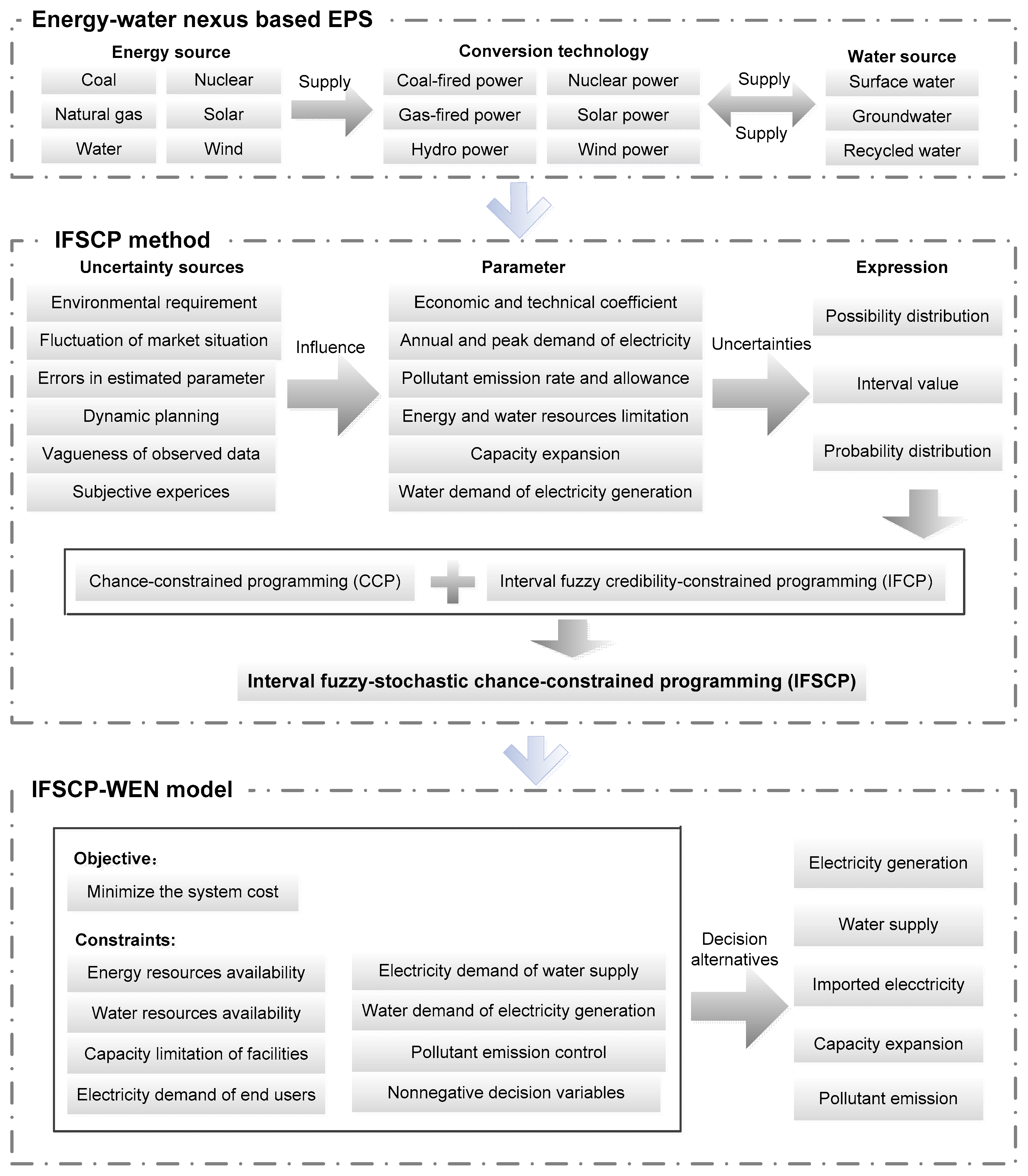
Based on the IFSCP method, an interval fuzzy-stochastic chance-constrained programming based energy-water nexus (IFSCP-WEN) model can be developed for planning the EPS. Figure 1 describes the framework of the IFSCP-WEN model. The objective of the IFSCP-WEN model is to minimize the system cost, including the cost for purchasing energy resources, the cost for importing electricity, the cost of electricity generation, the cost for capacity expansion, the cost of water supply, and the cost of pollution mitigation. In detail, the proposed IFSCP-WEN model can be formulated as follows:
Subject to:
- (1)
- Energy resources availability:
- (2)
- Water resources availability:
- (3)
- Capacity limitation of facilities:
- (4)
- Electricity demand of end users:
- (5)
- Electricity demand for water supply:
- (6)
- Water demand for electricity generation:
- (7)
- Pollutant emission control constraints:
- (8)
- Capacity expansion constraints:
- (9)
- Non-negative constraint:
In this study, it is assumed that credibility level γ = λ and six levels are taken into account (i.e., 0.55, 0.65, 0.75, 0.85, 0.95, and 0.99). Appendix B presents the nomenclatures for the parameters and variables.
3.3. Data Analysis
In this study, the imprecise inputs are presented as possibility distributions, probability distributions, and interval numbers. Table 1 provides the costs of electricity generation (including fixed and variable costs) which are presented as possibility distributions [37]. The costs are subjected to a range of factors (i.e., energy price and quality, labor fee, and operation condition); furthermore, activities for electricity generation may contain numerous capitals from multiple sources, resulting in varied interest rates. Summarily, coal and natural gas-fired electricity utilities correspond to lower operation cost; hydro, wind, and solar electricity utilities are associated with higher cost since their availability and stability concerns the authorities; nuclear electricity is also produced at a high cost partly due to the high investment for guaranteeing safety. Table 2 lists energy-water nexus related data [38]. Summarily, energy-water nexus includes: (i) water for electricity generation (mainly for cooling systems); (ii) groundwater and surface water extractions, bulk water (surface water groundwater, and recycled water) transfers, retail water distribution, wastewater collection, and wastewater treatment all need a certain amount of electricity [39]. The related data are expressed as possibility distributions due to imprecise information and subjective estimations. Besides, various factors could affect electricity demand (i.e., annual- and peak-demand) such as population growth, socio-economic development, changing weather condition, and the stochastic individual usage, resulting in the presentation of the electricity demand being a probability distribution [40]. Table 3 shows the electricity demand under three levels of violating electricity demand ( = 0.01, 0.05, and 0.10) [41].
4. Result Analysis and Discussion
4.1. System Cost
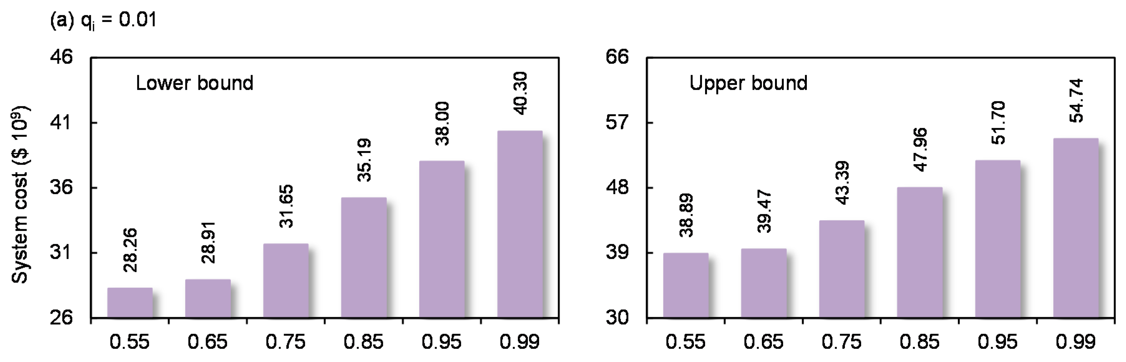
Figure 2 shows the system cost under each credibility (i.e., γ) level and probability (i.e., ) level, where the system costs would increase with raised γ levels and decrease with raised levels. For example, when = 0.01, the system cost would be $[28.26, 38.89] × 109 under γ = 0.55; in comparison, it would be $[40.30, 54.74] × 109 under γ = 0.99. This is because higher γ levels correspond to a stricter allowable magnitude of violating fuzzy constraints, leading to higher costs to alleviate the constraint-violation risks. When γ = 0.65, the system cost would be $[21.74, 30.65] × 109 under = 0.05, while it would be $[16.38, 23.12] × 109 under = 0.10. This is due to the fact that higher levels are related to lower electricity demands and thus result in lower system costs. In summary, the decision associated with a higher γ level and a lower level would carry increased reliability in fulfilling the system requirements and a higher system cost; a strong desire to reduce the system cost would entail a raised risk of violating the credibility- and chance-constraints.
4.2. Electricity and Water Supply Patterns
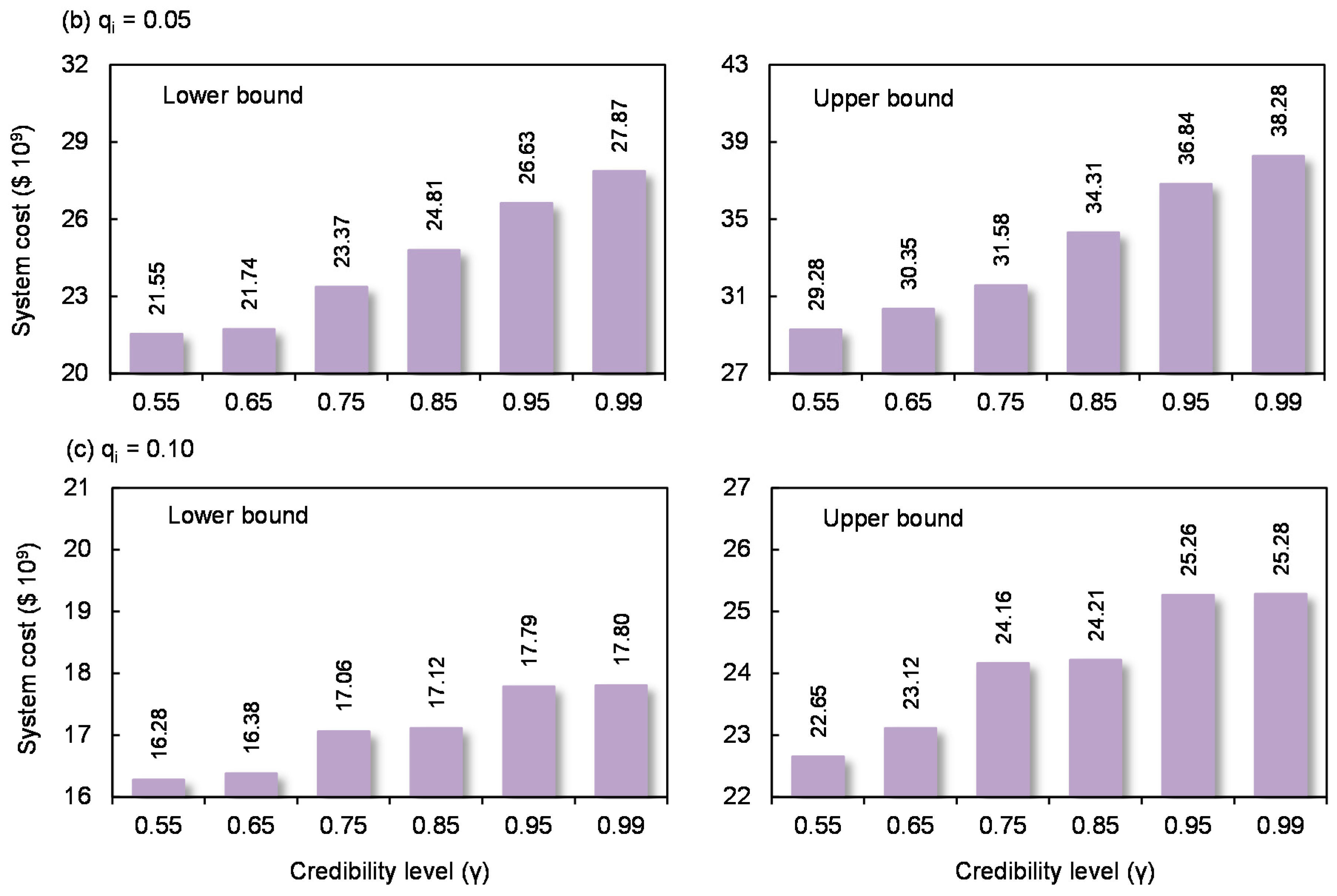
The effects on the electricity (i.e., imported electricity and electricity generation) and water supply patterns under each and γ levels are shown in Figure 3. It is demonstrated that the imported electricity, electricity generation, and water supply would vary with γ and levels. Generally, imported electricity would ascend with raised γ levels and descend with raised levels; electricity generation and water supply would decrease with raised γ and levels. For example, when γ = 0.55, the amounts of imported electricity, electricity generation, and water supply would respectively be [9.95, 12.45] × 103 GWh, [60.06, 63.53] × 103 GWh, and [134.98, 189.81] × 103 m3 in period 1 under = 0.01, while they would respectively be [7.21, 11.27] × 103 GWh, [47.21, 52.29] × 103 GWh, and [129.15, 165.63] × 103 m3 under = 0.10. When = 0.05, the amounts of imported electricity, electricity generation, and water supply would be [18.74, 20.01] × 103 GWh, [54.14, 56.11] × 103 GWh, and [149.28, 196.49] × 103 m3 in period 2 under γ = 0.65; in comparison, they would respectively be [21.04, 22.94] × 103 GWh, [51.57, 53.73] × 103 GWh, and [139.03, 157.17] × 103 m3 under γ = 0.95. This is because decision makers with a lower γ level possess a risk-neutral attitude (with a loose allowable magnitude of violating available resources and allowable pollutant emission related constraints); contrarily, decision makers with a higher γ level own a risk-averse attitude (leading to less electricity generation and water supply). Thus, more electricity would be imported to compensate for the growth of electricity shortage. Moreover, higher levels are associated with lower electricity demands and thus result in a decline in imported electricity, electricity generation, and water supply.
4.3. Distribution of Electricity Generation
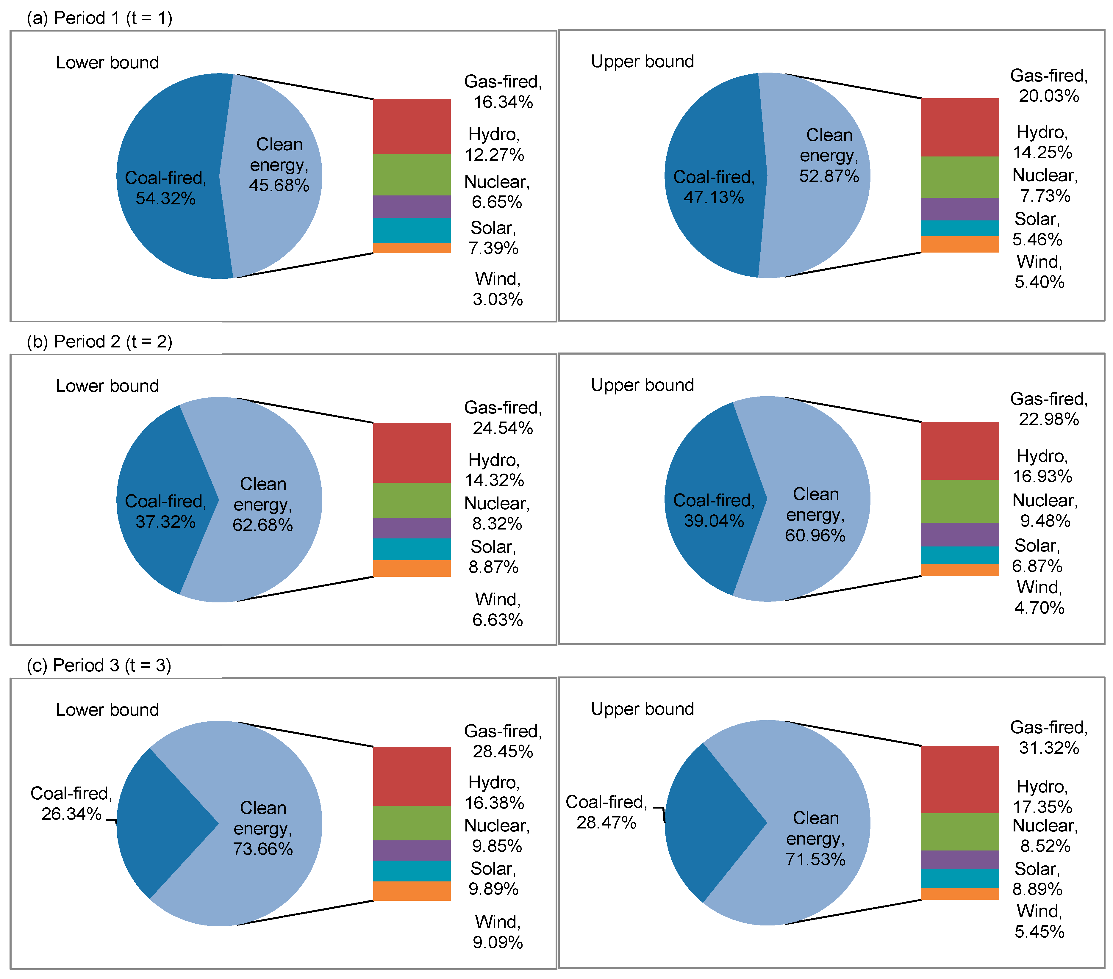
Figure 4 displays the distribution of electricity generation in each period. It is obvious that coal-fired and gas-fired would be the dominant electricity conversion technologies in the EPS. Specifically, the ratio of coal-fired power to total generation would drop with time and gas-fired power would increase with time. For example, coal-fired and gas-fired power would respectively account for [47.13, 54.32]% and [16.34, 20.03]% of the total electricity generation in period 1, while coal-fired and gas-fired power would respectively occupy [22.54, 24.32]% and [28.47, 30.34]% of the total electricity generation in period 3. The decreased use of raw material for coal-fired power would be ascribed to its high pollutant emission rate and resource shortage; in comparison, gas-fired is a technology with high electricity generation efficiency and low emission rate. Generally, the energy supply structure would tend to the transition from coal-dominated into clean energy-dominated due to the aim of sustainable development (i.e., clean burning, energy saving and emission reduction). In addition, hydro would also account for a high proportion of electricity generation due to the superiority of large capacity and highly available water resources. It would occupy [12.27, 14.25]%, [14.32, 16.93]% and [16.38, 17.35]% of the total electricity generation in periods 1–3, respectively. In terms of other energy sources (i.e., nuclear, solar, and wind), they would have small contributions to electricity generation due to their limited available resources (including water resources), low service time and/or small capacity. Under such a generation pattern, the capacity expansion of clean energy would be inevitable to meet a rapid increment. It is indicated that capacity expansion is focused on gas-fired. Other electric utilities are too small, so that this is neglected in the results analysis.
4.4. Water Allocation for Electricity Generation
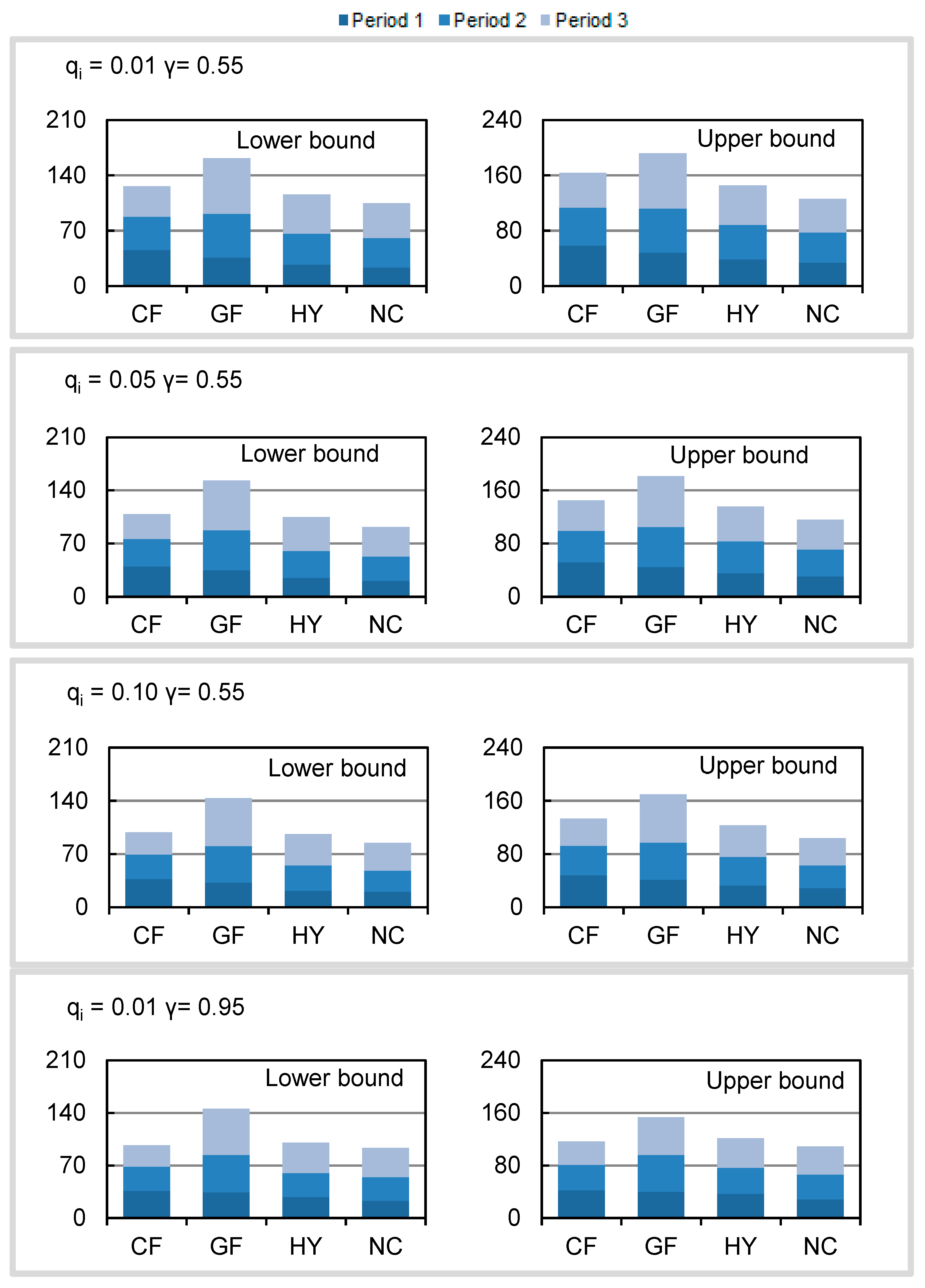
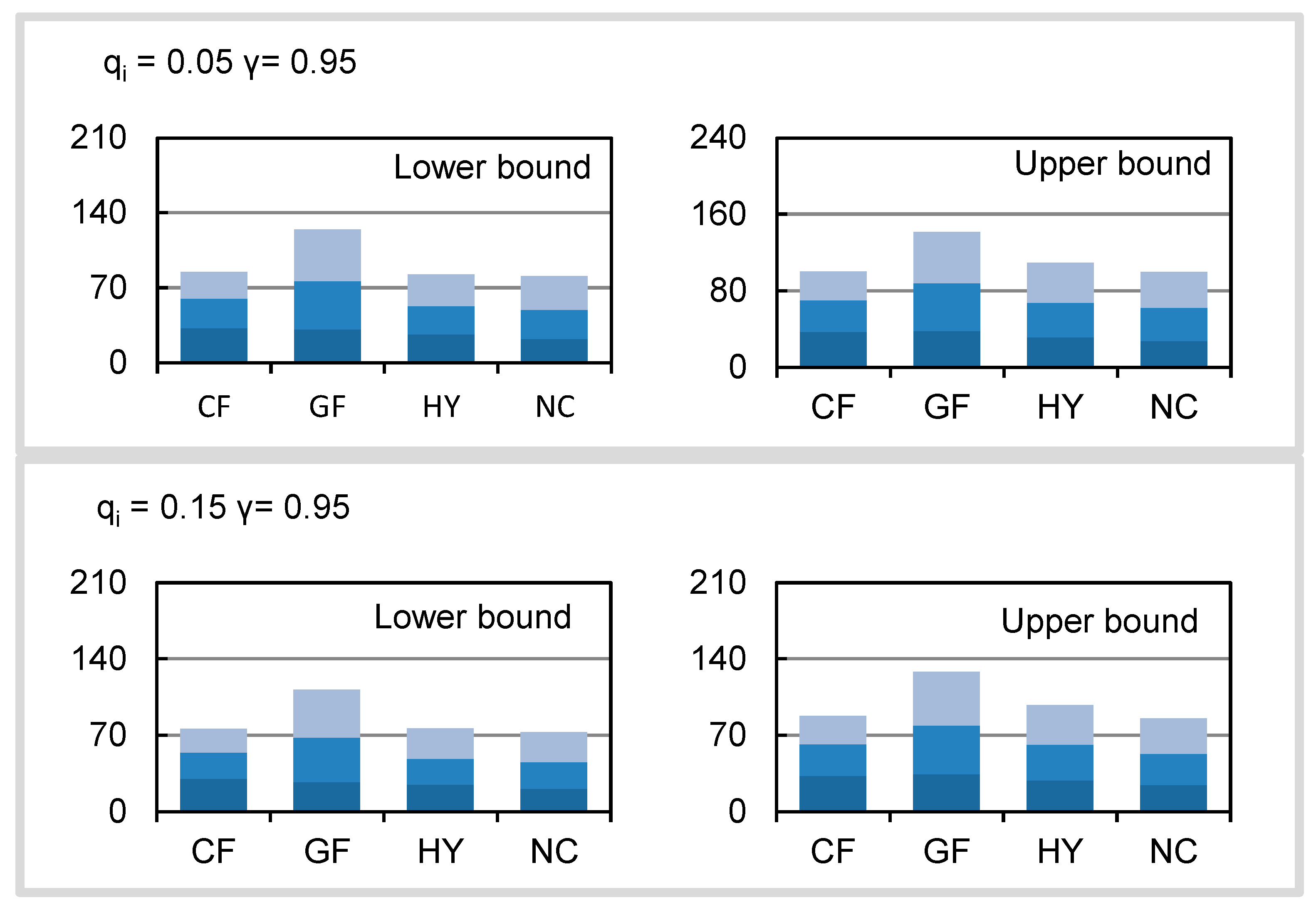
Figure 5 depicts water allocation patterns for electricity generation under different ( = 0.01, 0.05, 0.10) and γ levels (γ = 0.55, 0.99). Symbols “CF”, “GF”, “HY”, and “NC” mean “Coal-fired”, “Gas-fired”, “Hydro”, and “Nuclear” electric power utilities, respectively. It is shown that water allocated to coal-fired power would decrease with time, while other electric power utilities would vary with time. For example, under = 0.01 and γ = 0.55, the amount of water allocated to coal-fired power would be [45.89, 58.71] × 103 m3 in period 1 and [42.21, 54.70] × 103 m3 in period 2. The amount of water allocated to gas-fired power would be [36.41, 48.02] × 103 m3 in period 1 and [55.33, 64.23] × 103 m3 in period 2. Moreover, in periods 2 and 3, gas-fired power would be the main water consumption utility (approximately occupying [31.65, 33.49]% and [33.92, 34.72]% of the total water supply, respectively). Such a change would be attributed to the increased electricity generation, purpose of pollution control (less electricity generated by coal-fired power), and high water consumption rate (gas-fired, hydro, and nuclear electric power utilities). On the other hand, the results show that the water allocation would be as follows: surface water > groundwater > recycled water. Figure 6 summarizes the distribution of water allocation in each period. In period 1, surface water and groundwater would respectively occupy [49.18, 52.77]% and [32.35, 37.98]% of the total water supply, while recycled water would contribute [12.84, 14.88]%. Since the surface water and groundwater allocations are constrained by resource shortage and cost pressure, their share would keep decreasing with time (resulting in a drop of around [5.74, 11.81]% and [3.48, 5.19]% in period 3 compared to period 1). On the contrary, the share of recycled water would keep increasing with time based on the aim of resources conservation.
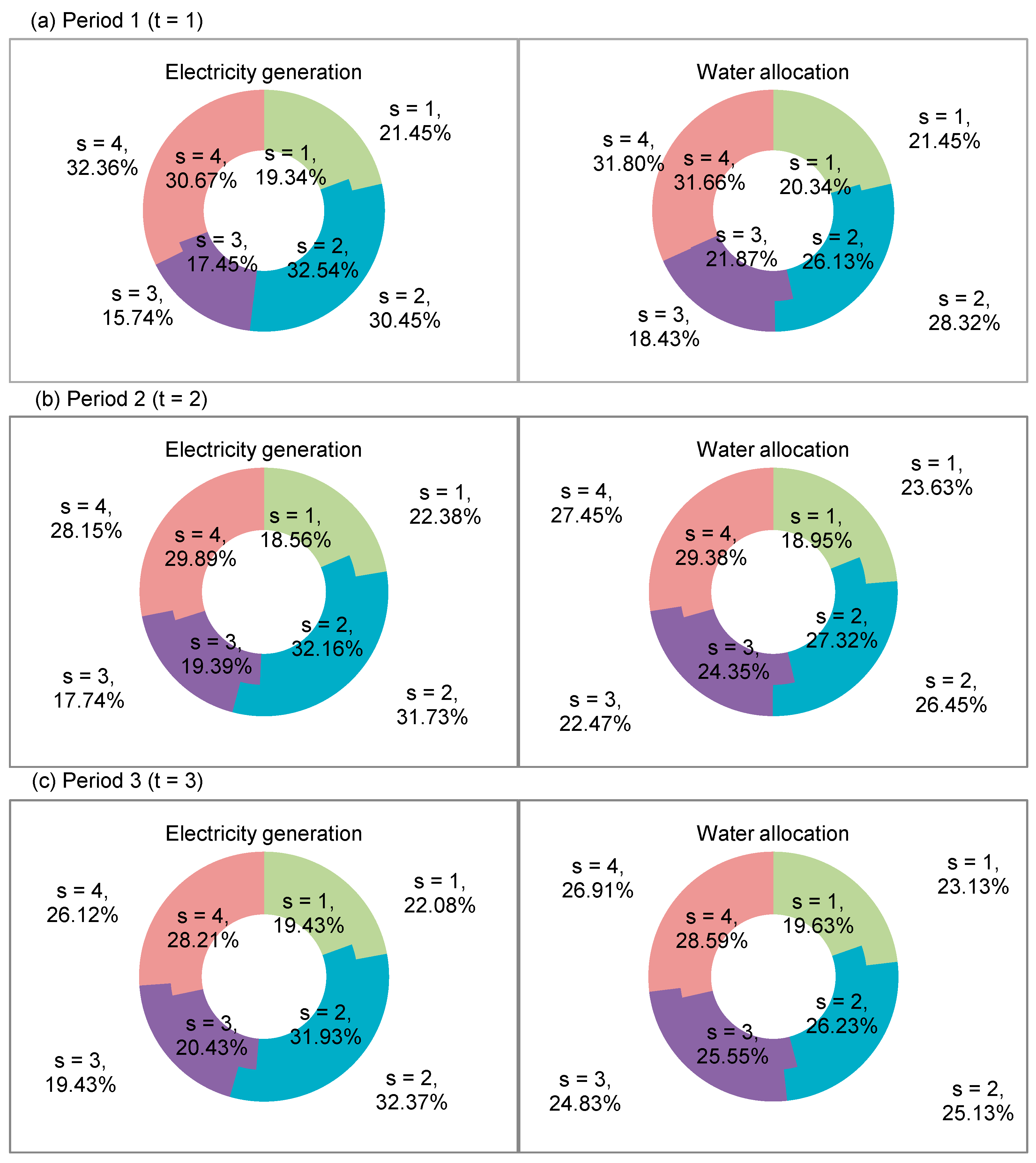
Figure 7 shows the proportion of electricity generation (including gas-fired, coal-fired, hydro, and nuclear power) and water supply in each season. It is indicated that different seasons would correspond to varied electricity generation and water supply patterns. For example, in period 1, the electricity generation and water supply would contribute [19.34, 21.45]% and [20.34, 21.45]% in spring (s = 1), while they would respectively account for [33.54, 31.45]% and [25.13, 28.32]% of the total electricity generation and water allocation in summer (s = 2). Generally, the electricity demand in summer and winter would be higher than that in spring and autumn due to air-conditioning operations (in summer) and heating (in winter). Thus, the share of water supply in winter would reach the highest, while the ratio of water allocation in summer would be less than that in winter due to the contribution of solar power.
4.5. Pollutant Emissions
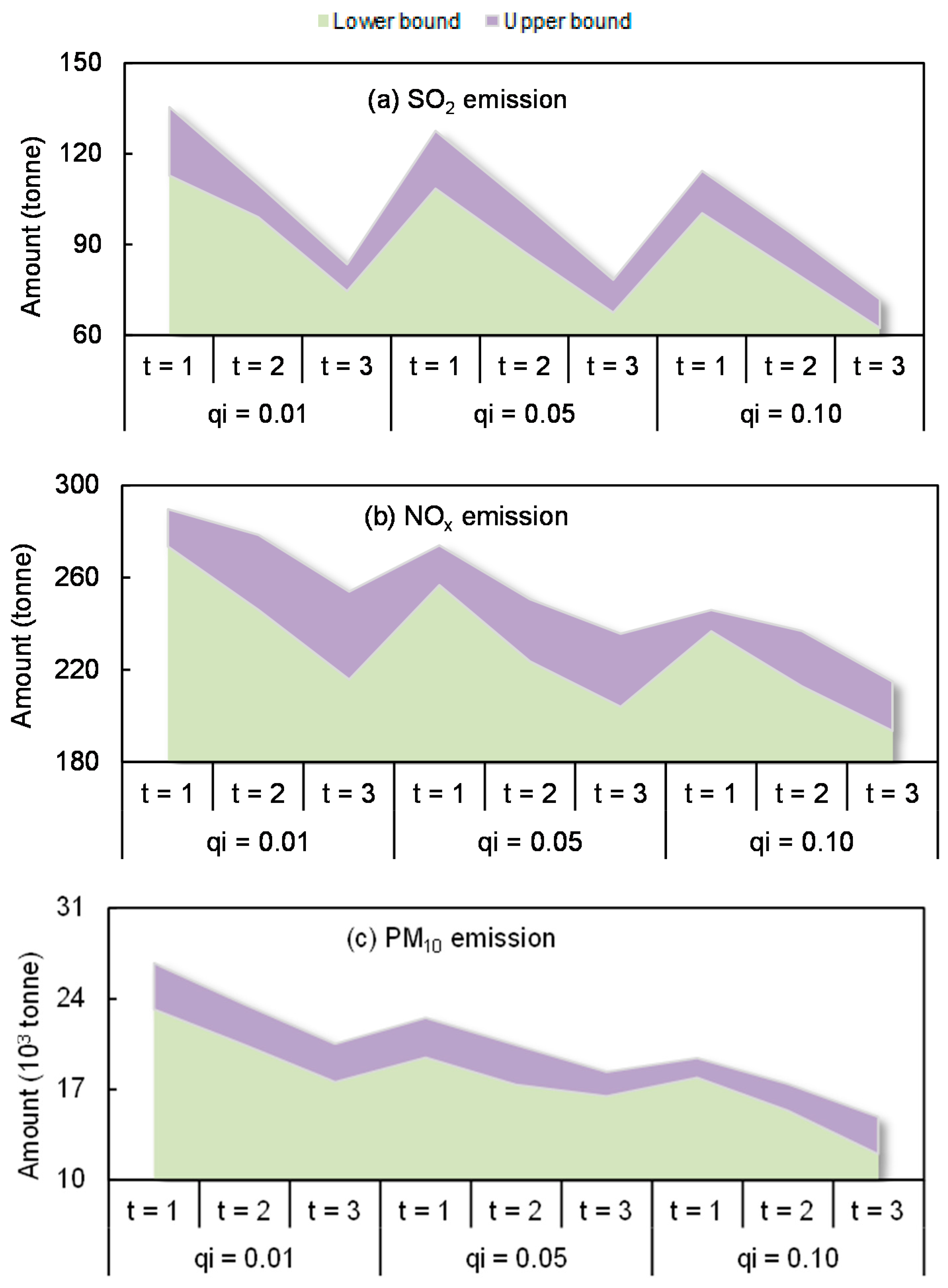
In this study, SO2, NOx, and PM10 are selected as the air pollutants that decision makers want to mitigate due to their harmful impacts on human health and the atmospheric environment. Figure 8 displays the pollutant emissions under each qi level. Results indicate a downtrend of pollutant emissions from period 1 to period 3. Under qi = 0.01, the pollutant emissions (SO2, NOx, and PM10) would decrease by [23.51, 26.34]%, [17.71, 21.34]%, and [23.23, 24.69]% from period 1 to period 3. The downtrend would mainly be associated with the strict emission regulations and enhanced pollutant treatment technology. More technologies which can not only satisfy seasonal peak-electricity demand but also be helpful to promote sustainable development should be selected, such as biomass power generation (e.g., waste incineration, biogas power generation, and landfill gas power generation).
5. Conclusions
In this study, an interval fuzzy-stochastic chance-constrained programming (IFSCP) method was developed by integrating the chance-constrained programming (CCP) method into an interval fuzzy credibility-constrained programming (IFCP) framework. The IFSCP method can tackle multiple uncertainties expressed as possibility distributions, probability distributions, and interval values. Generally speaking, IFCP can deal with possibility distributions and interval values when this type of uncertainty exists in objective and constraints, while CCP has advantages in handling probability distributions. Moreover, whether a particular facility development or expansion option needs to be undertaken, is indicated by the use of integer variables. As a new optimization method, IFSCP integrated the advantages of the above methods, without inheriting the disadvantages of these methods. Then, it can be applied to electric power system (EPS) planning where the energy-water nexus is taken into account, leading to an interval fuzzy-stochastic chance-constrained programming based energy-water nexus (IFSCP-WEN) model. Different credibility (i.e., γ) levels and probability (i.e., ) levels are set to reflect the tradeoffs between water and electricity generation as well as system cost and the constraint-violation risk. Results reveal that: (i) system costs would increase with raised γ levels and decrease with raised levels; (ii) electricity and water supplies would decrease with raised γ and levels due to the changed risk attitudes of decision makers (from risk-neutral attitude to risk-averse attitude) and decreased electricity demand; (iii) imported electricity would vary with the changed electricity generation since the system’s electricity generation cannot satisfy its electricity demand.
In terms of the energy-water nexus, results disclose that the energy supply structure would tend to the transition from coal-dominated into clean energy-dominated (especially natural gas). The ratio of clean energy related power to total electricity generation would respectively be [45.68, 52.87]%, [60.96, 62.68]%, and [71.53, 73.66]% from period 1 to period 3. Correspondingly, water allocated to coal-fired power would decrease with time, while other electric power utilities would vary with time. There would be a drop of approximately [11.37, 17.53]% of water allocation to coal-fired power from period 1 to period 3. Surface water would be the main water source, accounting for [49.18, 52.77]%, [43.64, 47.81]%, and [40.96, 43.44]% of the total water supply. The ratio of recycled water to total water supply would increase by about [11.37, 14.85]%. Besides, the share of water supply in winter would reach the highest level (due to the high electricity demand for heating), while the ratio of water supply in summer (high electricity demand for operating air-conditions) would be less than that in winter due to the contribution of solar power. The pollutant emissions (SO2, NOx, and PM10) would decrease with time due to the strict emission regulations and enhanced pollutant treatment technology.
The first attempt to employ the IFSCP-WEN model to support EPS planning under multiple uncertainties demonstrates its applicability. However, the IFSCP method still has space for further improvement. Actually, with many EPS planning problems, the electricity which is produced by coal combustion can emit large amounts of greenhouse gas (GHG). In such a context, it is also desired to incorporate the energy-GHG nexus into EPS planning, leading to energy-water-GHG based EPS. Moreover, the probability distributions are determined based on the decision makers’ subjective estimation (according to the historical data) and the sensitivity of the solution may be questioned. Support vector regression (SVR) and Monte Carlo simulation can be used to deal with such a concern. On the other hand, a hypothetical but representative study system has been developed for illustrating the applicability of the proposed model based on representative costs and technical data from EPS literature. However, in real-world problems, the extension of power capacity is done together with the transmission and distribution (T&D) lines and the capacity expansion should be analyzed. Meanwhile, the planning horizon is typically 10 or even more years.
Acknowledgments
This research was supported by the State Grid Science & Technology Project (5217L017000N), Beijing Natural Science Foundation (L160011), National Key R&D Program of China (2016YFC0502800), and the Interdiscipline Research Funds of Beijing Normal University. The authors are grateful to the editors and the anonymous reviewers for their insightful comments and suggestions.
Author Contributions
Yongping Li and Guohe Huang conceived and designed the experiments; Yongping Li performed the experiments; Cai Suo and Shuo Yin analyzed the data; Guohe Huang contributed reagents/materials/analysis tools; Jing Liu wrote the paper.
Conflicts of Interest
The authors declare no conflict of interest.
Appendix A. Solution Method
Submodel (1) for (i.e., lower bound of objective function) can be first formulated when the system objective is to be minimized, while submodel (2) corresponding to (i.e., upper bound of objective function) can then be formulated based on the solution of submodel (1):
Submodel (1):
subject to:
Submodel (2):
subject to:
where decision variables with positive coefficients in the objective function, and with negative coefficients. By solving the two submodels, interval solutions with probability and possibility information can be obtained and be used for generating a range of decision options.
Appendix B. Nomenclatures for Parameters and Variables
| system cost over the planning horizon ($) | |
| N | type of generating facility; n = 1 (coal-fired); n = 2 (natural gas-fired); n =3 (hydro); n = 4 (nuclear); n = 5 (solar); n = 6 (wind) |
| T | time period; t = 1, 2, 3 |
| S | season; s = 1 (spring); s = 2 (summer); s = 3 (autumn); s = 4 (winter) |
| unit cost for purchasing energy resource n in period t ($/TJ) | |
| amount of electricity generation via utility n in season s of period t (GWh) | |
| consumption rate of utility n (TJ/GWh) | |
| cost for importing electricity in season s of period t ($/GWh) | |
| imported electricity in season s of period t (GWh) | |
| fixed cost for electricity generation by utility n in period t ($/GW) | |
| expanded capacity for utility n in period t (GW) | |
| 0–1 variables for identifying whether or not utility n needs to be expanded in period t | |
| variable cost for generating electricity via utility n in period t ($/GWh) | |
| service time of utility n in season s of period t (h) | |
| fixed cost for expanding capacity for utility n in period t ($) | |
| variable cost for expanding capacity for utility n in period t ($/GW) | |
| environmental facilities cost for SO2 emission in period t ($/GW) | |
| cost for emission of SO2 in period t ($/GWh) | |
| environmental facilities cost for NOx emission in period t ($/GW) | |
| cost for emission of NOx in period t ($/GWh) | |
| environmental facilities cost for PM10 emission in period t ($/GW) | |
| cost for emission of PM10 in period t ($/GWh) | |
| financial subsidy in period t ($/GWh) | |
| available resource for utility n in period t (TJ) | |
| unit cost of groundwater for electricity generation ($/m3) | |
| groundwater for electricity generation by utility n in season s of period t (m3) | |
| available groundwater in season s of period t (m3) | |
| unit cost of surface water for electricity generation ($/m3) | |
| surface water for electricity generation by utility n in season s of period t (m3) | |
| available surface water in season s of period t (m3) | |
| unit cost of recycled water for electricity generation ($/m3) | |
| recycled water for electricity generation by utility n in season s of period t (m3) | |
| available recycled water in season s of period t (m3) | |
| residual capacity for utility n (GW) | |
| base-load electricity demand in period t (GWh) | |
| peak-electricity demand in season s of period t (GWh) | |
| unit amount of electricity for pumping groundwater in season s of period t (GWh/m3) | |
| unit amount of electricity for extracting surface water in season s of period t (GWh/m3) | |
| unit amount of electricity for delivering water in season s of period t (GWh/m3) | |
| available electricity for extracting and delivering water in season s of period t (GWh) | |
| unit amount of electricity for treating wastewater in season s of period t (GWh/m3) | |
| unit amount of electricity for recycling water in season s of period t (GWh/m3) | |
| available electricity for recycled water in season s of period t (GWh) | |
| consumption rate of electricity for collecting, treating and delivering water (%) | |
| unit water demand per unit of electricity generation (m3/GWh) | |
| emission amount of SO2 in utility n in period t (tonne/GWh) | |
| emission amount of NOX in utility n in period t (tonne/GWh) | |
| emission amount of PM10 in facility n in period t (tonne/GWh) | |
| allowed amount of SO2 in period t (tonne) | |
| allowed amount of NOX in period t (tonne) | |
| allowed amount of PM10 in period t (tonne) | |
| maximum capacity for electricity generation facility n (GW) |
References
- World Energy Outlook Report; International Energy Agency: Paris, France, 2010. Available online: http://www.worldenergyoutlook.org (accessed on 14 November 2017).
- Yoon, S.G.; Kang, S.G. Economic microgrid planning algorithm with electric vehicle charging demands. Energies 2017, 10, 1487. [Google Scholar] [CrossRef]
- Nair, S.; George, B.; Malano, H.M.; Arora, M.; Nawarathna, B. Water-energy-greenhouse gas nexus of urban water systems: Review of concepts, state-of-art and methods. Resour. Conserv. Recycl. 2014, 89, 1–10. [Google Scholar] [CrossRef]
- Ozturk, I. Sustainability in the food-energy-water nexus: Evidence from BRICS (Brazil, the Russian Federation, India, China, and South Africa) countries. Energy 2015, 93, 999–1010. [Google Scholar] [CrossRef]
- DeNooyer, T.A.; Peschel, J.M.; Zhang, Z.X.; Stillwell, A.S. Integrating water resources and power generation: The energy-water nexus in Illinois. Appl. Energy 2016, 162, 363–371. [Google Scholar] [CrossRef]
- Vilanova, M.R.N.; Balestier, J.A.P. Exploring the energy-water nexus in Brazil: The electricity use for water supply. Energy 2015, 85, 415–432. [Google Scholar] [CrossRef]
- Gleick, P.H. Water and Energy. Annu. Rev. Energy Environ. 1994, 19, 267–299. [Google Scholar] [CrossRef]
- Yang, J.; Chen, B. Energy-water nexus of wind power generation systems. Appl. Energy 2016, 169, 1–13. [Google Scholar] [CrossRef]
- Davies, E.G.R.; Kyle, P.; Edmonds, J.A. An integrated assessment of global and regional water demands for electricity generation to 2095. Adv. Water Resour. 2013, 52, 296–313. [Google Scholar] [CrossRef]
- Santhosh, A.; Farid, A.M.; Youcef-Toumi, K. Real-time economic dispatch for the supply side of the energy-water nexus. Appl. Energy 2014, 122, 42–52. [Google Scholar] [CrossRef]
- Li, P.; Chen, B.; Li, Z.L.; Jing, L. ASOC: A novel agent-based simulation-optimization coupling approach-algorithm and application in offshore oil spill responses. J. Environ. Inform. 2016, 28, 90–100. [Google Scholar]
- Khan, Z.; Linares, P.; García-González, J. Integrating water and energy models for policy driven applications. A review of contemporary work and recommendations for future developments. Renew. Sustain. Energy Rev. 2017, 67, 1123–1138. [Google Scholar] [CrossRef]
- Bazilian, M.; Rogner, H.; Howells, M.; Hermann, S.; Arent, D.; Gielen, D.; Pasquale, S.; Alexander, M.; Paul, K.; Richard, S.J.T.; et al. Considering the energy, water and food nexus: Towards an integrated modelling approach. Energy Policy 2011, 39, 7896–7906. [Google Scholar] [CrossRef]
- Dubreuil, A.; Assoumou, E.; Bouckaert, S.; Selosse, S.; Maizi, N. Water modeling in an energy optimization framework—The water-scarce middle east context. Appl. Energy 2013, 101, 268–279. [Google Scholar] [CrossRef]
- Vliet Van, M.T.H.; Vögele, S.; Rübbelke, D. Water constraints on European power supply under climate change: Impacts on electricity prices. Environ. Res. Lett. 2013, 8, 1345–1346. [Google Scholar] [CrossRef]
- Liu, L.; Hejazi, M.; Patel, P.; Kyle, P.; Davies, E.; Zhou, Y.Y.; Clarke, L.; Edmonds, J. Water demands for electricity generation in the U.S.: Modeling different scenarios for the energy-water nexus. Technol. Forecast. Soc. Chang. 2015, 94, 318–334. [Google Scholar] [CrossRef]
- Lubega, W.N.; Farid, A.M. Quantitative engineering systems modeling and analysis of the energy-water nexus. Appl. Energy 2014, 135, 142–157. [Google Scholar] [CrossRef]
- Santhosh, A.; Farida, A.M.; Youcef-Toumic, K. The impact of storage facility capacity and ramping capabilities on the supply side economic dispatch of the energy-water nexus. Energy 2014, 66, 363–377. [Google Scholar] [CrossRef]
- Gjorgiev, B.; Sansavini, G.; Gjorgiev, B.; Sansavini, G.; Gjorgiev, B.; Sansavini, G. Electrical power generation under policy constrained energy-water nexus. Appl. Energy 2017. [Google Scholar] [CrossRef]
- Nie, S.; Li, Y.P.; Liu, J.; Huang, C.Z. Risk management of energy system for identifying optimal power mix with financial-cost minimization and environmental-impact mitigation under uncertainty. Energy Econ. 2017, 61, 313–329. [Google Scholar] [CrossRef]
- Li, Y.P.; Huang, G.H.; Yang, Z.F.; Nie, S.L. IFMP: Interval-fuzzy multistage programming for water resources management under uncertainty. Resour. Conserv. Recycl. 2008, 52, 800–812. [Google Scholar] [CrossRef]
- Zhang, Y.; Huang, G. Optimal water resource planning under fixed budget by interval-parameter credibility constrained programming. Eng. Optim. 2011, 43, 879–889. [Google Scholar] [CrossRef]
- Marufuzzaman, M.; Eksioglua, S.D.; Huang, E. Two-stage stochastic programming supply chain model for biodiesel production via wastewater treatment. Comput. Oper. Res. 2014, 49, 1–17. [Google Scholar] [CrossRef]
- Seddighi, A.H.; Ahmadi-Javid, A. Integrated multiperiod power generation and transmission expansion planning with sustainability aspects in a stochastic environment. Energy 2015, 86, 9–18. [Google Scholar] [CrossRef]
- Ghalelou, A.N.; Fakhri, A.P.; Nojavan, S.; Majidi, M.; Hatami, H. A stochastic self-scheduling program for compressed air energy storage (CAES) of renewable energy sources (RESs) based on a demand response mechanism. Energy Convers. Manag. 2016, 120, 388–396. [Google Scholar] [CrossRef]
- Taylan, O.; Kaya, D.; Demirbas, A. An integrated multi attribute decision model for energy efficiency processes in petrochemical industry applying fuzzy set theory. Energy Convers. Manag. 2016, 117, 501–512. [Google Scholar] [CrossRef]
- Theo, W.L.; Lim, J.S.; Alwi, S.R.W.; Rozali, N.E.M.; Ho, W.S.; Abdul-Manan, Z. An MILP model for cost-optimal planning of an on-grid hybrid power system for an eco-industrial park. Energy 2016, 116, 1423–1441. [Google Scholar] [CrossRef]
- Wu, Y.N.; Xie, C.; Xu, C.; Li, F. A decision framework for electric vehicle charging station site selection for residential communities under an intuitionistic fuzzy environment: A case of Beijing. Energies 2017, 10, 1270. [Google Scholar] [CrossRef]
- Tan, Q.L.; Ding, Y.H.; Zhang, Y.M. Optimization model of an efficient collaborative power dispatching system for carbon emissions trading in China. Energies 2017, 10, 1405. [Google Scholar] [CrossRef]
- Soares, M.P.; Street, A.; Valladão, D.M. On the solution variability reduction of stochastic dual dynamic programming applied to energy planning. Eur. J. Oper. Res. 2017, 258, 743–760. [Google Scholar] [CrossRef]
- Dai, C.; Cai, Y.P.; Ren, W.; Xie, Y.F.; Guo, H.C. Identification of optimal placements of best management practices through an interval-fuzzy possibilistic programming model. Agric. Water Manag. 2016, 165, 108–121. [Google Scholar] [CrossRef]
- Li, Y.P.; Huang, G.H.; Huang, Y.F.; Zhou, Y.F. A multistage fuzzy-stochastic programming model for supporting sustainable water resources allocation and management. Environ. Model. Softw. 2009, 24, 786–797. [Google Scholar] [CrossRef]
- Li, Y.F.; Li, Y.P.; Huang, G.H.; Chen, X. Energy and environmental systems planning under uncertainty—An inexact fuzzy-stochastic programming approach. App. Energy 2010, 87, 3189–3211. [Google Scholar] [CrossRef]
- Li, Y.P.; Huang, G.H. Electric-power systems planning and greenhouse-gas emission management under uncertainty. Energy Convers. Manag. 2012, 57, 173–182. [Google Scholar] [CrossRef]
- Liu, J.; Li, Y.P.; Huang, G.H. Mathematical modeling for water quality management under interval and fuzzy uncertainties. J. Appl. Math. 2013, 2013, 731568. [Google Scholar] [CrossRef]
- Khan, U.T.; Valeo, C. Short-term peak flow rate prediction and flood risk assessment using fuzzy linear regression. J. Environ. Inform. 2016, 28, 71–89. [Google Scholar]
- Yu, L.; Li, Y.P.; Huang, G.H. A fuzzy-stochastic simulation-optimization model for planning electric power systems with considering peak-electricity demand: A case study of Qingdao, China. Energy 2016, 98, 190–203. [Google Scholar] [CrossRef]
- Hamiche, A.M.; Stambouli, A.B.; Flazi, S. A review of the energy-water nexus. Renew. Sustain. Energy Rev. 2016, 65, 319–331. [Google Scholar] [CrossRef]
- Li, Y.P.; Huang, G.H.; Nie, S.L. Planning water resources management system using a fuzzy-boundary interval-stochastic programming method. Adv. Water Resour. 2010, 33, 1105–1117. [Google Scholar] [CrossRef]
- Hyndman, R.J.; Fan, S. Density forecasting for long-term peak electricity demand. IEEE Trans. Power Syst. 2010, 25, 1142–1153. [Google Scholar] [CrossRef]
- Statistics Bureau of Qingdao Municipality. Qingdao Statistical Yearbook in 2014; China Statistical Press: Qingdao, China, 2015. (In Chinese) [Google Scholar]
Figure 1.
Framework of the IFSCP-WEN model.

Figure 2.
System cost under each level and γ level. (a) = 0.01; (b) = 0.05; (c) = 0.10.


Figure 3.
Electricity and water supply patterns under each level and γ level: (a) imported electricity; (b) electricity generation; (c) water supply.
Figure 3.
Electricity and water supply patterns under each level and γ level: (a) imported electricity; (b) electricity generation; (c) water supply.

Figure 4.
Distribution of electricity generation in each period: (a) period 1 (t = 1); (b) period 2 (t = 2); (c) period 3 (t = 3).
Figure 4.
Distribution of electricity generation in each period: (a) period 1 (t = 1); (b) period 2 (t = 2); (c) period 3 (t = 3).

Figure 5.
Water allocation patterns for electricity generation under different and γ levels. (Note: “CF” denotes “Coal-fired”; “GF” denotes “Gas-fired”; “HY” denotes “Hydro”; “NC” denotes “Nuclear”).
Figure 5.
Water allocation patterns for electricity generation under different and γ levels. (Note: “CF” denotes “Coal-fired”; “GF” denotes “Gas-fired”; “HY” denotes “Hydro”; “NC” denotes “Nuclear”).


Figure 6.
Distribution of water allocation in each period: (a) period 1 (t = 1); (b) period 2 (t = 2); (c) period 3 (t = 3).
Figure 6.
Distribution of water allocation in each period: (a) period 1 (t = 1); (b) period 2 (t = 2); (c) period 3 (t = 3).

Figure 7.
Proportion of electricity generation and water supply in each season: (a) period 1 (t = 1); (b) period 2 (t = 2); (c) period 3 (t = 3).
Figure 7.
Proportion of electricity generation and water supply in each season: (a) period 1 (t = 1); (b) period 2 (t = 2); (c) period 3 (t = 3).

Figure 8.
Pollutant emissions under each level: (a) SO2 emission; (b) NOx emission; (c) PM10 emission.
Figure 8.
Pollutant emissions under each level: (a) SO2 emission; (b) NOx emission; (c) PM10 emission.


Table 1.
Costs for electricity generation.
| Technology | Period | ||
|---|---|---|---|
| t = 1 | t = 2 | t = 3 | |
| Fixed cost for electricity generation (106 $/GW) | |||
| Coal-fired | [(22.45, 23.38, 25.24), (28.06, 30.12, 33.07)] | [(21.24, 22.91, 24.43), (27.17, 28.38, 32.11)] | [(20.98, 22.44, 23.68), (25.83, 26.92, 31.54)] |
| Gas-fired | [(33.16, 35.68, 37.75), (40.32, 42.81, 44.93)] | [(30.23, 33.17, 35.22), (37.44, 39.81,41.75)] | [(29.23, 31.23,33.74), (35.78, 37.47, 39.87)] |
| Hydro | [(71.47, 73.36, 75.13), (86.71, 88.03, 89.94)] | [(67.34, 69.38, 71.03), (81.54, 83.26,85.76)] | [(63.35, 65.43, 67.76), (75.87, 78.51, 80.65)] |
| Nuclear | [(115.33, 119.21, 121.74), (140.27, 143.04, 145.84)] | [(111.74, 113.17, 115.83), (133.23, 135.81, 137.34)] | [(104.34, 107.39, 110.54), (126.43, 128.87, 131.43)] |
| Solar | [(67.43, 70.26, 72.54), (81.74, 84.31, 86.47)] | [(63.54, 66.71, 68.95), (77.98, 80.06, 82.97)] | [(60.76, 63.36, 66.02), (72.43, 75.96, 78.42)] |
| Wind | [(55.54, 59.25, 62.54), (68.43, 71.21, 74.04)] | [(52.54, 56.26, 59.75), (63.03, 67.51, 71.75)] | [(51.17, 53.38, 55.93), (61.42, 64.06, 66.84)] |
| Variable cost for electricity generation (103 $/GWh) | |||
| Coal-fired | [(1.34, 1.59, 1.84), (1.72, 1.91, 2.11)] | [(1.31, 1.56, 1.59), (1.85, 1.88, 1.91)] | [(1.49, 1.52, 1.55), (1.81, 1.84, 1.87)] |
| Gas-fired | [(2.14, 2.19, 2.24), (2.58, 2.63, 2.68)] | [(2.03, 2.08, 2.13), (2.46, 2.51, 2.55)] | [(1.92, 1.97, 2.02), (2.31, 2.36, 2.41)] |
| Hydro | [(7.21, 7.25, 7.29), (8.63, 8.67, 8.71)] | [(6.81, 6.85, 6.89), (8.17, 8.21, 8.25)] | [(6.44, 6.48, 6.52), (7.71, 7.75, 7.79)] |
| Nuclear | [(7.17, 7.21, 7.25), (8.53, 8.57, 8.61)] | [(6.83, 6.87, 6.91), (8.18, 8.22, 8.26)] | [(6.45, 6.49, 6.53), (7.74, 7.79, 7.83)] |
| Solar | [(7.74, 7.79, 7.83), (9.32, 9.36, 9.40)] | [(7.55, 7.59, 7.63), (9.26, 9.30, 9.34)] | [(7.43, 7.47, 7.51), (9.11, 9.15, 9.19)] |
| Wind | [(9.42, 9.47, 9.52), (11.29, 11.34, 11.39)] | [(9.01, 9.06, 9.11), (10.81, 10.86, 10.91)] | [(8.61, 8.66, 8.71), (10.33, 10.38, 10.43)] |
Table 2.
Energy-water nexus related data.
| Technology | Period | ||
|---|---|---|---|
| t = 1 | t = 2 | t = 3 | |
| Unit Water Demand of Electricity Generation (103 m3/GWh) | |||
| Coal-fired | [(1.22, 1.26.1.32), (1.48, 1.53, 1.58)] | [(1.14, 1.21, 1.27), (1.41, 1.46, 1.52)] | [(1.07, 1.14, 1.19), (1.32, 1.37, 143)] |
| Gas-fired | [(1.71, 1.76, 1.82), (2.14, 2.23, 2.29)] | [(1.62, 1.69, 1.74), (2.03, 2.14, 2.22)] | [(1.52, 1.59, 1.65), (1.85, 1.94, 2.03)] |
| Hydro | [(2.78, 2.84, 2.93), (3.21, 3.53, 3.71)] | [(2.21, 2.47, 2.63), (3.13, 3.26, 3.45)] | [(2.24, 2.48, 2.75), (2.85, 2.94, 3.12)] |
| Nuclear | [(1.84, 1.89, 1.93), (2.29, 2.37, 2.45)] | [(1.63, 1.72, 1.79), (2.07, 2.15, 2.21)] | [(1.57, 1.62, 1.68), (1.83, 1.95, 2.03)] |
| Unit Amount of Electricity for Extracting Water (10-6 GWh/m3) | |||
| Surface water | [(0.76, 0.81, 0.86), (0.89, 0.94, 0.99)] | [(0.71, 0.78, 0.83), (0.84, 0.89, 0.94)] | [(0.63, 0.75, 0.79), (0.81, 0.85, 0.89)] |
| Groundwater | [(0.36, 0.42, 0.48), (0.51, 0.57, 0.63)] | [(0.32, 0.38, 0.44), (0.47, 0.53, 0.59)] | [(0.27, 0.33, 0.39), (0.42, 0.48, 0.54)] |
| Unit Amount of Electricity for Delivering Water (10-6 GWh/m3) | |||
| Surface water | [(1.21 1.23, 1.25), (1.31, 1.33, 1.35)] | [(1.17, 1.19, 1.21), (1.25, 1.27, 1.29)] | [(1.14, 1.16, 1.18), (1.22, 1.24, 1.26)] |
| Groundwater | [(1.21 1.23, 1.25), (1.31, 1.33, 1.35)] | [(1.17, 1.19, 1.21), (1.25, 1.27, 1.29)] | [(1.14, 1.16, 1.18), (1.22, 1.24, 1.26)] |
| Recycled water | [(0.23, 0.26, 0.29), (0.31, 0.34, 0.37)] | [(0.19, 0.22, 0.25), (0.27, 0.30, 0.33)] | [(0.14, 0.17, 0.20), (0.23, 0.26, 0.29)] |
| Unit Amount of Electricity for Treating Water(10-6 GWh/m3) | |||
| Recycled water | [(0.12, 0.13, 0.14), (0.16, 0.17, 0.18)] | [(0.10, 0.11, 0.12), (0.14, 0.15, 0.16)] | [(0.09, 0.10, 0.11), (0.13, 0.14, 0.15)] |
Table 3.
Electricity demand under different levels.
| Technology | Period | ||
|---|---|---|---|
| t = 1 | t = 2 | t = 3 | |
| Annual Electricity Demand (103 GWh) | |||
| = 0.01 | [69.84, 74.34] | [76.39, 79.03] | [81.42, 85.03] |
| = 0.05 | [65.38,67.43] | [71.34, 75.23] | [76.27, 79.49] |
| = 0.10 | [55.73,63.69] | [65.84, 69.32] | [71.43, 74.43] |
| Electricity Demand in Summer (103 GWh) | |||
| = 0.10 | [28.94, 32.48] | [34.18, 37.49] | [39.43, 42.55] |
| = 0.05 | [24.04, 27.03] | [29.75, 33.07] | [35.94, 38.94] |
| = 0.01 | [19.43, 23.57] | [24.43, 27.03] | [29.74, 34.43] |
| Electricity Demand in Winter (103 GWh) | |||
| = 0.01 | [22.53, 27.84] | [28.39, 31.38] | [35.57, 38.15] |
| = 0.05 | [19.37, 21.33] | [23.03, 26.14 ] | [31.28, 34.47] |
| = 0.10 | [15.46, 18.47] | [20.03, 24.07] | [26.54, 30.74] |
© 2017 by the authors. Licensee MDPI, Basel, Switzerland. This article is an open access article distributed under the terms and conditions of the Creative Commons Attribution (CC BY) license (http://creativecommons.org/licenses/by/4.0/).
Share and Cite
MDPI and ACS Style
Liu, J.; Li, Y.; Huang, G.; Suo, C.; Yin, S. An Interval Fuzzy-Stochastic Chance-Constrained Programming Based Energy-Water Nexus Model for Planning Electric Power Systems. Energies 2017, 10, 1914. https://doi.org/10.3390/en10111914
AMA Style
Liu J, Li Y, Huang G, Suo C, Yin S. An Interval Fuzzy-Stochastic Chance-Constrained Programming Based Energy-Water Nexus Model for Planning Electric Power Systems. Energies. 2017; 10(11):1914. https://doi.org/10.3390/en10111914
Chicago/Turabian StyleLiu, Jing, Yongping Li, Guohe Huang, Cai Suo, and Shuo Yin. 2017. "An Interval Fuzzy-Stochastic Chance-Constrained Programming Based Energy-Water Nexus Model for Planning Electric Power Systems" Energies 10, no. 11: 1914. https://doi.org/10.3390/en10111914
Note that from the first issue of 2016, this journal uses article numbers instead of page numbers. See further details here.