Modeling of Electricity Demand for Azerbaijan: Time-Varying Coefficient Cointegration Approach


1
King Abdullah Petroleum Studies and Research Center, PO Box 88550, Riyadh 11672, Saudi Arabia
2
Department of Statistics, Azerbaijan State University of Economics (UNEC), Istiqlaliyyat Str. 6, Baku AZ1141, Azerbaijan
3
Institute for Scientific Research on Economic Reforms, 88a, Hasan Bey Zardabi Avenue, Baku AZ1011, Azerbaijan
4
Research Program on Forecasting, Economics Department, The George Washington University, 2115 G Street, NW, Washington, DC 20052, USA
5
Institute of Control Systems, Azerbaijan National Academy of Sciences, B. Vahabzade Street 9, Baku AZ1141, Azerbaijan
6
Department of Economics, University of Perugia, Via Pascoli 20, 06123 Perugia, Italy
7
Department of International Relations, Baku Engineering University, Hasan Aliyev 120, Khirdalan AZ0101, Azerbaijan
*
Author to whom correspondence should be addressed.
Energies 2017, 10(11), 1918; https://doi.org/10.3390/en10111918
Submission received: 31 October 2017
/
Revised: 15 November 2017
/
Accepted: 17 November 2017
/
Published: 21 November 2017
Abstract
:Recent literature has shown that electricity demand elasticities may not be constant over time and this has investigated using time-varying estimation methods. As accurate modeling of electricity demand is very important in Azerbaijan, which is a transitional country facing significant change in its economic outlook, we analyze whether the response of electricity demand to income and price is varying over time in this economy. We employed the Time-Varying Coefficient cointegration approach, a cutting-edge time-varying estimation method. We find evidence that income elasticity demonstrates sizeable variation for the period of investigation ranging from 0.48% to 0.56%. The study has some useful policy implications related to the income and price aspects of the electricity consumption in Azerbaijan.
1. Introduction
The response of electricity demand to economic variables has been widely investigated in the literature, with numerous econometric techniques, parametric [1,2] and non-parametric [3] ranging from aggregate national time series [4,5] country panels [6,7] to regional and household micro data [8,9]. Results have shown a variety of empirical quantifications for price and income elasticities, in the short and in the long run (e.g., [1,10,11]).
Note that most of the existing empirical literature on electricity demand shows constant parameter estimation, with few addressing the issue of parameter instability (e.g., [12] use Kalman filter; for a recent survey of other methods see: [13]), despite the findings of a number of theoretical and empirical studies, which indicate that structural breaks in relations and hence estimated parameters lead to inconsistent inferences and thereby wrong policy decisions. For example, as [14] concluded that the assumption of constant elasticities has to be questionable, they ended up that the income and price elasticities may not be constant. Further, the study explains the differences in income elasticities with the factors such as “… the efficiency of new appliances and the efficiency of the stock demands much lower energy per dollar used to purchase energy consuming goods than many years ago” [14].
Chang and Martinez-Chombo [15] put forward the idea that the model with constant elasticities is debatable due to the changes occurring during the long period of time in the overall economy, which affect the demand for electricity. As examples of the determinants for such changes, the study gives specific factors such as the efficiency improvements in electrical equipment, the developmental stage of the economy, and even the government energy policy and the habit persistence of consumers [15]. The study further emphasizes that the factors listed above are not static, and have a tendency to evolve slowly over time and, as a consequence, they persistently change the responses of the aggregated electricity demand to variations in income and prices.
The common conclusion derived from studies such as [16,17,18,19,20] is that fixed coefficient models are unstable to possible structural changes in the economy, consequently making estimates from such models misleading if parameters change with time. Moreover, as [20] discussed, when the policy regimes change individuals change their expectations too, which consequently changes estimated decision rules and under these circumstances the model parameters are unlikely to be stable.
In this context, the aim of this research is to allow for the possibility of varying response of electricity demand to income and price in Azerbaijan. We employ a Time-Varying Coefficient cointegration (TVC) approach, which is the econometric method developed by [21] and detailed and applied by [22] to model electricity demand in Azerbaijan. In our specification, we take price elasticity as a constant, because the price of electricity is centrally regulated and subsidized rather than market driven.
This exercise is especially important in developing and transitional countries, such as Azerbaijan, since they face significant change in their economic outlook [23]. Therefore, modeling and forecasting electricity consumption based on its main drivers can help energy producers to manage their profits, policymakers to take appropriate measures, and government to manage efficiently limited resources for sustainable development.
There are very limited studies investigating electricity demand in Azerbaijan. Hasanov et al. [23] comprehensively reviewed these studies with their advantages and disadvantages. All the earlier studies for Azerbaijan employ conventional econometric methods, where elasticities of electricity consumption with respect to explanatory variables, for example income and price, are assumed to be invariant over time. However, we argue in this paper that one can get suspicious about constancy of the elasticities estimated by the earlier studies. The main reason for this suspect is that the Azerbaijani economy had different and contrasting development stages since its independence in 1991 (see [24] inter alia). Briefly note that the country was in a very deep recession during 1991–1995 with the declining of real GDP per capita by 2.4% per annum, while it witnessed stable socio-economic development in 1996–2003 with the growth rate of real GDP per capita by 8% annually. It faced very rapid economic growth over 2004–2010, and per annum growth rate of the real GDP per capita was 15.4%, which is very huge. The real GDP per capita slowed down in 2011 and 2012 with the growth rates of −1.23% and 0.85%, respectively, and recovered since then. Additionally, Azerbaijan has ranked first in the world in terms of real GDP growth in 2005, 2006 and 2007, being about 26%, 35% and 25%, respectively, according to the World Bank statistics [25].
In 2014, the real GDP growth significantly went down, mainly caused by the oil price drop and related deteriorations in the Azerbaijani economy. The growth rates were 2.0%, 1.1% and −3.1% in 2014, 2015 and 2016, respectively according to the World Bank statistics [25]. Moreover, electricity price was constant at 0.2 manat per kWh over 1990–2006 and then it has been increased by three times and kept constant again as it is administratively adjusted by the government [26]. Thus, in such an environment described above, it is quite reasonable for one to expect that different development regimes can cause changes in the relationship among energy and macroeconomic indicators, which results in inconstancy in estimated income and price elasticities of electricity consumption. Note that this issue has not been addressed in the earlier electricity studies for Azerbaijan.
This study contributes to the existing literature in three ways. The main contribution is that we first use the Time-Varying Coefficient cointegration model to explore electricity demand in Azerbaijan and we find and argue that income elasticity is time varying. There are some key advantages of the TVC method in cointegration framework. For example, in cointegrated regressions, to allow for TVC is much more important compared to the usual stationary regressions. The point is that if you have TVC and ignore it, then you would still expect to have its average value possibly with some bias in a stationary regression. However, this is not true in a cointegrated regression. It is very crucial to model TVC properly in a cointegrated regression. Otherwise, the regression becomes spurious. Put differently, if the true model is a cointegrated regression with TVC but it is estimated using a regression with fixed coefficients, then the regression outcomes would be spurious and totally nonsensical. Second, considering that there are limited studies on electricity consumption in Azerbaijan, we provide additional evidence of the consumption pattern of this country. Third, as Azerbaijan is an example of a resource-rich developing country in transition, we provide a benchmark of analysis, which can be useful for similar countries, which are going through different economic stages.
We found that income elasticity of electricity demand in Azerbaijan demonstrates sizeable variation for the period of investigation ranging from 0.48 to 0.56, which can be seen as an evidence supporting the objective of the current study. The price elasticity is found to be economically significant with an appropriate sign and size, while it is statistically insignificant.
The findings of the study have some policy implications. Policy decisions based on the forecasts or analyses using invariant elasticity should be revised as we found that income elasticity is not constant over time. Moreover, the decision makers in Azerbaijan should expect more electricity demand by economic agents if income level will rise in the short to medium run. Furthermore, the future regulation in electricity tariff would not have a significant impact on the electricity consumption as we believe the findings showed that price elasticity of the electricity consumption is inelastic and insignificant.
The findings and derived policy implications of the study might be useful in similar countries like Azerbaijan.
The paper is organized as follows. The next section reviews the related literature on Azerbaijan electricity, while Section 3 describes the data used. The utilized econometric methodology and employed functional specification are discussed in Section 4. Section 5 covers empirical estimations and discussion. Finally, Section 6 concludes the research.
2. Literature Review
In this section, we review two kinds of studies analyzing electricity consumption: (a) the studies devoted to Azerbaijan since the country is the focus of our paper here; (b) the studies employing TVC approach.
2.1. Previous Studies Investigating Electricity Demand in Azerbaijan
It is noteworthy that as [23] states, there are very limited studies investigating electricity demand in Azerbaijan. We review them below.
Hasanov et al. [23] modeled and forecasted total final electricity consumption in Azerbaijan over the period 1995–2013, employing the demand-side modeling as a theoretical framework. They used different cointegration and error correction methods, namely Johansen, Auto-Regressive Distributed Lags Bounds Testing (ARDLBT), Engle–Granger (EG) with Fully Modified Ordinary Least Squares (FMOLS), Dynamic Ordinary Least Squares (DOLS) and Canonical Cointegration Regression (CCR). They reported that estimated long-run price and income elasticities changes from −0.8 to −1.0 and 0.1 to 0.2, respectively. While estimated short-run price and income elasticities vary from −0.3 to −0.4 and from 0.4 to 0.7, respectively. Furthermore, the study found speed of adjustment coefficients being around negative unity.
Hasanov and Mikayilov [27] explored the residential electricity consumption in Azerbaijan for the period 2000–2012. They used STIRPAT framework and thereby, examined the effects of population age groups and income. STIRPAT is for Stochastic Impacts by Regression on Population, Affluence, and Technology. Please refer to [28,29] for a detailed information. Results from the ARDLBT method showed that income has a negative association with the electricity. Precisely saying, the electricity elasticities with respect to income were −1.33, −1.98 and −0.76 when the age groups of 0–14, 15–64 and 65–above are considered in the estimations, respectively. Finally, they found overcorrection implying that it takes less than a year to adjust if there is disequilibrium in the long-run relationship of the residential electricity consumption.
Bildirici and Kayikci [30] explored economic growth and electricity consumption nexus in the Commonwealth of Independent States, where Azerbaijan is a member. They applied Pedroni co-integration tests and Panel Fully Modified Ordinary Least Squares (FMOLS) and Auto-Regressive Distributed Lag (ARDL) methods to the panel data over the period 1990–2009. The Granger causality test showed that causality runs from GDP to electricity consumption in the short run. However, the nature of causality is bidirectional in the long run. They estimate the income elasticities of the electricity consumption to be 0.52 and 0.77 from the FMOLS and ARDL methods, respectively. They also found that speed of adjustment coefficient is −0.41. The study suffered from some shortcomings. First, the study only considered income (GDP) as a driver of the electricity consumption but other determinants such as price, demographic indicators, and temperature were missed. Second, the study does not analyze the significant changes in electricity system since it ends in 2009. Moreover, like any other panel studies, it cannot capture specific features of the Azerbaijani electricity system.
Klytchnikova [31] analyzed welfare effect of reforms on the Azerbaijani electricity sector. She used data obtained from the Azerbaijan Household Energy Survey, which was conducted by the World Bank over the period 2003 December–2004 January. She concluded that the average price elasticity of electricity demand with respect to electricity price is −0.69. The main shortcoming of the study is that it does not include income measure in the empirical analysis and, therefore, electricity consumption is just a function of its price. This can lead to biased estimation results due to the omission variable bias issue and therefore mislead policy makers. In addition, the study is based on the very short data. Moreover, it ends in the beginning of 2004 and hence does not reflect the recent changes in the Azerbaijan electricity system.
Note that both negative and positive effects of the income elasticity are found in the previous studies. It might be considered as evidence that that income elasticity is not stable and varies over time.
There are also some papers that only forecasted electricity demand in Azerbaijan: [32,33,34,35,36]. We do not review these papers here because (a) they did not investigate impacts of the main drivers, such as price and income on the electricity consumption and, therefore, did not show numerical relationships. Moreover, all of them used only GDP but not any other explanatory variables to generate forecasted values of the electricity; (b) also, they did not report the models/methods that they employed to generate forecasts of the electricity consumption. Thus, the projected values were more likely biased, since other main determinants such as price, population, temperature and others were not taken into consideration.
2.2. Previous Studies Using Time-Varying Methods
As mentioned in the Introduction section, one of our constitutions in this study is about applying TVC, a recently developed econometric method. In this regard, we review some studies below, where TVC method is applied.
Chang et al. [22] modeled Korean residential, commercial and industrial electricity consumptions using demand-side modeling framework, where income/output, price and temperature were the drivers. This is the seminal study that leads to an extensive using of TVC approach by many other works. They discussed the TVC approach that is developed by [21] in detail. They found that income elasticity varies over time, reflecting rapid development of the Korean economy.
Chang and Chang and Martinez-Chombo [15] examined electricity consumption of Mexican residential, commercial and industrial sectors using demand-side modeling framework. They applied TVC method to the data over the 1985M01–2005M05 and found that income elasticity increases while price elasticity is statistically insignificant over the analyzed period.
Arisoy and Ozturk [12] investigated income and price effects of industrial and residential electricity consumption in Turkey over the period 1960–2008. In order to account for time-varying features of the income and price elasticities, the study employed the Kalman filter approach. They found that the price and income elasticity of residential and industrial electricity demand are generally stable over time.
Inglesi-Lotz [37], who also used the Kalman filter method, examined the impacts of GDP and electricity price on aggregate electricity consumption in South Africa over the period 1980–2005. The study found decreasing price elasticity and increasing income elasticity over the considered period.
Adom [38] investigated the impact of real per capita income, industry electricity intensity, and economic structure on aggregate electricity consumption in Ghana over the period 1971–2008 within the demand-side modeling framework. The study employed rolling regression to reveal how elasticities vary over time. The results from the regression showed that electricity consumption elasticities with respect to the mentioned explanatory variables vary over time. These variations mainly happened in the periods in which policy regime changes. Although the study used demand-side modeling framework as mentioned above, it did not include price, one of the key determinants of the framework, in the analysis. Additionally, the study did not test for cointegration among the variables before estimating their level relationship.
Chang and Hsing [39] tested appropriateness of conventional double-logarithm and linear form methods in analyzing electricity demand in the U.S. over the period 1950–1987. They rejected relevancy of the methods and, hence, adopted a special specification, in which time-varying features of the coefficients could be accounted. The study found that electricity consumption elasticities with respect to own-price, natural gas price and income vary, precisely speaking, was declining over the period. One of the concerns on the reliability of the results derived from the study was that either unit root test or cointegration test was not performed. As discussed in [40] among others, if there is no cointegration among variables in interest, then the level regression is spurious. In addition, the specification that the authors adopted was only able to test double logarithm and linear specifications.
3. Data
In line with the employed model specification, the utilized data is described below. All data are annual for the period from 1990 to 2014. The period is considered based on the data availability. We were not able to take data for earlier years than 1990 because Azerbaijan got its independence in this year. Regarding the end date of our estimation period, electricity consumption data for Azerbaijan sourced from the IEA was only available up to 2014 at the time of conducting this research.
E is per capita electricity consumption, which is equal to total final electricity consumption in TWh divided by population in millions. The total final electricity consumption data are collected from the International Energy Agency Database (IEA) in Mtoe and then converted to TWh in order to be consistent with the electricity price [41]. Population data are taken from the World Bank Database [25].
P is the real electricity price. Nominal retail electricity prices (in Azerbaijani Manat (AZN)) are centrally administrated by the government (being the same for the industrial, residential, and commercial sectors). These data are collected from the various Statistical Yearbooks of the State Statistical Committee of the Republic of Azerbaijan [42]. The real electricity prices are in 2005 AZN, found by deflating the nominal prices by the Consumer Price Index (CPI), 2005 = 100 collected from [42].
GDP is real total GDP per capita in USD using Purchasing Power Parity. It is taken from the International Energy Agency Database [41].
Note that, in the estimations, the small letters such as e, p and gdp represent the natural logarithmic transformations of the corresponding capital letters. The graphs of the logarithmic transformations of the variables and their growth rates are depicted in Figure 1.
Note that the horizontal axes indicate years while the vertical axes shows the natural logarithm scale.
4. Econometric Methodology
4.1. Unit Root Tests
4.2. Time-Varying Coefficient Cointegration Approach
A typical residential electricity demand function (This Section Adapted from [22]) is a log-linear function with fixed coefficients (FC), which relates demand of electricity and its main drivers such as electricity price, income, etc. ([45] inter alia). In our study, we utilized the specification as did [12]. This model can be written as follows:
for t = 1, ..., T, where yt is electricity demand, xt is income, pt is electricity price (all three in logarithmic form); α is the income elasticity of electricity demand, β is price elasticity of electricity demand, vt is disequilibrium error and τ is constant term.
The idea behind TVC is that building on the benchmark FC model in Equation (1) allows for the possibility of a time-varying long-run elasticity that is a smooth function of time. A constant elasticity is nested as a special case that can be tested empirically. In this sense, the time is used as a proxy for unobserved variables that affect the coefficient on xt. This function is approximated semi-parametrically by the way of a Fourier Flexible Form (FFF), which decomposes the function into a linear combination of a polynomial and pairs of periodic functions.
With a time-varying elasticity , the model in (1) becomes a TVC model given by
where = α(t/T) and α is a function defined over the unit interval and admits an FFF. We used fixed coefficient for price variable due to the centralized feature of price in Azerbaijan, as mentioned before. Also, note that we estimated the model with time-varying price coefficient as well, but the results were insignificant. Namely, the following functional form is used:
where = for r which approximates an FFF as p and q increase. By defining and , we may write as or further as with . In other words, the nonlinear function may be approximated by a linear function of a new regressor vector xpqt. Using this specification, the TVC model takes a form:
where , , and includes the original disequilibrium error as well as an approximation error from fixing and . The new regressor vector contains the original regressors , and , and the elements of beyond simply . Obviously, the TVC model in (4) nests the FC model in (1) with common coefficients ( in the FC case) and . That is, the TVC model reduces to the FC model when , or equivalently when for other values of p and q. Thus, a fixed coefficient null equates to a joint hypothesis that all of these coefficients are zero, while the TVC alternative is that at least one of them is not zero. The number of polynomials () and trigonometric pairs () in (3) are chosen based on Bayesian Information Criteria (BIC).
One may use the Ordinary Least Squares (OLS) method to estimate Equation (4), but as is well known, standard inferential procedures based on OLS might be invalid unless their respective error terms are strictly exogenous. An omitted variable or misspecification errors might be the examples for the violation of these features. Therefore, for conducting valid inferences on the parameters of the model, we use the canonical cointegrating regression (CCR) method proposed by [46], which was shown to be valid for a class of TVC models including (4) by [21]. We leave a more detailed discussion of the estimation procedure to [22].
5. Empirical Estimation and Discussion
5.1. Empirical Estimation
5.1.1. Unit Root Test Results
In line with the methodology outlined above, first we check variables for unit root properties. The variables, namely logarithmic expressions of per capita electricity consumption (e), real electricity price (p) and per capita gdp (gdp), are tested by using the Augmented Dickey–Fuller (ADF) and Phillips–Perron (PP) tests. All three specifications (intercept, an intercept and trend, no intercept and no trend) in ADF and PP tests are employed. The specifications are selected based on the significance of the regressors. The results are reported in Table 1.
PP test obviously states the non-stationarity of e and p and stationarity of them in the differenced form, while the ADF test results are not straightforward. The ADF test concludes e and p to be mean reverting processes. Evidently, it can be seen from Figure 1 that neither e nor p is a mean reverting process. Moreover, the PP test statistics are in favor of non-stationarity of e and p and stationarity of them at the first differenced form. In other words, their integration order is one. For gdp variable, the ADF test accepts stationarity in the differenced form, while the PP test result is inconclusive. Based on the ADF test result and the visual inspection of the graph of the variable, we conclude for stationarity in the first difference.
Considering the graphs of the variables, i.e., e, p and gdp, one might be suspicious if they have structural breaks. For further inspection, we perform [49] unit root test for e, p and gdp with structural breaks. The test concludes that the variables are I(1) processes. The test results are not reported here but available from the authors upon request.
As a result, we can conclude from the Unit Root tests that e, p and gdp are integrated of order one, i.e., they are I(1) variables. It is worth noting that our conclusion is the same as that of [23] who used the same price and energy variables. Based on this conclusion, we can proceed to the next section, i.e., to investigate the long-run relationship among the variables of interest.
5.1.2. TVC Estimation Results
We choose p = 1 (number of polynomials) and q = 1 (number of trigonometric pairs) for our TVC based on the BIC. The results of coefficients’ significance test and cointegration tests are given in Table 2.
We tested the joint significance of time-varying coefficient using Wald test, and results rejected the null of joint insignificance meaning that there is enough evidence to conclude that income coefficient indeed is time-varying rather than fixed over time. For testing the existence of cointegration relationship, we employed the Variable Addition Test (VAT) proposed by [47]. The test results rejected the null of cointegration relationship. This may be due to the fact that we use large sample critical values though the size of our sample is very small. Note that, for further investigation, we employed the Johansen cointegration test ([50,51]) and Autoregressive Distributed Lagged (ARDL, [52]) Bounds testing approach to cointegration and the tests concluded existence of the cointegration, i.e., long-run relationship among the variables. The results are not reported here but available from the authors upon request.
Table 3 tabulates the results of the long-run estimation following the methodology given in Section 4.2.
5.2. Discussion of the Estimation Results
The signs of the estimated coefficients by and large are in line with the conventional theoretical understanding. Positive and statistically significant intercept, which can be seen as the effect of all unobservable factors, such as technology, institutional developments, innovations, etc. is reasonable. Price elasticity is found to be statistically insignificant, while it is economically significant. Small magnitude of price (−0.013) elasticity is expectable, because as mentioned earlier, electricity price is centrally regulated and subsidized. Moreover, electricity is a necessary good and, hence, demand was inelastic for the time of investigation.
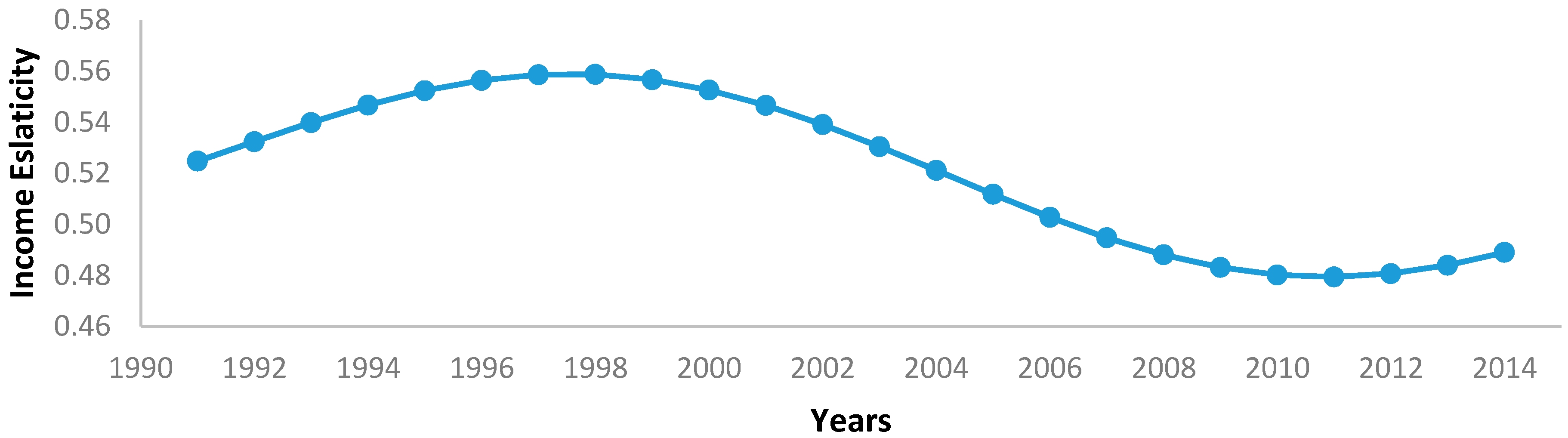
Time-varying income elasticity is found to be positive across the entire time period ranging within the interval [0.48; 0.56]. That is, a 1% change in the income level leads to from 0.48% to 0.56% change in the electricity consumption in the long run. The TVC of income is depicted in Figure 2.
As can be seen from Figure 2, income elasticity demonstrates considerable variation across the time period. Income elasticity was increasing gradually until 1999. It can be explained by the fact that the economy recovered from the recession since 1995 and income increased accordingly. Thus, more income led to more electricity to consume. The coefficient kept decreasing more gradually since 1999 and demonstrated almost constant behavior towards the end of the period 2000–2011. It can be explained by a number of reasons. First, starting in 2000, the government implemented a number of measures, which resulted in an increase in energy, specifically electricity, efficiency and reduction in losses. Second, the coverage area of metric system installation expanded significantly to prevent unnecessary usage of electricity. Third, the electricity tariff was increased by three times in 2007 by the government, which in turn led to less electricity consumption and/or reduction in unnecessary usage of it. Fourth, as the income level was increasing over the period, the sectors of electricity consumption, such as residential and industry, tended to buy energy-efficient technology and appliances. All of the above-mentioned measures are well discussed in [53], among others. Fifth, electricity is the commodity, which consumption is upper bounded. Meaning that if the income level increases continuously it does not necessitate a corresponding increase in the electricity consumption (see [27,31] inter alia). The proliferation era of high technology and electronic devices occurred since 2006 in the advanced economies [22]. It spilled over to Azerbaijan since 2012 due to the lagged catch-up and post financial crisis recovery. The increase in the demand for electronic devices and high technology in all the electricity consumption sectors such as residential, commercial and government services and industry was followed by an increase in electricity consumption.
It is worth noting that the above-mentioned “behavior” of the income elasticity as well as explanations are in line with the findings of [54].
6. Conclusions
The paper investigates the relationship between electricity demand and economic activity, electricity price using the Time-Varying Coefficient cointegration approach in order to capture the time-variant response of electricity demand to income level, which might be caused due to factors such as rapid economic development, experiencing different economic developmental stages for the period of investigation, shocks in the economy (for example, oil shocks), among others.
The empirical estimation of the income elasticity of electricity demand in Azerbaijan shows that there is a considerable variation for the period of investigation, ranging from 0.48 to 0.56. The price elasticity is found to be economically meaningful with an appropriate sign and size, while it is statistically insignificant. The small magnitude (−0.013) of price elasticity can be explained with two factors: electricity is a necessary good and the electricity price in Azerbaijan is centrally regulated.
The findings of the study have some policy implications. We found that income elasticity of the electricity consumption is not constant over time. It implies that policy decisions based on the forecasts or analyses using invariant elasticity should be revised. Another finding is that income elasticity started to increase towards the end of the period. In this regard, decision makers in Azerbaijan should expect more electricity demand by economic agents if income level will rise in the short to medium run. We found that price elasticity of the electricity consumption is inelastic and insignificant. From a policy perspective, it implies that future regulation in electricity tariff would not have a significant impact on the electricity consumption.
Acknowledgments
We are grateful to professors Joon Park and Yoosoon Chang for their very constructive comments. Mikayilov, in particular, thanks them for their continuous support in deeply understanding and application of the TVC approach. The views expressed in this study are those of the authors and do not necessarily represent the views of their affiliated institutions. We are responsible for all error and omissions.
Author Contributions
All authors contributed to the research and the write up of the manuscript equally. In particular, Jeyhun I. Mikayilov worked on the data section, econometric methodology, conducted estimations, while Fakhri J. Hasanov did the literature review and interpretation of the estimation results. Carlo A. Bollino worked on the introduction and theoretical framework and Ceyhun Mahmudlu was responsible for the general style of the paper as well as for the reference list. The conclusion section written by all authors collectively.
Conflicts of Interest
The authors declare no conflict of interest.
References
- Bentzen, J.; Engsted, T. Short-and long-run elasticities in energy demand: A cointegration approach. Energy Econ. 1993, 15, 9–16. [Google Scholar] [CrossRef]
- Reiss, P.; White, M. Household electricity demand, revisited. Rev. Econ. Stud. 2005, 72, 853–858. [Google Scholar] [CrossRef]
- Karimu, A.; Brännlund, R. Functional form and aggregate energy demand elasticities: A nonparametric panel approach for 17 OECD countries. Energy Econ. 2013, 36, 19–27. [Google Scholar] [CrossRef]
- Horowitz, M.J. Changes in electricity demand in the United States from the 1970s to 2003. Energy J. 2007, 28, 93–119. [Google Scholar] [CrossRef]
- Labandeira, X.; Labeaga, J.M.; Lopez-Otero, X. Estimation of elasticity price of electricity with incomplete information. Energy Econ. 2012, 34, 627–633. [Google Scholar] [CrossRef]
- Krishnamurthy, C.K.B.; Kriström, B. A cross-country analysis of residential electricity demand in 11 OECD-countries. Resour. Energy Econ. 2015, 39, 68–88. [Google Scholar] [CrossRef]
- Prosser, R.D. Demand elasticities in OECD: Dynamical aspects. Energy Econ. 1985, 7, 9–12. [Google Scholar] [CrossRef]
- Fell, H.; Li, S.; Paul, A. A new look at residential electricity demand using household expenditure data. Int. J. Ind. Organ. 2014, 33, 37–47. [Google Scholar] [CrossRef]
- Sun, Y.; Yu, Y. Revisiting the residential electricity demand in the United States: A dynamic partial adjustment modelling approach. Soc. Sci. J. 2017, 54, 295–304. [Google Scholar] [CrossRef]
- Flaig, G. Household production and the short- and long-run demand for electricity. Energy Econ. 1990, 12, 116–121. [Google Scholar] [CrossRef]
- Narayan, P.K.; Smyth, R. The residential demand for electricity in Australia: An application of the bounds testing approach to cointegration. Energy Policy 2005, 33, 467–474. [Google Scholar] [CrossRef]
- Arisoy, I.; Ozturk, I. Estimating industrial and residential electricity demand in Turkey: A time varying parameter approach. Energy 2014, 66, 959–964. [Google Scholar] [CrossRef]
- Salisu, A.A.; Ayinde, T.O. Modeling energy demand: Some emerging issues. Renew. Sustain. Energy Rev. 2016, 54, 1470–1480. [Google Scholar] [CrossRef]
- Haas, R.; Schipper, L. Residential energy demand in OECD-countries and the role of irreversible efficiency improvements. Energy Econ. 1998, 20, 421–442. [Google Scholar] [CrossRef]
- Chang, Y.; Martinez-Chombo, E. Electricity Demand Analysis Using Cointegration and Error-Correction Models with Time Varying Parameters: The Mexican Case; Working Paper 2003-08; Department of Economics, Rice University: Houston, TX, USA, 2003. [Google Scholar]
- Terasvirta, T.; Anderson, H.M. Characterizing nonlinearities in business cycles using smooth transition autoregressive models. J. Appl. Econ. 1992, 7, S119–S136. [Google Scholar] [CrossRef]
- Dargay, J.M. Are Price and Income Elasticities of Demand Constant? Working Paper 16; Oxford Institute for Energy Studies: Oxford, UK, 1992. [Google Scholar]
- Stock, J.H.; Watson, M.W. Evidence on structural instability in macroeconomic time series relations. J. Bus. Econ. Stat. 1996, 14, 11–30. [Google Scholar]
- Phillips, P.C.B. Trending time series and macroeconomic activity: Some present and future challenges. J. Econ. 2001, 100, 21–27. [Google Scholar] [CrossRef]
- Lucas, R.R. Econometric policy evaluation: A critique. Carnegie-Rochester Conf. Ser. Public Policy 1976, 1, 19–46. [Google Scholar] [CrossRef]
- Park, J.Y.; Hahn, S.B. Cointegrating regressions with time varying coefficients. Econ. Theory 1999, 15, 664–703. [Google Scholar] [CrossRef]
- Chang, Y.; Kim, C.K.; Miller, J.I.; Park, J.Y.; Park, S. Time-varying Long-run Income and Output Elasticities of Electricity Demand with an Application to Korea. Energy Econ. 2014, 46, 334–347. [Google Scholar] [CrossRef]
- Hasanov, F.J.; Hunt, L.C.; Mikayilov, C.I. Modeling and Forecasting Electricity Demand in Azerbaijan Using Cointegration Techniques. Energies 2016, 9, 1045. [Google Scholar] [CrossRef]
- Hasanov, F.; Hasanli, K. Why had the Money Market Approach been irrelevant in explaining inflation in Azerbaijan during the rapid economic growth period? Middle East. Financ. Econ. 2011, 10, 1–11. [Google Scholar]
- World Bank. Word Development Indicators. Available online: http://www.worldbank.org (accessed on 21 September 2017).
- Vidadili, N.; Suleymanov, E.; Bulut, C.; Mahmudlu, C. Transition to renewable energy and sustainable energy development in Azerbaijan. Renew. Sustain. Energy Rev. 2017, 80, 1153–1161. [Google Scholar] [CrossRef]
- Hasanov, F.J.; Mikayilov, J.I. The impact of age groups on consumption of residential electricity in Azerbaijan. Communist Post-Communist Stud. 2017, in press. [Google Scholar] [CrossRef]
- Dietz, T.; Rosa, E.A. Rethinking the environmental impacts of population, affluence, and technology. Hum. Ecol. Rev. 1994, 1, 277–300. [Google Scholar]
- Dietz, T.; Rosa, E.A. Effects of population and affluence on CO2 emissions. Proc. Natl. Acad. Sci. USA 1997, 94, 175–179. [Google Scholar] [CrossRef] [PubMed]
- Bildirici, M.E.; Kayikci, F. Economic growth and electricity consumption in former Soviet Republics. Energy Econ. 2012, 34, 747–753. [Google Scholar] [CrossRef]
- Klytchnikova, I. Methodology and Estimation of the Welfare Impact of Energy Reforms on Households in Azerbaijan. Ph.D. Thesis, University of Maryland, College Park, MD, USA, 2006. [Google Scholar]
- Azerenerji Joint Stock Company (AJSC). Electricity Forecast Report; Azerenerji: Baku, Azerbaijan, 2009. [Google Scholar]
- Azerenerji Joint Stock Company (AJSC). Electricity Forecast Report; Azerenerji: Baku, Azerbaijan, 2013. [Google Scholar]
- Japan International Cooperation Agency (JICA); Tokyo Electric Power Services Co. (TEPSCO). Study for Electric Power Sector in Azerbaijan; JICA: Tokyo, Japan; TEPSCO: Tokyo, Japan, 2013. [Google Scholar]
- Fichtner. Update of the Power Sector Master Plan of Azerbaijan 2013–2025; Fichtner: Stuttgart, Germany, 2013. [Google Scholar]
- Mercados. Azerenerji Generation and Transmission Master Plan 2010–2025; Fichtner: Stuttgart, Germany, 2010. [Google Scholar]
- Inglesi-Lotz, R. The evolution of price elasticity of electricity demand in South Africa: A Kalman filter application. Energy Policy 2011, 39, 3690–3696. [Google Scholar] [CrossRef]
- Adom, P.K. Time-varying analysis of aggregate electricity demand in Ghana: A rolling analysis. OPEC Energy Rev. 2013, 37, 63–80. [Google Scholar] [CrossRef]
- Chang, H.; Hsing, Y. The demand for residential electricity: New evidence on time-varying elasticities. Appl. Econ. 1991, 23, 1251–1256. [Google Scholar] [CrossRef]
- Engle, R.F.; Granger, C.J. Co-integration and Error Correction: Representation, Estimation and Testing. Econometrica 1987, 55, 251–276. [Google Scholar] [CrossRef]
- International Energy Agency. Energy Statistics. Available online: www.iea.org (accessed on 10 May 2016).
- State Agency of Statistics of Azerbaijan. Available online: http://www.astat.org (accessed on 6 July 2016).
- Dickey, D.; Fuller, W. Likelihood Ratio Statistics for Autoregressive Time Series with a Unit Root. Econometrica 1981, 49, 1057–1072. [Google Scholar] [CrossRef]
- Phillips, P.B.; Perron, P. Testing for Unit Roots in Time Series Regression. Biometrika 1988, 75, 335–346. [Google Scholar] [CrossRef]
- Silk, J.; Joutz, F. Short and long-run elasticities in US residential electricity demand: A co-integration approach. Energy Econ. 1997, 19, 493–513. [Google Scholar] [CrossRef]
- Park, J.Y. Canonical Cointegrating Regressions. Econometrica 1992, 60, 119–143. [Google Scholar] [CrossRef]
- Park, J.Y. Testing for unit roots and cointegration by variable addition. In Advances in Econometrics; Rhodes, G.F., Fomby, T.B., Eds.; JAI Press: Greenwich, UK, 1990; pp. 107–133. [Google Scholar]
- MacKinnon, J. Critical Values for Cointegration Test. In Long-Run Economic Relationships; Engle, R., Granger, C., Eds.; Oxford University Press: Oxford, UK, 1991. [Google Scholar]
- Zivot, E.; Andrews, D. Further evidence of great crash, the oil price shock and unit root hypothesis. J. Bus. Econ. Stat. 1992, 10, 251–270. [Google Scholar]
- Johansen, S. Statistical analysis of cointegration vectors. J. Econ. Dyn. Control 1988, 12, 231–254. [Google Scholar] [CrossRef]
- Johansen, S.; Juselius, K. Maximum likelihood estimation and inference on cointegration with applications to the demand for money. Oxf. Bull. Econ. Stat. 1990, 52, 169–210. [Google Scholar] [CrossRef]
- Pesaran, H.M.; Shin, Y. An Autoregressive Distributed Lag Modeling Approach to Cointegration Analysis. In Econometrics and Economic Theory in the 20th Century: The Ragnar Frisch Centennial Symposium; Strom, S., Ed.; Cambridge University Press: Cambridge, UK, 1999. [Google Scholar]
- Opitz, P.; Kharazyan, A.; Pasoyan, A.; Gurbanov, M.; Margvelashvili, M. Sustainable Energy Pathways in the South Caucasus: Opportunities for Development and Political Choices; South Caucasus Regional Office of the Heinrich Boell Foundation: Tbilisi, Georgia, 2015. [Google Scholar]
- Chang, Y.; Choi, Y.; Kim, C.S.; Miller, J.I.; Park, J.Y. Disentangling temporal patterns in elasticities: A functional coefficient panel analysis of electricity demand. Energy Econ. 2016, 60, 232–243. [Google Scholar] [CrossRef]
Figure 1.
Graphs of the logarithmic forms of the variables and their growth rates.
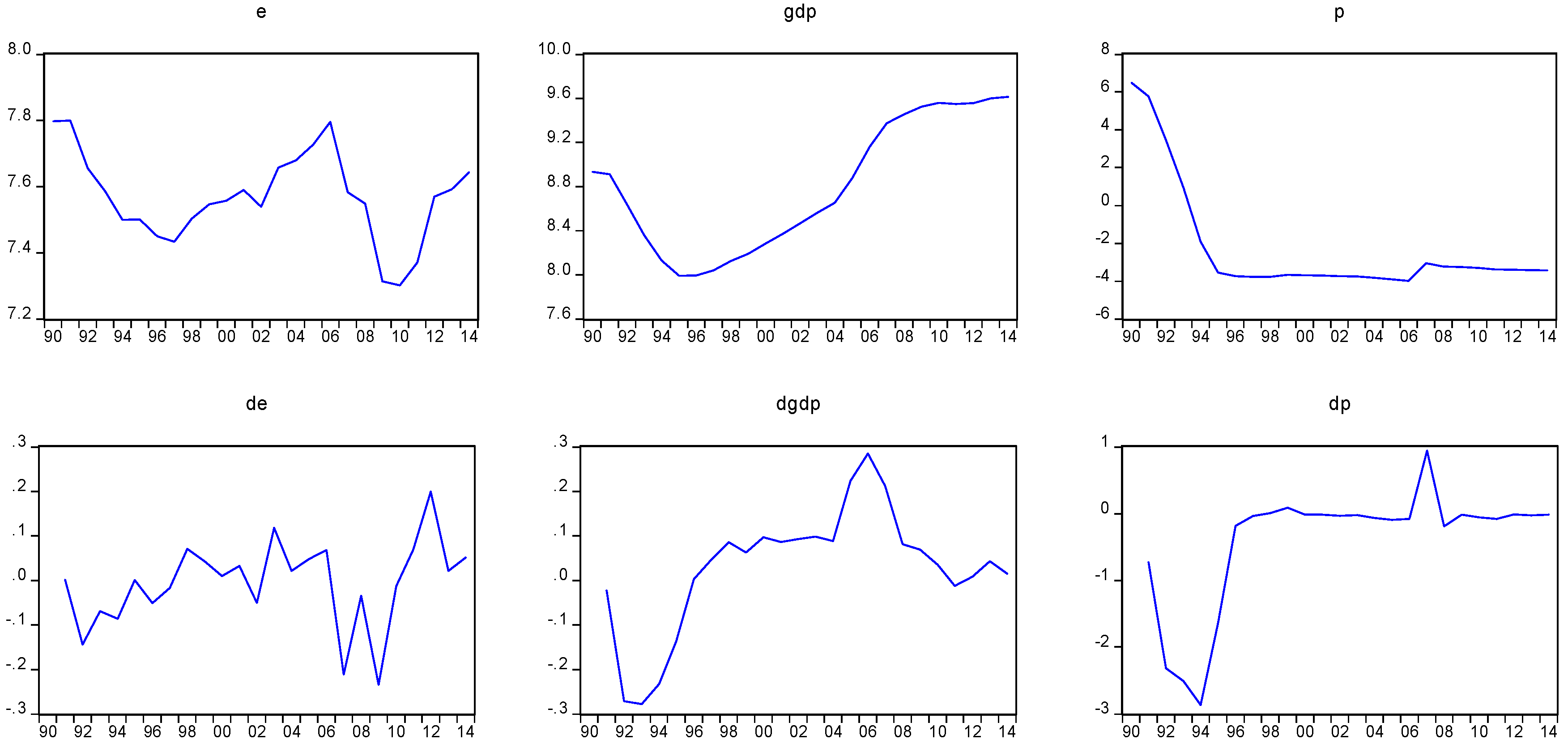
Figure 2.
Time-varying income elasticity.


Table 1.
The Unit Root test results.
| Variable | The ADF Test | The PP Test | |||||||
|---|---|---|---|---|---|---|---|---|---|
| Test Value | C | t | None | k | Test Value | C | t | None | |
| e | −3.787 ** | x | 2 | −2.446 | x | ||||
| p | −7.794 *** | x | 1 | −2.990 | x | ||||
| gdp | −6.379 *** | x | 1 | −2.736 | x | ||||
| e | −3.846 *** | x | 0 | −3.909 *** | x | ||||
| p | −1.581 | x | 0 | −1.644 * | x | ||||
| gdp | −3.436 ** | x | 1 | −1.567 | |||||
Notes: ADF and PP denote the Augmented Dickey–Fuller and Phillips–Perron tests respectively. Maximum lag order is set to two and optimal lag order (k) is selected based on Schwarz criterion in the tests; ***, ** and * indicate rejection of the null hypotheses at the 1%, 5% and 10% significance levels, respectively; denotes the first difference operator; The critical values for the tests are taken from [48]. None means that neither intercept nor trend is included in test equation. Note again that final UR test equation can include one of the three options: intercept (C), intercept and trend (t) and none of them (None). x indicates that the corresponding option is selected in the final UR test equation.
Table 2.
Results of the test for joint significance of coefficients and cointegration test.
| Test for Joint Significance of Time-Varying Coefficients | Variable Addition Test | ||||||
|---|---|---|---|---|---|---|---|
| Test statistics | 1% CV | 5% CV | 10% CV | Test statistics | 1% CV | 5% CV | 10% CV |
| 44.43 | 15.09 | 11.07 | 9.24 | 59.89 | 13.18 | 9.49 | 7.78 |
Notes: The left-hand side of the table demonstrates results of the joint significance test of time-varying coefficients, namely λ1= λ2= λ3 = 0 in order to test whether or not the income elasticity is fixed or time-varying. The right-hand side of the table shows the results of VAT cointegration test.
Table 3.
Results of the Time-Varying Coefficient model.
| Statistics | Coefficient | Parameters of the Time-Varying Income Coefficient | ||||
|---|---|---|---|---|---|---|
| Heading | τ | β | λ0 | λ1: | λ2: | λ3: |
| estimates | 3.088 | −0.013 | 0.537 | −0.065 | −0.006 | 0.032 |
| t-values | 2.828 | −0.457 | 4.224 | −1.765 | −0.590 | 2.587 |
| p-values | 0.011 | 0.653 | 0.000 | 0.096 | 0.563 | 0.019 |
Note: τ and β denote intercept and price elasticity, respectively.
© 2017 by the authors. Licensee MDPI, Basel, Switzerland. This article is an open access article distributed under the terms and conditions of the Creative Commons Attribution (CC BY) license (http://creativecommons.org/licenses/by/4.0/).
Share and Cite
MDPI and ACS Style
Mikayilov, J.I.; Hasanov, F.J.; Bollino, C.A.; Mahmudlu, C. Modeling of Electricity Demand for Azerbaijan: Time-Varying Coefficient Cointegration Approach. Energies 2017, 10, 1918. https://doi.org/10.3390/en10111918
AMA Style
Mikayilov JI, Hasanov FJ, Bollino CA, Mahmudlu C. Modeling of Electricity Demand for Azerbaijan: Time-Varying Coefficient Cointegration Approach. Energies. 2017; 10(11):1918. https://doi.org/10.3390/en10111918
Chicago/Turabian StyleMikayilov, Jeyhun I., Fakhri J. Hasanov, Carlo A. Bollino, and Ceyhun Mahmudlu. 2017. "Modeling of Electricity Demand for Azerbaijan: Time-Varying Coefficient Cointegration Approach" Energies 10, no. 11: 1918. https://doi.org/10.3390/en10111918
Note that from the first issue of 2016, this journal uses article numbers instead of page numbers. See further details here.