Internal Combustion Engine Model for Combined Heat and Power (CHP) Systems Design


Aeronautical and Automotive Engineering, Loughborough University, Leicestershire LE11 3TU, UK
*
Author to whom correspondence should be addressed.
Energies 2017, 10(12), 1948; https://doi.org/10.3390/en10121948
Submission received: 19 August 2017
/
Revised: 20 November 2017
/
Accepted: 21 November 2017
/
Published: 25 November 2017
(This article belongs to the Section L: Energy Sources)
Abstract
:A model based, energy focused, quasi-stationary waste heat driven, internal combustion engine (ICE) centred design methodology for cogeneration (heat and electricity) systems is presented. The developed parametric model could be used for system sizing, performance evaluation, and optimization. This paper presents a systematic approach to model the behaviour of the CHP system using heat recovery prediction methods. The modular, physics based modelling environment shows the power flow between the system components, with a special emphasis on the ICE subsystems, parameter identification, and model validation.
1. Introduction
Combined heat and power (CHP) or cogeneration technology involves the generation of readily useable heat and power from a single fuel source [1,2,3,4,5]. It most commonly involves the operation of a prime mover such as an internal (spark ignited & compression ignited reciprocating engines, gas turbines) or external (Stirling, Rankine) combustion engine, and utilizes the waste heat of the power producing cycle for heating purposes, thus increasing the overall efficiency of the application.
Due to the potential for resource and environment conservation, as well as the desire for power autonomy, the combined heat and power (CHP) market is expanding [6] and is starting to penetrate the small residential sector, for the scale of which (electrical capacity lower than 10 kWe), ICE based micro-CHP systems are currently the most marketable of the available micro-CHP types due to sharing an established, mature, highly reliable technology, while at the same time being characterized by low purchase and maintenance costs [1,2,3,7,8,9,10,11,12,13]. While Compression Ignition (CI) engines enjoy a widespread proliferation in the role of larger stationary power plants due to their associated advantages, such as a high fuel conversion efficiency and durability, the fact that Natural Gas (NG) is readily available to households through transmission pipeline networks, the environmentally friendly nature of the fuel, as well as the low cost and effort adaptability of Spark Ignited (SI) engines to run on Natural Gas has made small NG fuelled SI engines the technology of choice for powering the majority of currently available ICE based micro-CHP units. The above, when combined with the widespread usage of simulation tools for CHP system research, design, and selection, as well as the special nature of cogeneration technology, have created the need for fast running mathematical models of spark ignited internal combustion engines (SI ICE ) that predict both power and waste heat components. As a response, several researchers have developed a number of quasi-stationary ICE and CHP models.
Voorspools and D’haeseleer [14] have shown that the transient behaviour of engine fuel conversion efficiency is fast enough to be neglected in micro-CHP simulation applications, and this is reflected in the observation that the majority of CHP models that are encountered in literature are of the quasi-stationary type. Caresana et al. [7], made use of a lookup table based ICE modelling layout in which, one lookup table returned fuel flow, and another table returned the exhaust heat as fraction of chemical power inlet for given combinations of engine torque and speed. On the other hand, the parametric CHP model that is available in the ESP-r building simulation software library, and that is used in a number of studies on micro-CHP performance [2,15,16], is based on a polynomial fit. Under this modelling technique, the CHP system is modelled as one single unit and the model dependent variables, such as the Brake Specific Fuel Consumption, the Electrical Efficiency, and the Heat to Power Ratio are calculated as polynomial functions of part load ratio. Another encountered polynomial model was used by Cho et al. [17], who calculated system electrical efficiency as a function of the electrical output of the generator set, while they assumed coolant and exhaust heat to be constant fractions of 0.3 of the chemical power inlet.
On the other hand, the engine thermal response is much slower, and for this reason, it is often included in cogeneration system models. In one study, thermal transient behaviour of the engine is described by means of polynomial functions of time elapsed after shut down [2]. Kelly et al. [15] used an engine model with a lumped capacitance transient thermal model with one node representing the engine and the heat exchanger masses, and another node representing the water mass. In terms of the transient behaviour of the exhaust temperature, Zavala et al. [18], found in their experimental data that it can be adequately described by 1st order linear transfer functions, with AFR, spark timing, and engine speed as their main model inputs.
Since the majority of CHP modelling applications involves the study of a particular CHP system design, or the use of an averaged map based engine model on a CHP model, the encountered layouts as described above have been found to be very well suited for most studies. In some cases though, especially when the model is to be used in heat recovery system design applications, separating the engine from the heat exchanger performance, while at the same time retaining engine model scalability, can be a desirable combination of model characteristics.
The main aim of this document is the development of an SI ICE model layout for use in CHP sizing and design applications whose special nature may require that the engine model incorporates the behaviour of all of the necessary power components, temperatures, and flow rates for use with a heat recovery system model, while at the same time being characterized by an increased scalability and connectivity to heat recovery component models, simplicity, and a low computational load.
The structure of this paper is as follows: First, Section 2 presents the structure of the system model and the mathematical relationships that are used to describe the flow of power between the model components. Section 3 describes the procedure that is followed to collect the necessary experimental data and identify the required model parameters. The developed model is then simulated and validated in Section 4, while a discussion on simulation results takes place in Section 5. Finally, Section 6 contains the conclusions of this study.
2. System Model
The communication layout of the developed model will be power based, as in such a configuration; power can be used to connect individual subsystems and phenomena that handle energy on multiple domains. In addition, contrary to most existing lookup table based engine models whose main maps include parameters that are directly linked to mechanical power and fuel consumption, the developed model will follow a reverse logic—not unlike the general layout presented by Heß et al. [19]—by means of which, specific sub-models and their respective lookup tables provide the rates of the generated waste heat components, whose values are then subtracted from the energy input rate to provide the mechanical power output .
Heat inlet from the fuel is released in the combustion chamber at a rate , and part of it is converted to mechanical power output . Exhaust heat is carried by the high temperature exhaust gases at a rate . Convective heat flows from the hot cylinder content to the colder engine mass at a rate and is finally released into the engine coolant as well as the engine surroundings by means of conduction, convection, and radiation. Heat that is generated by friction at a rate is dissipated by the engine oil [20,21]. This configuration gives the researcher the ability to fine-tune the three different waste heat sub-models to better approximate a given engine. A simplified schematic of the developed model analysing its layout and main constituent subsystems is shown in Figure 1.
The PI controller uses the set speed and the actual speed to set the value of the control variable volumetric efficiency . The physical limits of the system are defined by a saturation filter. In order for the engine model to be generally applicable, and for the sake of simplicity, fluid densities and specific volumes for atmospheric pressure , rather than for the manifold pressure, are used due to the fact that the pressure characteristics of the manifold may vary significantly throughout the engine operating range and from one engine type to another. The following assumptions can be made of the model and these are generally true for commercially available, calibrated, healthy running SI engines:
- The charge air fuel ratio (AFR) is assumed to always be stoichiometric.
- Spark timing is assumed to occur at maximum brake torque (MBT) for all of the operating points.
In addition, the amount of fuel that is present in the charge is assumed to have completely evaporated before it enters the cylinder, and thus, in the case of port injected engines, the volumetric efficiency during the parameter estimation phase is calculated from:
where , the volumetric flow rate of the experimentally acquired charge, the theoretical swept volumetric flow rate, , and the volumetric flow rates of the air charge and the evaporated fuel, respectively, all under atmospheric conditions in , the engine displacement in , the mass flow of fuel, , and the specific volumes of the fuel vapour and air, respectively, at atmospheric conditions.
Since the rate of flow of exhaust heat is a function of the exhaust temperature and the exhaust mass flow rate (equal to the charge mass flow rate ), the calculation of the exhaust mass flow rate is an important element of the functionality of the model. Under the above assumptions, the mass flow rate of an air-fuel mixture (charge mass flow rate) of a known ratio for a given combination of , is calculated from:
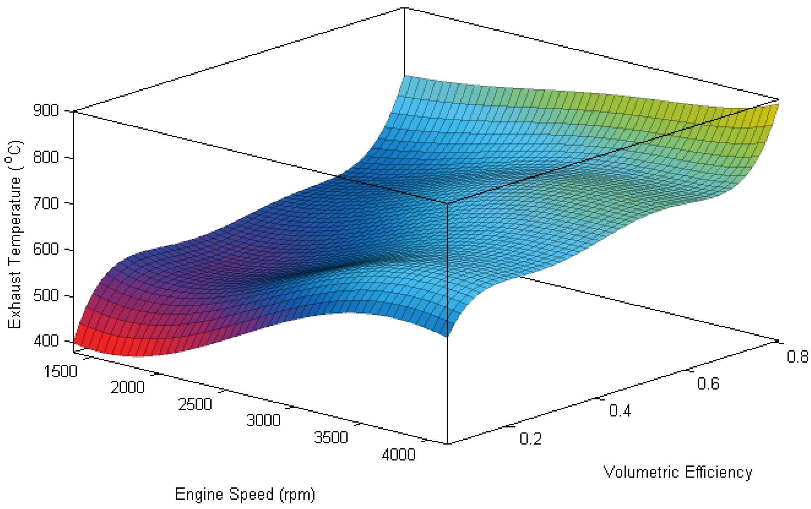
Experience has shown that exhaust temperature may vary significantly throughout the operating range of an internal combustion engine. In the case of spark ignited (SI) engines, exhaust temperature for higher loads lies in the region of 600 °C, and in some cases, may even reach 900 °C, while at idle, it lies in the region of 300 °C, [22], and according Zavala et al. [18], engine speed has a stronger influence than the air mass inlet rate on exhaust temperature. At the time of this writing, the most relevant study on the behaviour of the exhaust temperature of SI engines has been found to have been conducted by Eriksson [23], who based on results from crank angle based combustion models assumed a linear dependence of the exhaust temperature on the exhaust mass flow rate. As the experiments of Section 3 indicate a strong correlation between engine speed and engine volumetric efficiency, in the current document, the exhaust temperature will be calculated as a function of engine speed and engine volumetric efficiency. The sequence of calculations of the power component calculator of the developed engine model is illustrated in the diagram of Figure 2. Once the exhaust outlet temperature is provided from the exhaust temperature map for a given combination of , , the specific enthalpy of the exhaust gas at this temperature is known. Since the specific enthalpy of the exhaust under ambient temperature is also known, the rate of exhaust heat flow is calculated from:
Heat ratio is a size-independent representation of the rate of convective heat transfer that is used by the developed model. The model uses the calculated rate of exhaust heat flow and the heat ratio map to calculate the rate of convective heat transfer or a given combination of , :
links to , which makes model scaling a simple task, since engine displacement defines the rate of exhaust heat flow , the heat inlet rate , and the rate of heat generated by friction (discussed below). In turn, defines for a given operating point.
Using the quadratic fit of as a function of engine speed from Ferguson et al. [20], the rate of generation of heat from friction (engine displacement in ) is calculated from:
For a fuel lower heating value, , the rate of energy that enters the engine in the form of fuel chemical power is calculated from:
The engine mechanical power output is now calculated from:
3. Parameter Identification
The main maps of the model that calculates the exhaust temperature and the heat ratio , both as functions of the engine speed and the engine load will be constructed. A series of tests have been performed on an SI direct injection engine using a transient engine test cell. The engine specifications and Engine Control Unit (ECU) settings used for in the tests are presented in Table 1.
Set speed was varied from 1500 rpm to 4000 rpm in 500 rpm increments. For each set speed value, α was varied from 20% to 100% of maximum throttle angle in increments of 10%. The exhaust temperature, the fuel mass flow rate, and the engine torque were directly measured. All of the tests were carried out on the same day in order to reduce the potential for introduction of error due to inconsistent conditions to the set of recorded data.
The coefficients of 5th order polynomial fits performed on the acquired datasets of and of the tested engine, whose surface plots are shown in Figure 3 and Figure 4, are provided in Appendix A Table A1 to be used in a polynomial of the general form Equation (8).
4. Simulation and Validation
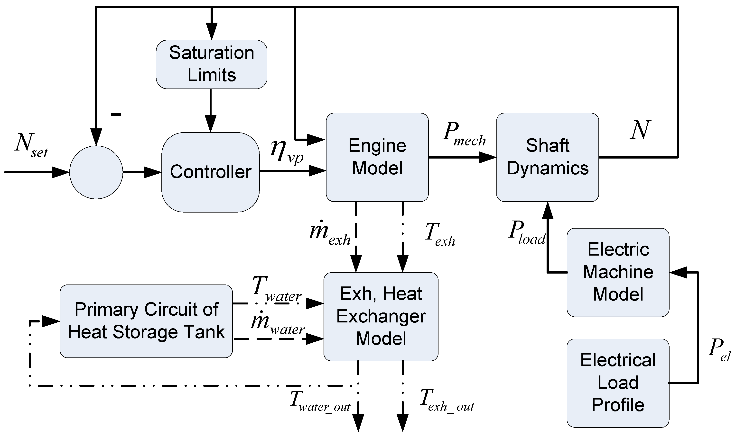
In order to showcase the operation of the engine model that was developed in the previous sections within a CHP application, the engine model is connected to a higher level cogeneration model whose block diagram is shown in Figure 5. A simple four-dimensional (4-D) map based heat exchanger model is connected to and receives input signals from the engine model, as well as from the primary circuit of a thermal storage tank model. The heat exchanger model input signals are the exhaust mass flow rate and temperature from the engine model, and the water mass flow rate and inlet temperature from the thermal storage tank primary circuit . The heat exchanger output signals are the two outlet temperatures.
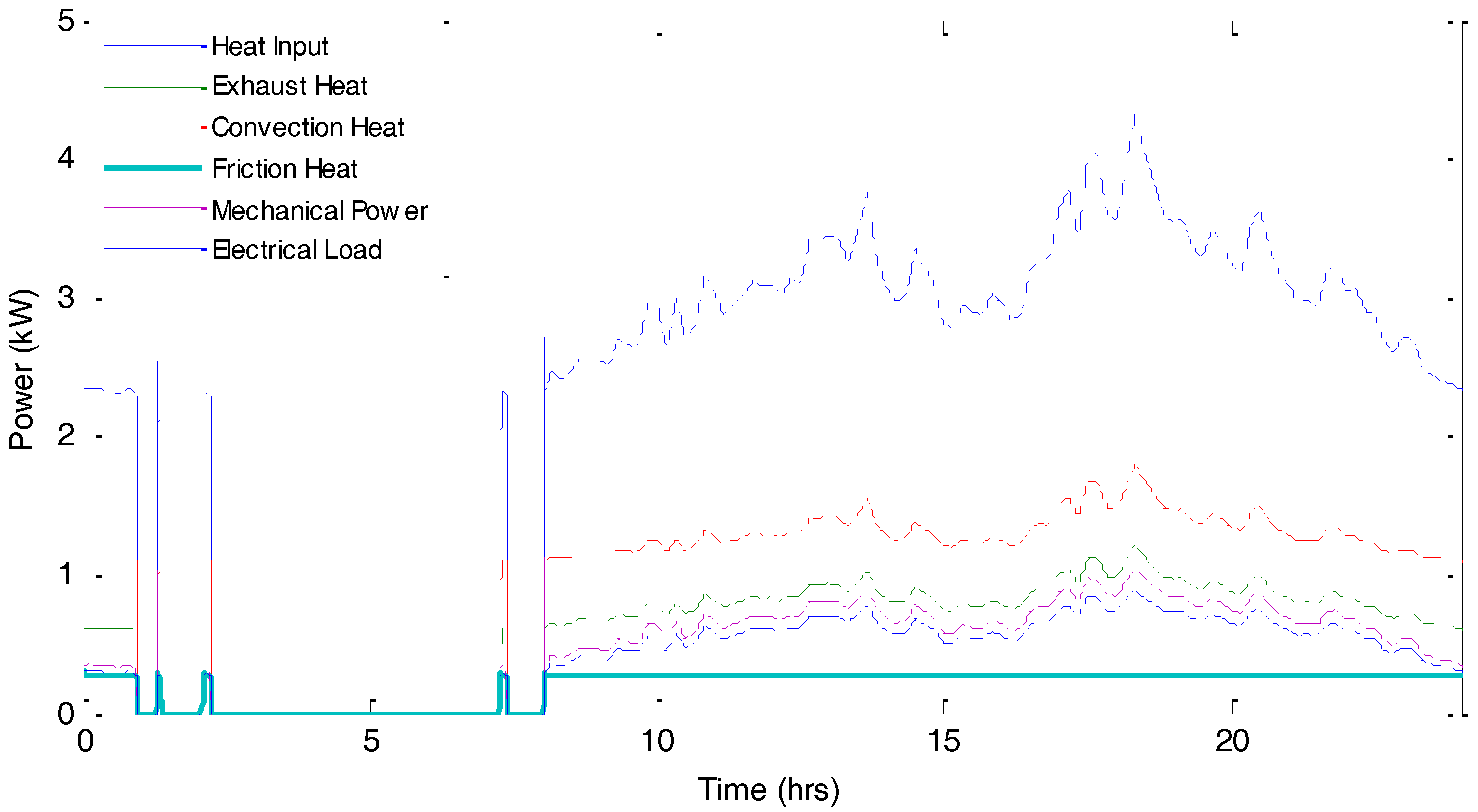
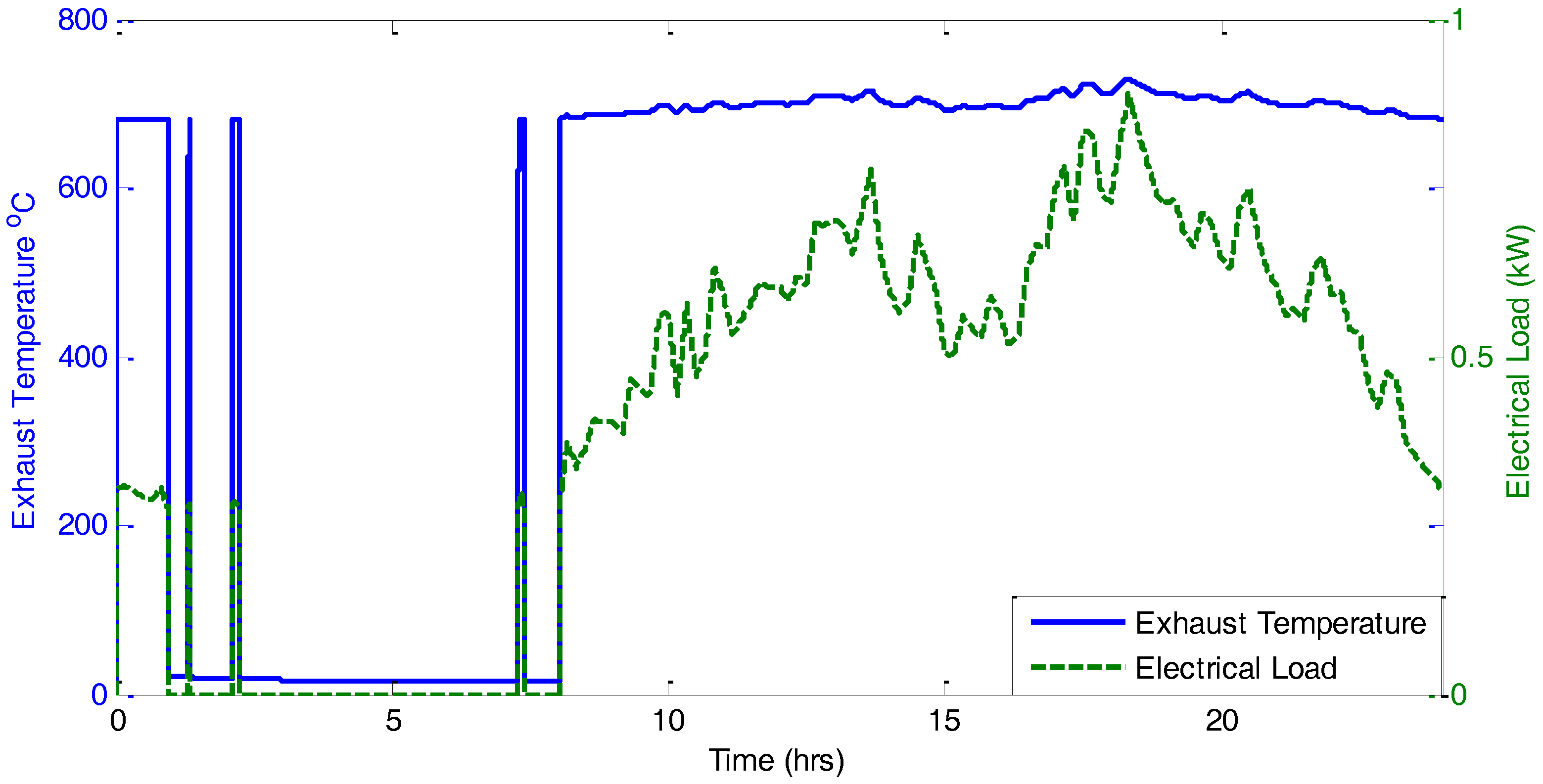
In the simulation study, the engine speed was kept constant with varying electrical load demand for the duration of a day (24 h) at a simulation step of 1 s. The electrical load profile of a mid-terraced house during a typical January day, as found in [24], is used as the system electrical load. Following the simulation, the plots of the different estimated power components flowing through the engine model and the system electrical load profile can be seen in Figure 6. The time intervals during which all of the components equal 0, correspond to the system that is being switched off. The distribution of energy flow rate between the modelled energy components can be observed to vary with load as the distance between each curve is not proportional to the magnitude of the heat input curve along the simulation duration. This behaviour is particularly observable when the mechanical power and rate of the exhaust heat flow plots are compared. While the rate of exhaust heat flow for low electrical loads has a noticeably higher magnitude than the produced mechanical power, for higher loads the rate of exhaust heat flow and power output magnitudes are in close proximity. This behaviour is not surprising as it reflects the higher engine conversion efficiency that is usually observed at higher engine loads. Due to a constant speed operation, the calculated rate of heat generated from friction remains constant. Similarly, the effects of load fluctuation on the predicted exhaust temperature can be observed on the plot of Figure 7 where the exhaust temperature predicted by the system simulation as discussed above is plotted against time, while the electrical load profile is located on the same graph and measured by the right y-axis. Again, the model is found to calculate exhaust temperature values that come to a general agreement with the measured values and whose behaviour follows the observations that were made on the experimental data showing higher loads leading to higher predicted temperatures, and vice versa.
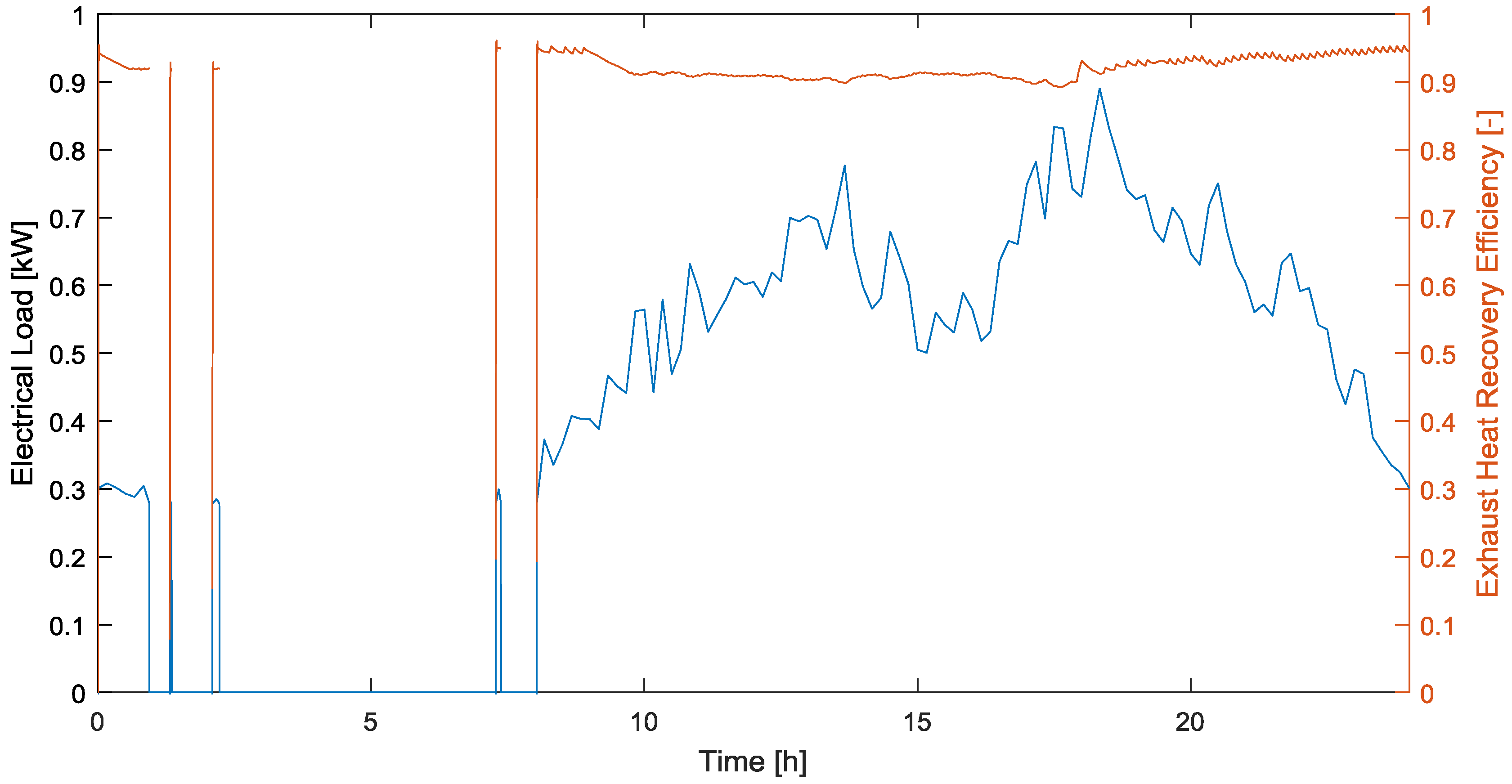
By inspecting the profile of the heat recovery efficiency curve of Figure 8, it can be observed that the model behaves as expected, being affected by the inlet conditions of the heat exchanger subsystem. It can be seen that the instantaneous heat recovery efficiency tends to be higher for low load than for high load conditions. A maximum heat recovery efficiency of 0.95 has been observed for a low electrical load of 0.3 kW to 0.35 kW. On the other hand, a minimum heat recovery efficiency of 0.89 is observed for a high electrical load of 0.83 kW due to an increase in exhaust temperature and mass flow rate. Thus, the minimum heat recovery efficiency is 6.3% lower than the observed maximum heat recovery efficiency. Depending on model specifications, the inclusion of this level of accuracy may be required by the heat recovery model and under these circumstances; an engine model layout as developed in the current document can be the solution in supplying a heat exchanger model with the necessary inputs.
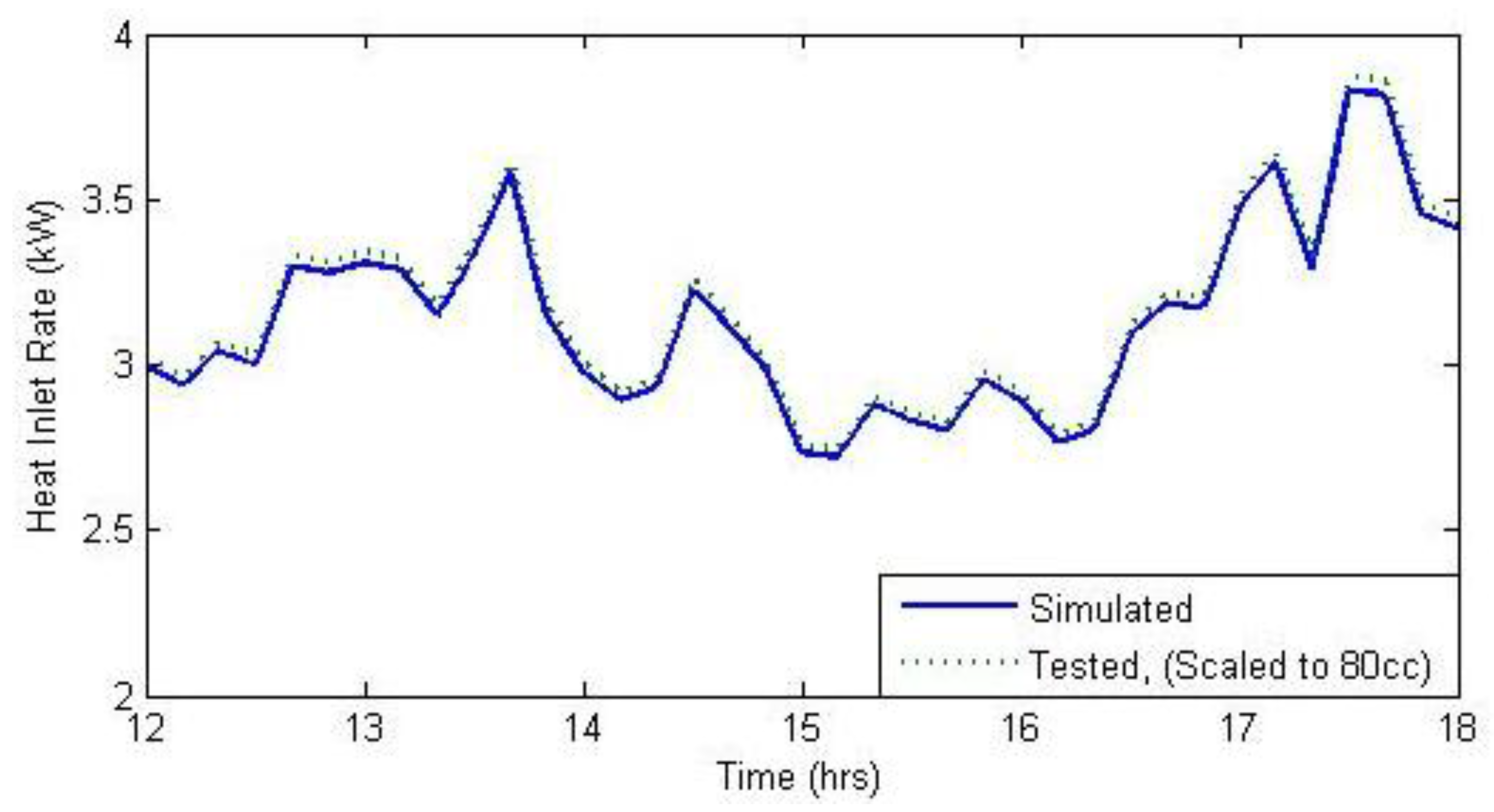
The engine model will be validated in terms of the rate of fuel consumption, as well as the observed exhaust temperature for meeting a certain electrical demand profile. As can be seen in Figure 9, the plotted line of the simulated chemical power inlet exhibits a shape and magnitude that is very similar to the experimentally obtained line (scaled down to 80 cc). The plot of the simulated chemical power inlet remains below the experimental curve for the complete duration of the test. One may observe in Figure 10 that the relative error of the model is rather low, ranging between −0.8% and −1.4% with the contour of the line corresponding to changes in engine load.
Similarly, the degree to which the developed model predicts the exhaust temperature may be observed in Figure 11, where the exhaust temperature profile recorded during the drive cycle phase of the engine test, and the exhaust temperature predicted by the model for the same load are plotted against time. The difference between the two lines ranges between 3 °C and 5 °C, with the simulated line being above the measured temperature curve throughout the duration of the test. A difference of 5 °C for temperatures positioned around the 700 °C mark translate to a relative error of less than 1% when a reference point of 25 °C is considered.
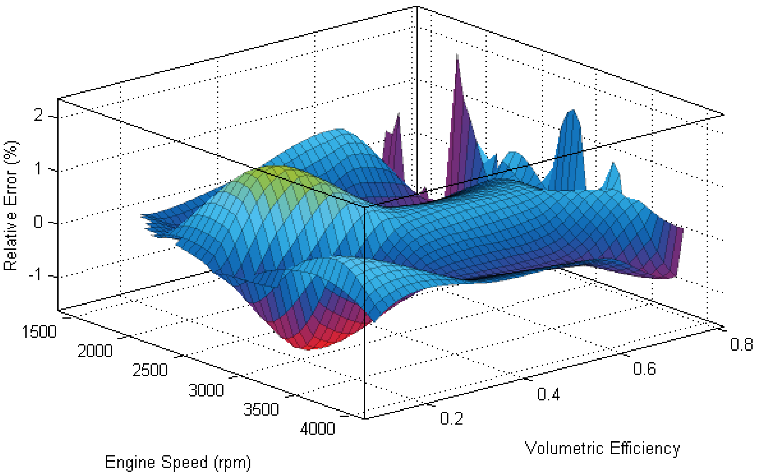
The difference between the plots of Figure 11 can be interpreted through the observation of the relative error surface plot of Figure 12, in which, the relative error of the predicted exhaust temperature is plotted against engine speed and volumetric efficiency. It can be observed that the relative exhaust temperature error ranges between −2% and +2% throughout the complete operating range of the engine. To ensure a fuel efficient operation, the engine was held at a constant synchronous speed of 3000 rpm, and the minimum electrical output of the generator was restricted to 40% of its maximum electrical output. As the engine model was simulated over a map region that is characterized by a low and positive relative exhaust temperature error, the relative error of the simulation remained positive and below 1% throughout the whole duration of the tests.
5. Design and Analysis
The observations that were made in Section 4 regarding the behaviour of the developed engine model come to an agreement with generally established knowledge on the behaviour of spark ignited internal combustion engines, as well as the engine behaviour recorded in the collected engine data, the collection procedure of which is described in Section 3.
The distribution of the different power components that are calculated by the engine model exhibits a behaviour that is quantitatively and qualitatively very similar to that encountered in the tested engine. As expected, the fraction of the inlet chemical power that is converted to mechanical power output (fuel conversion efficiency) at lower loads is low when compared to the fractions of that end up to become the engine main waste heat components. At higher loads, the mechanical power accounts for a greater proportion of the inlet chemical power than in the case of low loads, and this translates to an increase in fuel conversion efficiency. In addition, the proportion each waste heat component accounts for relative to the chemical power inlet varies with load, and depending on the waste heat recovery configuration, this may cause a variation in the system overall fuel utilization efficiency as the engine speed and load varies.
The predicted exhaust temperature exhibits behaviour that is very close to the recorded profile. As in the case of the tested engine, the predicted exhaust temperature is affected by both engine speed and load with speed having a considerably stronger influence on the exhaust temperature magnitude than engine load.
In terms of the degree to which the fitted model of Appendix A Table A1 predicts the magnitude of engine measured outputs accurately, the model validation phase of Section 4 showed a high proximity of the simulation results to the measured data. The relative error of the exhaust temperature fit prediction has been found to be less than 1% when simulated under the engine drive cycle. For the same tests, the relative error of the required chemical power inlet for the same load profile remained between −0.7% and 1.4% throughout the whole simulated period. The strong accuracy of the predicted values can be attributed to the high coefficients of covariance of the 5th order fits of and , which were carried out with the use of Matlab SFTOOL (R2013b, The MathWorks, Natick, MA, USA) to be 0.9959 and 0.9881, respectively. Another potential factor that may have contributed to such low relative errors is the fact that all of the tests were carried out on the same day, which assured that the testing conditions were kept as constant and controlled as possible. While a test performed during a different day of the year may give relative errors of a higher magnitude, the very low errors encountered under testing indicate that the fitted model is adequate for the purpose of modelling and simulating ICE based cogeneration systems, provided that no dramatic changes are made in the engine running conditions, such as in the case of operating under a very low barometric pressure due to high altitude.
6. Conclusions
A method to construct quasi-stationary SI ICE models for use as a subsystem in cogeneration models is presented. The model includes the mechanical power and conversion efficiency aspect of the energy flow, but also the various waste heat components and the exhaust mass flow rate and temperature. Model scalability and connectivity were also considered as characteristics of great importance.
In order to generate the model maps, a series of engine tests have been carried out. By inspecting measured exhaust temperature plots for different engine loads and speeds, a strong dependence of the exhaust temperature, on the engine speed, and the engine volumetric efficiency has been observed. In addition, it is common knowledge that the heat exchanger waste heat recovery efficiency is heavily dependent on fluid inlet conditions. For these reasons, an exhaust temperature model as a function of engine speed and engine volumetric efficiency has been developed. Representing load with volumetric efficiency and mapping the rate of flow of convective heat as a fraction of the rate of flow of the exhaust heat ensures the scalability of the model. The rate of flow of convective heat as a fraction of the rate of flow of the exhaust heat has been named heat ratio () for the ease of documentation. Polynomial surface fits of the exhaust temperature and heat ratio as functions of engine speed and volumetric efficiency of 5th order were performed and the resulting coefficients are included in this document, thus providing the reader with a ready to run engine model. Although quasi-stationary in nature, this layout, if necessary, allows for the incorporation of dynamic behaviour to some extent into the various power components by means of using transfer functions with appropriately tuned coefficients that are dedicated to a respective power component.
The resulting engine model was simulated in tandem with a map based heat exchanger model. The engine model was found to be more than adequate in predicting the measured engine outputs, and easy to connect to a higher level CHP model, thus proving the usefulness of the concept. It is therefore safe to conclude that the developed model is successful in predicting the distribution of all the power components for different speeds and engine loads accurately, while at the same time being easy to scale, and to connect to peripheral components that operate in different energy domains. The most important family of components that can easily be connected to the developed engine model are models of heat recovery equipment whose inlet conditions affect their performance. Due to the above, the developed engine modelling layout can be characterized as an attractive alternative for use in cogeneration simulation applications.
Author Contributions
60% of the work was carried out by Nikolaos Kalantzis, 20% of the work was carried out by Antonios Pezouvanis, 20% of the work was carried out by Kambiz M. Ebrahimi.
Conflicts of Interest
The authors declare no conflicts of interest.
Nomenclature
| Ambient atmospheric temperature | |
| Heat inlet rate from fuel to the engine | |
| Mechanical power output | |
| Exhaust heat rejection rate | |
| Rate of heat rejection through convection from cylinder content to cylinder walls | |
| Exhaust mass flow rate | |
| Air mass flow rate | |
| Fuel mass flow rate | |
| Exhaust temperature | |
| Set engine speed | |
| Engine speed | |
| Mechanical power load acting on the shaft | |
| Engine volumetric efficiency | |
| Ambient pressure | |
| Stoichiometric air to fuel ratio | |
| Volumetric flow rate of vaporized fuel at atmospheric conditions | |
| Specific volume of vaporized fuel at atmospheric conditions | |
| Volumetric flow of air at atmospheric conditions | |
| Specific volume of air at atmospheric conditions | |
| Swept volume rate | |
| Engine displacement | |
| Mass flow rate of charge | |
| Exhaust enthalpy under outlet temperature | |
| Exhaust enthalpy under ambient temperature | |
| Heat ratio | |
| Lower heating value of fuel | |
| Water inlet temperature (Heat exchanger) | |
| Water mass flow rate (Heat exchanger) | |
| Water outlet temperature (Heat exchanger) | |
| Exhaust outlet temperature (Heat exchanger) | |
| Electrical power load placed on the electric machine |
Appendix A

Table A1.
Coefficients of the 5th order polynomial surface fits on and
| 181 | −15.26 | |
| −0.01864 | 0.03765 | |
| 9717 | −62.01 | |
| −0.0002382 | −2.308 × 10⁻⁵ | |
| −2.664 | −0.01654 | |
| −4.732 × 10⁴ | 359.6 | |
| 2.091 × 10⁷ | 4.749 × 10⁹ | |
| 0.0004299 | 4.275 × 10⁻⁵ | |
| 9.603 | −0.2169 | |
| 1.034 × 10⁵ | −396.1 | |
| −5.329 × 10⁻¹¹ | −1.954 × 10⁻¹³ | |
| −4.319 × 10⁻⁸ | −1.029 × 10⁻⁸ | |
| −0.001427 | 1.043 × 10⁻⁶ | |
| −8.814 | 0.3173 | |
| −1.131 × 10⁵ | −19.82 | |
| 4.266 × 10⁻¹⁵ | −2.644 × 10⁻¹⁷ | |
| 6.416 × 10⁻¹² | 7.893 × 10⁻¹³ | |
| 3.797 × 10⁻⁸ | 1.077 × 10⁻⁹ | |
| 0.0008733 | −5.83 × 10⁻⁶ | |
| 2.013 | −0.1529 | |
| 4.992 × 10⁴ | 176 | |
| 0.9959 | 0.9881 |
References
- Onovwiona, H.; Urgusal, V. Residential cogeneration systems: Review of the current technology. Renew. Sustain. Energy Rev. 2006, 10, 389–431. [Google Scholar] [CrossRef]
- Onovwiona, H.I.; Urgusal, V.I.; Fung, A.S. Modelling of internal combustion engine based systems for residential applications. Appl. Therm. Eng. 2007, 27, 848–861. [Google Scholar] [CrossRef]
- Aliabadi, A.A.; Thomson, M.J.; Wallace, J.S. Efficiency analysis of natural gas residential micro-cogeneration systems. Energy Fuels 2010, 24, 1704–1710. [Google Scholar] [CrossRef]
- Angrisani, G.; Roselli, C.; Sasso, M. Distributed microtrigeneration systems. Prog. Energy Combust. Sci. 2012, 38, 502–521. [Google Scholar] [CrossRef]
- Canova, A.; Cavallero, C.; Freschi, F.; Giaccone, L.; Repetto, M.; Tartaglia, M. Comparative economical analysis of a small scale trigenerative plant: A case study. In Proceedings of the Industry Applications Conference, 2007 42nd IAS Annual Meeting, New Orleans, LA, USA, 23–27 September 2007. [Google Scholar]
- Sicre, B.; Buhring, A.; Platzer, B.; Hoffmann, K.H. Energy and cost assessment of Micro-CHP plants in high performance residential buildings. In Proceedings of the ECOS 2005, the 18th International Conference on Efficiency, Cost, Optimization, Simulation, and Environmental Impact of Energy Systems, Trondheim, Norway, 20–22 June 2005. [Google Scholar]
- Caresana, F.; Brandoni, C.; Feliciotti, P.; Bartolini, C.M. Energy and economic analysis of an ICE-based variable speed-operated micro-cogenerator. Appl. Energy 2011, 88, 659–671. [Google Scholar] [CrossRef]
- Gluesenkamp, K.; Hwang, Y.; Radermacher, R. High efficiency micro trigeneration systems. Appl. Therm. Eng. 2013, 50, 1480–1486. [Google Scholar] [CrossRef]
- Chamra, L.M.; Mago, P.J.; Stone, N.; Oliver, J. Micro-CHP (Cooling, Heating, and Power): Not just scaled down CHP. In Proceedings of the ASME 2006 Power Conference, Atlanta, GA, USA, 2–4 May 2006. [Google Scholar]
- Barbieri, E.S.; Spina, P.R.; Venturini, M. Analysis of innovative micro-CHP systems to meet household energy demands. Appl. Energy 2012, 97, 723–733. [Google Scholar] [CrossRef]
- De Paepe, M.; D’Herdt, P.; Mertens, D. Micro-CHP systems for residential applications. Energy Convers. Manag. 2006, 47, 3435–3446. [Google Scholar] [CrossRef]
- Kong, X.Q.; Wang, R.Z.; Wu, J.Y.; Huang, X.H.; Huangfu, Y.; Wu, D.W.; Xu, Y.X. Experimental investigation of a micro-combined cooling, heating and power system driven by a gas engine. Int. J. Refrig. 2005, 28, 977–987. [Google Scholar] [CrossRef]
- Silveiraa, J.L.; Walter, A.C.d.S.; Luengo, C.A. A case study of compact cogeneration using various fuels. Fuel 1997, 76, 447–451. [Google Scholar] [CrossRef]
- Voorspools, K.R.; D’haeseleer, W.D. The evaluation of small cogeneration for residential heating. Int. J. Energy Res. 2002, 26, 1175–1190. [Google Scholar] [CrossRef]
- Kelly, N.J.; Clarke, J.A.; Ferguson, A.; Burt, A. Developing and testing a generic micro-combined heat and power model for simulations of dwellings and highly distributed power systems. Proc. Inst. Mech. Eng. Part A J. Power Energy Impact Factor Inf. 2008, 222, 685–695. [Google Scholar] [CrossRef] [Green Version]
- Aussant, C.D.; Fung, A.S.; Urgusal, I.V.; Taherian, H. Residential application of internal combustion engine based cogeneration in cold climate-Canada. Energy Build. 2009, 41, 1288–1298. [Google Scholar] [CrossRef]
- Cho, H.; Luck, R.; Eskioglu, S.D.; Chamra, L.M. Cost-optimized real-time operation of CHP systems. Energy Build. 2009, 41, 445–451. [Google Scholar] [CrossRef]
- Zavala, J.; Sanketi, P.R.; Wilcutts, M.; Kaga, T.; Hedrick, J.K. Simplified models of engine HC emissions, exhaust temperature and catalyst temperature for automotive coldstart. In Proceedings of the Fifth IFAC Symposium for Advances in Automotive Control, Pajaro Dunes/Seascap, CA, USA, 20–22 August 2007. [Google Scholar]
- Heß, T.; Seifert, J.; Schegner, P. Comparison of static and dynamic simulation for combined heat and power micro-units. In Proceedings of the 17th Power Systems Computation Conference, Stockholm, Sweden, 22–26 August 2011. [Google Scholar]
- Ferguson, C.R.; Kirkpatrick, A.T. Internal Combustion Engines: Applied Thermosciences; John Wiley & Sons Inc.: New York, NY, USA, 2001. [Google Scholar]
- Heywood, J. Internal Combustion Engine Fundamentals; Mcgraw-Hill: London, UK, 1989. [Google Scholar]
- Pulkrabek, W. Engineering Fundamentals of the Internal Combustion Engine; Prentice Hall: Upper Saddle River, NJ, USA, 2003. [Google Scholar]
- Eriksson, L. Mean value models for exhaust system temperatures. In SAE 2002 World Congress & Exhibition; SAE International: Detroit, MI, USA, 2002. [Google Scholar]
- Cambridge Architectural Research, HES 24-Hour Chooser. 2011. Available online: https://www.hightail.com/download/WFJWWWV0bThCSm9pR01UQw (accessed on 27 November 2015).
Figure 1.
Block diagram of the proposed engine model.
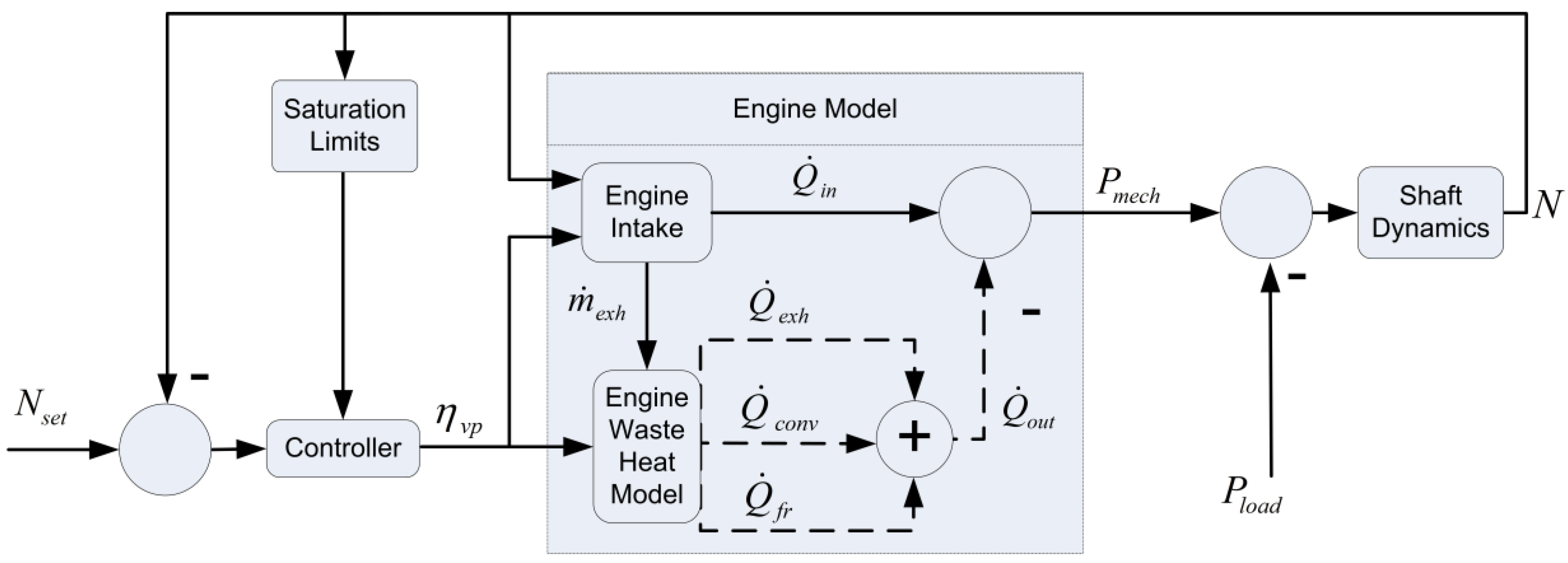
Figure 2.
Block diagram of the power component calculator subsystem.
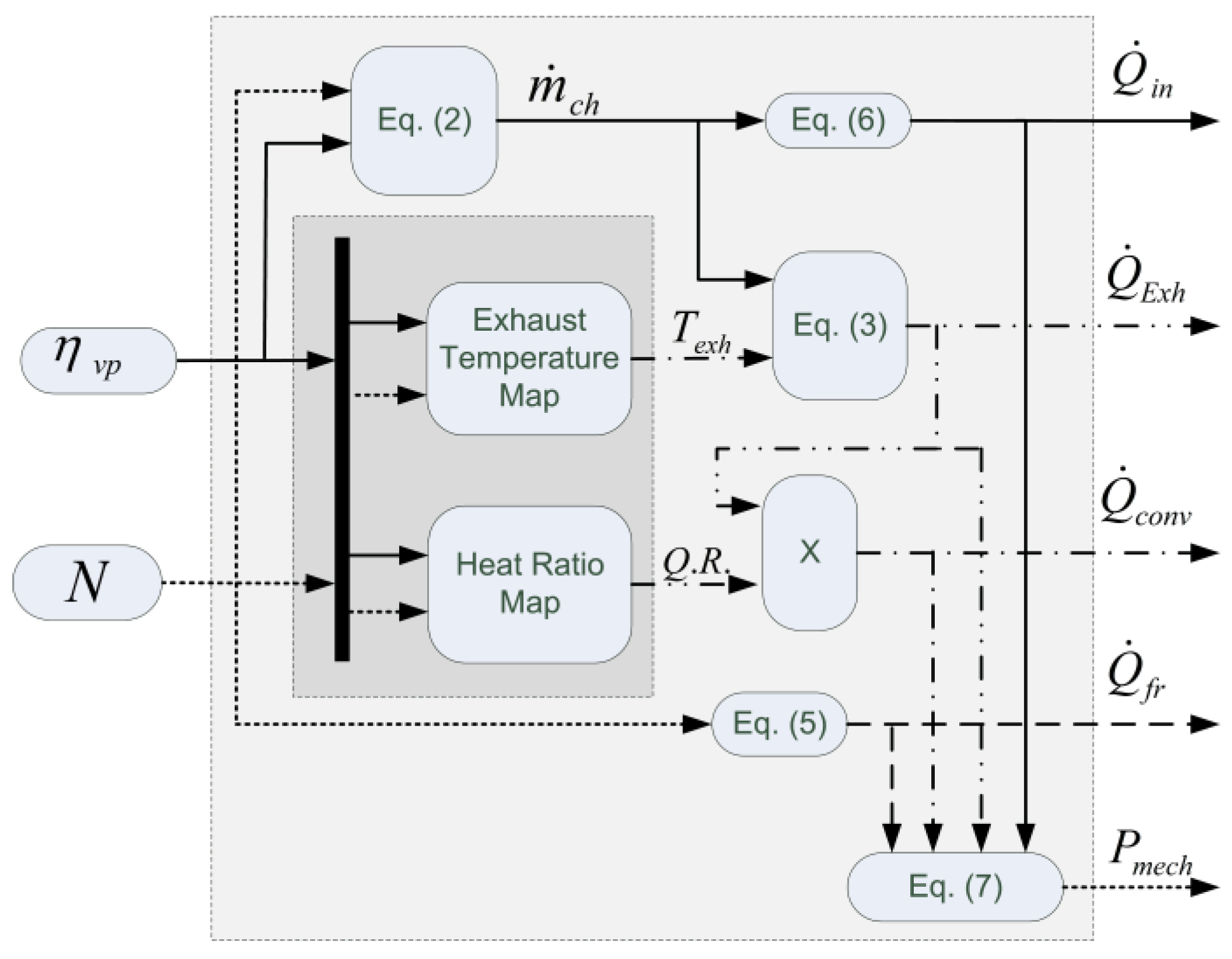
Figure 3.
Map of the exhaust temperature vs. engine speed and volumetric efficiency.

Figure 4.
Map of calculated Heat Ratio Q.R. vs. engine speed and volumetric efficiency.
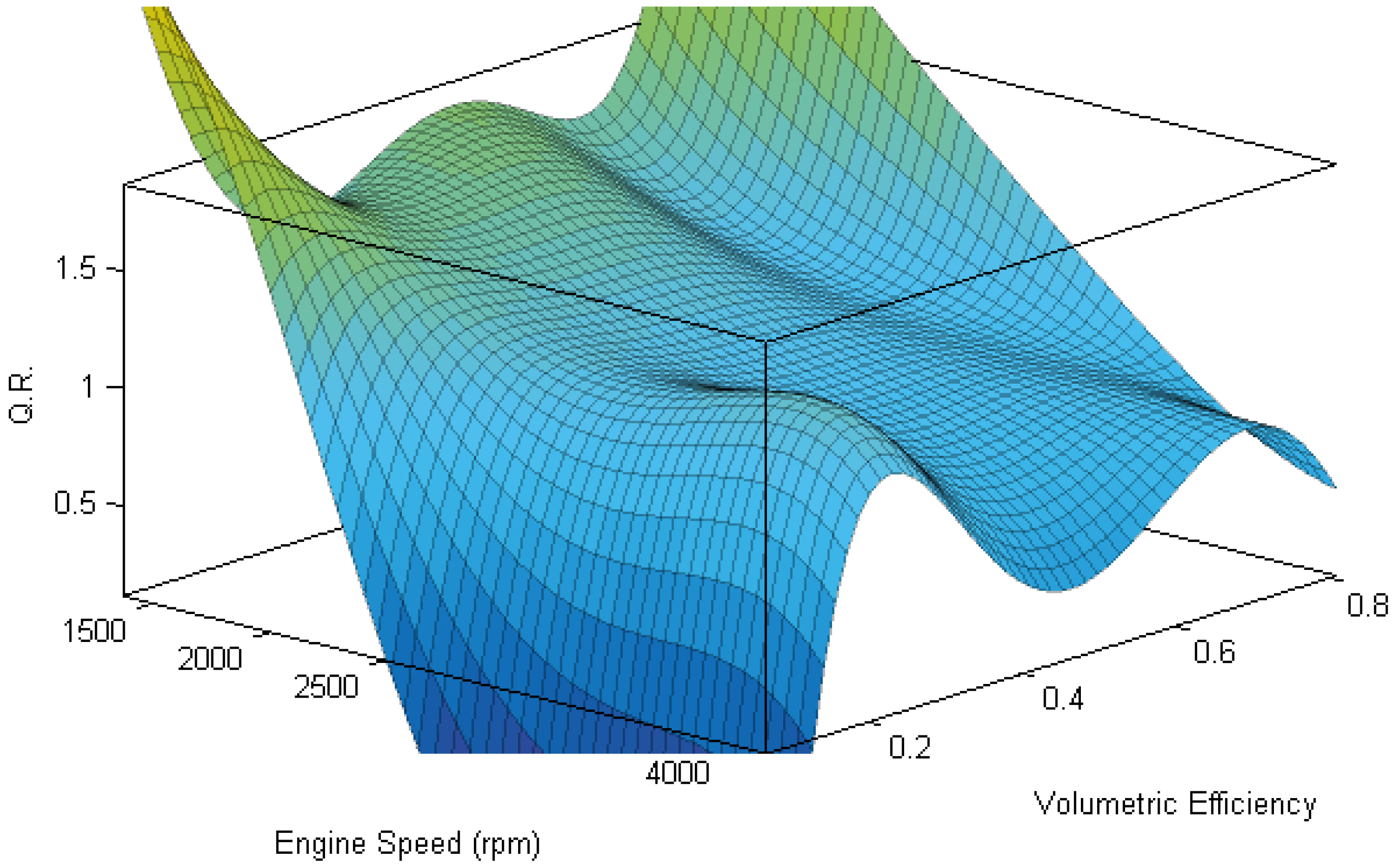
Figure 5.
Block diagram of the use of the engine model with a simple exhaust heat recovery system.

Figure 6.
Simulated power component distribution vs. time as predicted by the engine model.

Figure 7.
Simulated system electrical load and engine exhaust temperature plotted against time.

Figure 8.
Plot of combined heat and power (CHP) Electrical Load and Exhaust Heat recovery efficiency curves vs. time.
Figure 8.
Plot of combined heat and power (CHP) Electrical Load and Exhaust Heat recovery efficiency curves vs. time.

Figure 9.
Plots of the simulated and tested heat inlet rate as well as the electrical load vs. time.
Figure 9.
Plots of the simulated and tested heat inlet rate as well as the electrical load vs. time.

Figure 10.
Plot of the relative error of the estimated fuel input by the model vs. time.
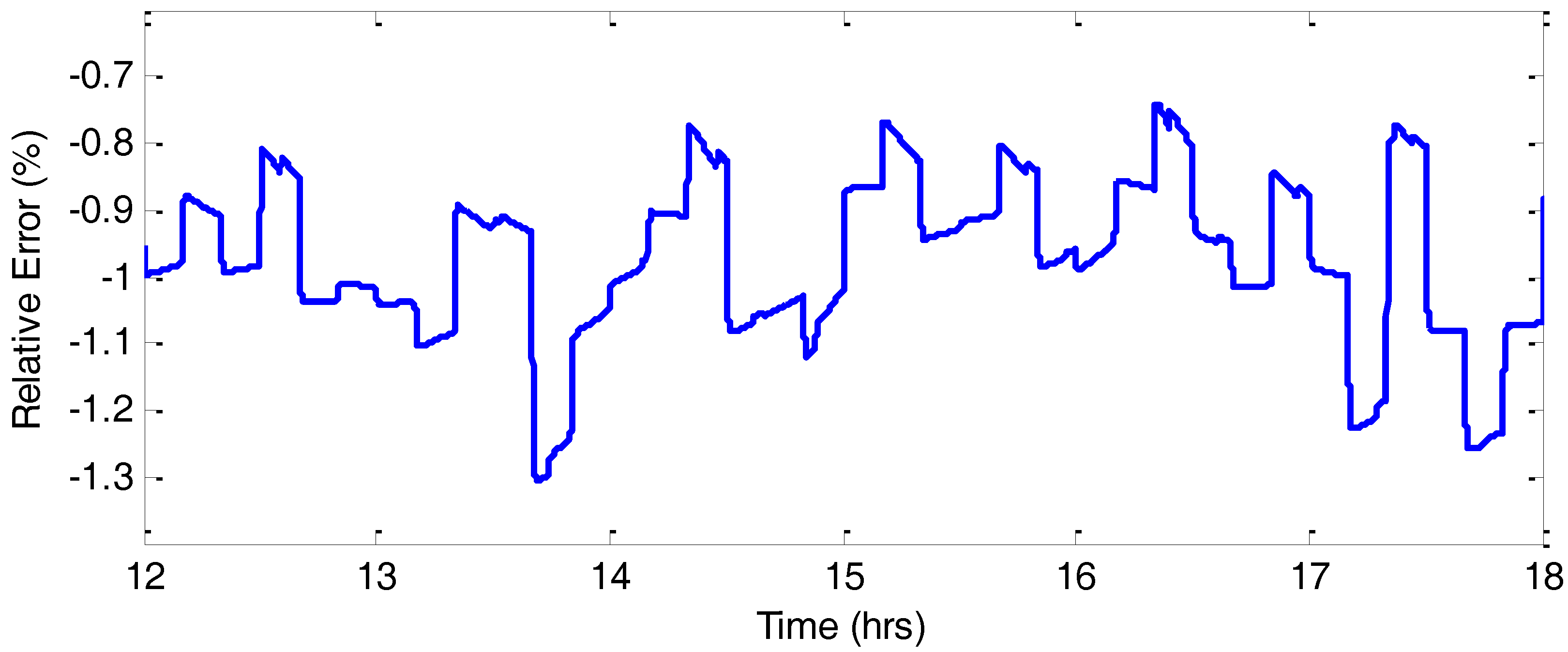
Figure 11.
Plots of the simulated and the measured exhaust temperatures vs. time.
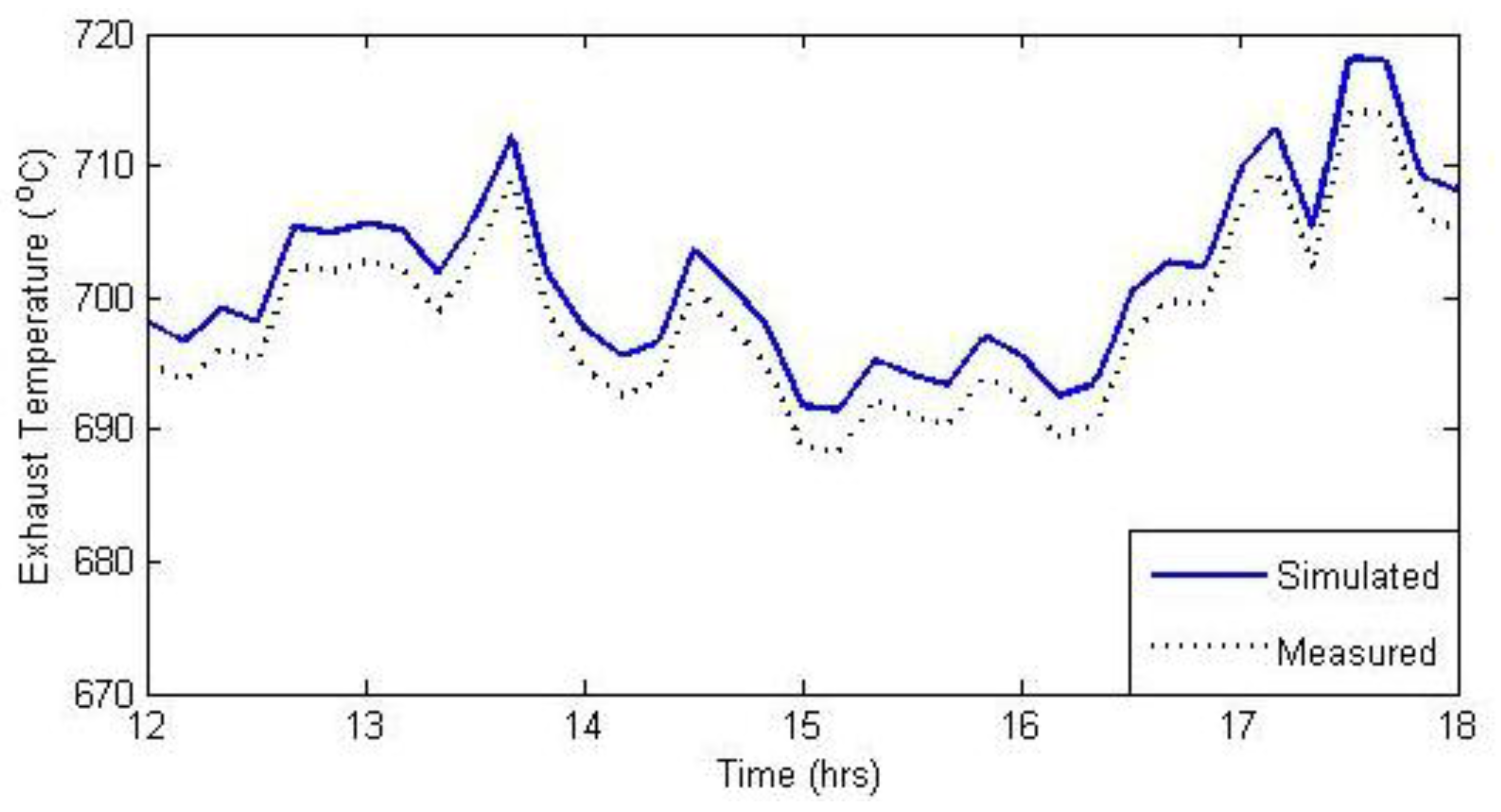
Figure 12.
Relative error of the exhaust temperature predicted by the model.

Table 1.
Characteristics and settings of the tested engine.
| Test Engine Characteristics and Settings | |
|---|---|
| Engine type | SI, Naturally Aspirated, direct injection |
| Displacement | 1.6 L |
| Number of Cylinders | 4 |
| Engine Control Unit (ECU) settings | Constant stoich. AFR, Spark at MBT |
© 2017 by the authors. Licensee MDPI, Basel, Switzerland. This article is an open access article distributed under the terms and conditions of the Creative Commons Attribution (CC BY) license (http://creativecommons.org/licenses/by/4.0/).
Share and Cite
MDPI and ACS Style
Kalantzis, N.; Pezouvanis, A.; Ebrahimi, K.M. Internal Combustion Engine Model for Combined Heat and Power (CHP) Systems Design. Energies 2017, 10, 1948. https://doi.org/10.3390/en10121948
AMA Style
Kalantzis N, Pezouvanis A, Ebrahimi KM. Internal Combustion Engine Model for Combined Heat and Power (CHP) Systems Design. Energies. 2017; 10(12):1948. https://doi.org/10.3390/en10121948
Chicago/Turabian StyleKalantzis, Nikolaos, Antonios Pezouvanis, and Kambiz M. Ebrahimi. 2017. "Internal Combustion Engine Model for Combined Heat and Power (CHP) Systems Design" Energies 10, no. 12: 1948. https://doi.org/10.3390/en10121948
Note that from the first issue of 2016, this journal uses article numbers instead of page numbers. See further details here.