A Novel Fault Early Warning Model Based on Fault Gene Table for Smart Distribution Grids


Key Laboratory of Industrial Internet of Things & Networked Control, Chongqing University of Posts and Telecommunications, Chongqing 400065, China
*
Author to whom correspondence should be addressed.
Energies 2017, 10(12), 1963; https://doi.org/10.3390/en10121963
Submission received: 10 October 2017
/
Revised: 16 November 2017
/
Accepted: 17 November 2017
/
Published: 24 November 2017
(This article belongs to the Section F: Electrical Engineering)
Abstract
:Since a smart distribution grid has a diversity of components and complicated topology; it is very hard to achieve fault early warning for each part. A fault early warning model for smart distribution grid combining a back propagation (BP) neural network with a gene sequence alignment algorithm is proposed. Firstly; the operational state of smart distribution grid is divided into four states; and a BP neural network is adopted to explore the operational state from the historical fault data of the smart distribution grid. This obtains the relationship between each state transition time sequence and corresponding fault, and is used to construct the fault gene table. Then; a state transition time sequence is obtained online periodically, which is matched with each gene in fault gene table by an improved Smith–Waterman algorithm. If the maximum match score exceeds the given threshold, the relevant fault will be detected early. Finally, plenty of time domain simulation is performed on the proposed fault early warning model to IEEE-14 bus. The simulation results show that the proposed model can achieve efficient early fault warning of smart distribution grids.
1. Introduction
In recent years, the smart grid has become a major concern of the international community [1,2,3,4,5,6,7]. Smart distribution grids are the main connection between the main grid and power supply to users and are important parts of the smart grid [8]. Whether its operational state is normal or not directly affects the power supply to thousands of users. Meanwhile, with the access of distributed generation, the popularization of electric vehicles, and the increase of user interaction, the dynamic behavior of smart distribution grid becomes complicated, and the operational risk increases greatly [9]. In the event of power outage, there will be a great influence on social life and economic losses [10,11]. With the help of condition monitoring and fault early warning techniques, predictive maintenance and condition-based maintenance have become increasingly adopted [12]. Therefore, it is necessary to carry out more in-depth research on the condition monitoring and the fault early warning of the smart distribution grid so as to provide guidance and help for relevant management staff to predictive maintenance of smart distribution grids.
At present, many domestic and foreign scholars have put forward various solutions for the fault early warning of smart distribution grid from different angles. In [13], a fault early warning method suitable for the active distribution grid based on harmonic current is proposed. Firstly, a cloud model of harmonic current is designed and the entropy based on cloud model is used to measure the range of harmonic current during normal operation, so as to determine the anomaly threshold of harmonic current before and after the interconnection of intermittent energy. Then, comparison between the measured data with the harmonic anomaly threshold is used to determine whether the harmonic current is unusual or not. In [14], it is pointed out that the weather factor is one of the main reasons for the outage of distribution grids, and a fuzzy logic system to alleviate the impact of weather factors on distribution grids is put forward, which make relevant operators obtain more accurate fault prediction. In [15], the Bayesian network is adopted to mine the real historical faults of an electricity distribution company from the south of Sweden to obtain the relationship between the fault of the distribution grid and the affected components. In [16], it is pointed out that the short circuit current has become the most common and most destructive power system fault. The accurate prediction of short circuit fault and the size of the short circuit current is becoming more and more important. An artificial neural network is introduced to predict the size of the short circuit current of distribution grid. In [17], a model combined fuzzy comprehensive evaluation and a Bayesian approach is established to predict the operational state and warning of power transformer. In [18], a better coordination between dynamic lightning protection and state estimation of the smart grid is proposed to ensure reasonable dynamic actions and improve the lightning performance. In [19], a whole function and architecture of an early warning system, and its specific design scheme are put forward, which effectively improved the scientific approach and predictability of operation decision-making for power systems. In [20], a data-driven computational method has been proposed to address fault detection, identification, and location in smart grids. Firstly, two detection hidden Markov models (HMMs) are trained for fault detection to distinguish between normal and abnormal smart grid (SG) operation conditions. Then, if a fault occurs, the trained identification HMMs are used to identify different fault types. In [21], an approach to efficiently identify the most probable failure modes in static load distribution for a given power network is developed. This technique can help discover weak links which are saturated at the failure modes, thus providing predictive capability for improving the reliability of any power system. In [22], a method is proposed to utilize phasor measurement unit (PMU) data to compute the region of stability existence and operational margins. An automated process continuously monitors voltage constraints, thermal limits, and steady-state stability simultaneously. This approach can be used to improve the reliability of the transmission grid and to prevent major blackouts.
There are some particularly studies implementing hardware techniques for predictive maintenance and diagnostics which are worthy of our study and research. In [23], the design of an intelligent power switch (IPS) in high-voltage (HV)-CMOS technology with single chip integrated protection and self-diagnostic capabilities has been proposed. In [24], a method networking vibration measuring nodes with integrated signal processing has been proposed to address the problem of predictive diagnostics in three-phase high-power transformers.
In this paper, a novel model based on fault gene tables is proposed to achieve fault early warning for smart distribution grids. The smart distribution grid as a dynamic balance system analogous to a biological system. In analogy to the human gene bank, which aims to identify and map all human genes [25], the fault gene table is constructed to show the fault information of smart distribution grids, and then the improved Smith–Waterman is adopted to realize the fault early warning for smart distribution grids so as to provide the monitoring of system operational state for power operation and management unit scientifically and effectively based on the constructed fault gene table.
2. Design of the Fault Gene Table
The fault of smart distribution grids has a certain mapping relationship with the operation data before the fault, therefore operation data can be represented as the gene of fault. In analogy to the human gene composed of four canonical bases, the operational state of smart distribution grid can be divided into four states: excellent, good, middle and bad. Then the BP neural network evaluation model is adopted to transform the operation data of the smart distribution grid into an ordered state transition time series, namely a gene. In addition, the inputs of the BP neural network are the state goal of each bus of smart distribution grid. Thus, the mapping relationship between each state transition time series and related fault can be obtain from historical fault data sources of smart distribution grids so as to construct the fault gene table.
2.1. State Division of Smart Distribution Grids
The state division of a distribution grid is hard to have a unified standard, and many studies have different points of view. In [26], it is divided into six kinds of state: fault, early warning, over-threshold, incomplete operation, safety and optimal. In [27], it is divided into six states: normal, early warning, threshold, emergency and recovery.
In this paper, in analogy to the human gene composed of the four canonical bases, the operational state of a smart distribution grid can be divided into four states: excellent, good, middle and bad labeled as E, G, M and B, which are shown as Table 1.
2.2. Operational State Evaluation of Each Bus
The operational state goal of each bus is determined by its voltage, active power and reactive power, as shown in Equation (1).
In which, as the operational state goal of each bus ranges from 0 to 1, which is better closer to 1, otherwise is worse. is the weight of voltage, is the voltage goal of each bus, is the weight of active power, is the active power of each bus, is the weight of reactive power, and is the reactive power of each bus.
The voltage goal can be calculated as Equation (2).
where . is the present value of voltage, is the average voltage of the related bus in the historical data set, is the maximum voltage of the related bus in the historical data set, and is the minimum voltage of the related bus in the historical data set.
The active power goal can be calculated as Equation (3).
where is the present value of active power, is the average active power of the related bus in the historical data set, is the maximum active power of the related bus in the historical data set, and is the minimum active power of the related bus in the historical data set.
The reactive power goal can be calculated as Equation (4).
where is the present reactive power, is the average reactive power of the related bus in the historical data set, is the maximum reactive power of the related bus in the historical data set, and is the minimum reactive power of the related bus in the historical data set.
2.3. Operational State Evaluation Model of Smart Distribution Grid
In order to dynamically evaluate the current operational state of the smart distribution grid, it is necessary to have a comprehensive grasp of the operational condition of the smart distribution grid. Therefore, a state evaluation model based on BP neural network is proposed, which obtains the operational state by comprehensively taking each bus state into account. BP neural network has good features of fault tolerance and strong adaptive learning ability, which can improves the fault tolerance and the accuracy rate of evaluation.
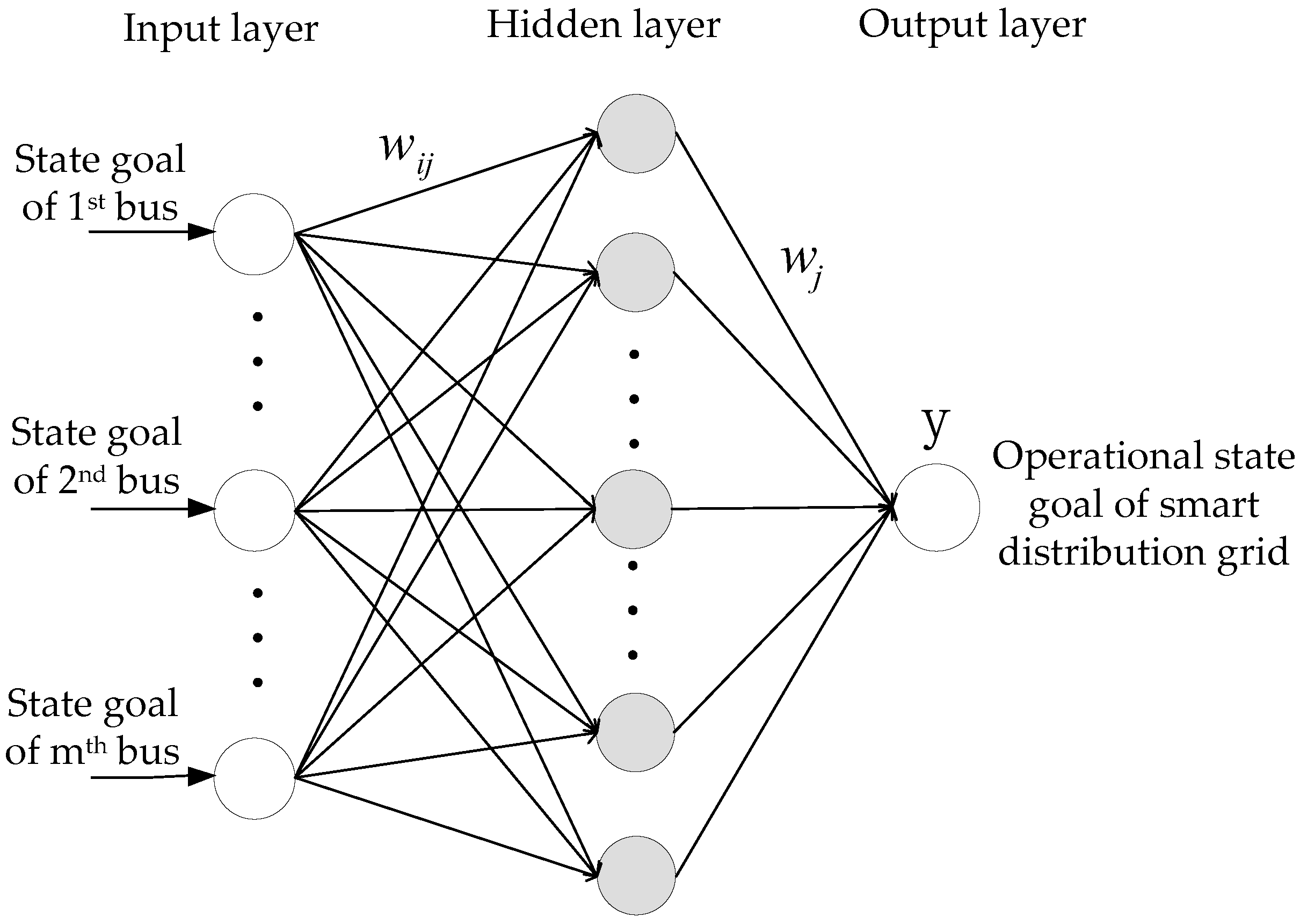
BP neural network is composed of an input layer, hidden layer and output layer. The input layer is the state goal of each bus. The output layer is the operational state of smart distribution grid. The model of BP neural network is shown as Figure 1.
The output result is divided into 4 states, which is shown as Table 2.
2.4. Fault Gene Table Construction Procedure of Smart Distribution Grid
- A k-means clustering is adopted to cluster all buses state goals of the smart distribution grid in historical fault data source into four classes, labeled with related tags including of E, G, M and B according to the magnitude of average state goal calculated by Equation (5).where denotes to different class, m is the number of buses, represents the number of groups in class, and represents the state goal of smart distribution grid in the mth bus of the zth group.
- One part of the clustered data is regarded as the training sample matrix shown as Equation (6).where n is the number of training samples, and state goal in the mth bus of the nth training sample.
- The other part of the clustered data is regarded as evaluation matrix , which is shown as Equation (7).where n∗ is the number of evaluation samples, and represents state goal in the mth bus of the evaluation sample.The training sample matrix is input into the BP neural network to determine the weights and thresholds, and the training process was as follows:
- Set the weight and threshold between input layer and hidden layer are respectively and , the weight and threshold between hidden layer and output layer are respectively and , the number of nodes in hidden layer is N, learning rate is , and the expected output of state goal is which is chosen distinct value according to the type of input sample Specifically, the for Bad(B) can be a reasonable value between 0 and 0.25, the for Middle(M) can be a reasonable value between 0.25 and 0.5, the for Good(G) can be a reasonable value between 0.5 and 0.75, and the for Excellent(E) can be a reasonable value between 0.75 and 1. For example, these expected outputs of state goals can take the mean value of the range, namely 0.125, 0.375, 0.625 and 0.875 respectively.
- Choose sigmoid function as the activation function of hidden layer and output layer, namely and , which is shown as Equation (8).
- Calculate the input and output value of each hidden neuron, which is shown as Equation (9)where is the input value of each hidden neuron, is the output value of each hidden neuron, , which denotes the index of training sample, and state goal in the ith bus of the rth training sample.
- Calculate the output value y according to the output of hidden layer , weight and threshold between hidden layer and output layer and , which is shown as Equation (10).
- Calculate the output error according to Equation (11).
- Calculate the generalization error of output layer by Equation (12).
- Calculate the generalization error of hidden layer by Equation (13).
- Adjust the weight and threshold between hidden layer and output layer and , which is calculated as Equation (14).where and are the weight and threshold between hidden layer and output layer after adjustment.
- Adjust the weight and threshold between input layer and hidden layer and , which is calculated as Equation (15).where and are the weight and threshold between input layer and hidden layer after adjustment.
- When is changed from 1 to n, all training sample is trained completely, the global error will be calculated by adding all errors of each training sample. If reaches into the specified error range, return to the step k, otherwise, set the to zero and return to step c to repeat the training.
- End the training and record the weights and thresholds of current network.
- Input the evaluation matrix into the trained BP neural network to get the state goal of the smart grid at each moment, and then compare it with the expected state to verify the effectiveness of the model. The trained BP neural network will be used to build the mapping relationship between state transition time sequence and fault so as to construct the fault gene table. The construction flow chart of fault gene table for the smart distribution grid is shown as Figure 2. The constructed fault gene table is shown as Figure 3.
3. Fault Early Warning by Improved Smith–Waterman
After the fault gene table is constructed, operation data of all buses in a smart distribution grid is obtained periodically, which is transformed into gene by BP neural network. Then, a sequence alignment algorithm is adopted to get the match score between this gene and genes in fault gene table. If the match score exceeds the given threshold, the related fault will be warned early. If the length of gene to be matched is increasing gradually, and the lengths of genes in the fault gene table are also different, it is better to use a local sequence alignment. In addition, fault early warning has a higher request of the sensitivity. Therefore, the Smith–Waterman algorithm is chosen to achieve the fault early warning of smart distribution grids, and some corresponding improvements are made to adapt to the characteristics of smart distribution grids.
3.1. Improved Smith–Waterman
Smith–Waterman algorithm aligns two sequences by matches or mismatches (also known as substitutions), insertions and deletions. Both insertions and deletions are operations that introduce gaps, which are represented by dashes. The Smith–Waterman algorithm based on the dynamic programing technique provides high sensitivity [28,29]. The procedure consists of three steps:
- Fill in the dynamic programming matrix.
- Find the maximal score in the matrix.
- Trace back the path that leads to the maximal score to find the optimal local alignment.
When the Smith–Waterman algorithm is used in biological gene sequence alignment, the importance of the four bases are the same, so the score matrix for the same base matching score is the same. In its application in the field of smart distribution grids, the analogous four bases are necessary to be different because the operational state of smart distribution grid is divided into four types with distinct performance, namely E, G, M and B.
In order to apply the request of online fault early warning of smart distribution grids, it is necessary to have some improvements to the traditional Smith–Waterman algorithm, specifically, in the design of the substitution matrix, which has two rules to be followed:
- If two states are matched, the worse the performances of two states are, the higher the match score is; namely, the match score of E with E, G with G, M with M and B with B follow an ascending order.
- If two states are mismatched, the bigger the difference between the two states is, the lower the match score. For instance, the match score of E with G, E with M and E with B follows a descending order.
The first rule can make the match between lower operational states more important, which can improve the accuracy rate of fault early warning. The second rule can lower the negative effects on fault early warning when the alignment of two states are mismatched.
According to the importance degree of each operational state and the design rules, the substitution matrix can be designed as the Equation (16).
where is the importance degree of operational state, is the state of element in the gene sequence S to be mentioned in the following paper, and is the state of element in the gene sequence U also to be mentioned in the following paper.
3.2. Procedure of Fault Early Warning by Improved Simth–Waterman
- The operation data of a smart distribution grid is obtained periodically in real time, and transformed to state transition time sequence, namely gene to be matched, by the BP neural network. The length of it gradually increases with the passage of time.
- The gene to be matched and the gene in fault gene table are matched periodically by the improved Smith–Waterman algorithm, and the matching process is as follows:
- Let gene to be matched , gene in fault gene table , and the lengths of them be and , respectively.
- Determine the substitution matrix and the gap penalty scheme.
- Construct a scoring matrix D and initialize its first row and first column. The size of the scoring matrix is (.
- Fill the scoring matrix using the Equations (17) and (18).In which, , , can be calculated by Equation (16), and are the gap penalty when the or the is dash.
- Find and to makewhere is the highest score in the scoring matrix D.
- Until all alignments are finished between genes to be matched and all genes in the fault gene table, all highest scores are obtained.
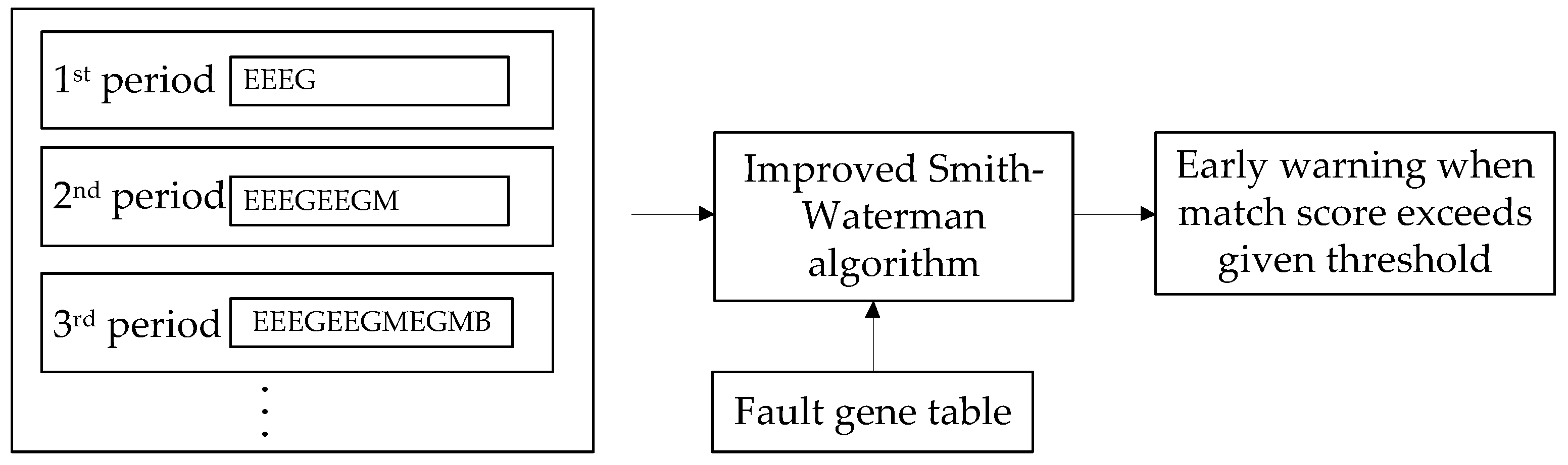
- Find the maximum score from all the highest scores, and compare it to the given threshold. If the maximum score exceeds the threshold, the related fault will be warned early. The block diagram of fault early warning for smart distribution grid realized by the improved Smith–Waterman algorithm is shown as Figure 4.
In the process of gene sequence alignment, it is very critical to set an appropriate early warning threshold. In this paper, the early warning threshold is set to the percentage of full score of fault genes in the fault gene table. Therefore, the match score of early warning is different, which depends on the length of genes in the fault gene table for better adaptability. In the following simulation, the most suitable threshold, which can make the proposed model obtain an optimal accuracy rate of fault early warning, is chosen from different early warning thresholds.
4. Simulation and Analysis
PSAT (power system analysis toolbox) based on MATLAB is adopted to do time domain simulation tests for the proposed model. The IEEE-14 bus is used as the simulation object, and random disturbance is introduced during the process of the simulation. The disturbances are randomly introduced into one of the four components including of the constant power (PQ) load, automatic voltage regulator (AVR), transmission line and synchronous machine of IEEE-14 Bus.
4.1. Simulation Parameters
The corresponding simulation parameters include the simulation parameters of the proposed model and IEEE-14 bus.
4.2. Procedure of Simulation
In the process of simulation, the random disturbances are introduced into each model of IEEE-14 bus so as to simulate the actual operating environment of the distribution grid and shorten the appearance time of faults. The simulation process is divided into two steps including the simulation of fault gene table construction and the simulation of fault early warning of smart distribution grid based on the obtained fault gene table.
4.2.1. Simulation of Fault Gene Table Construction
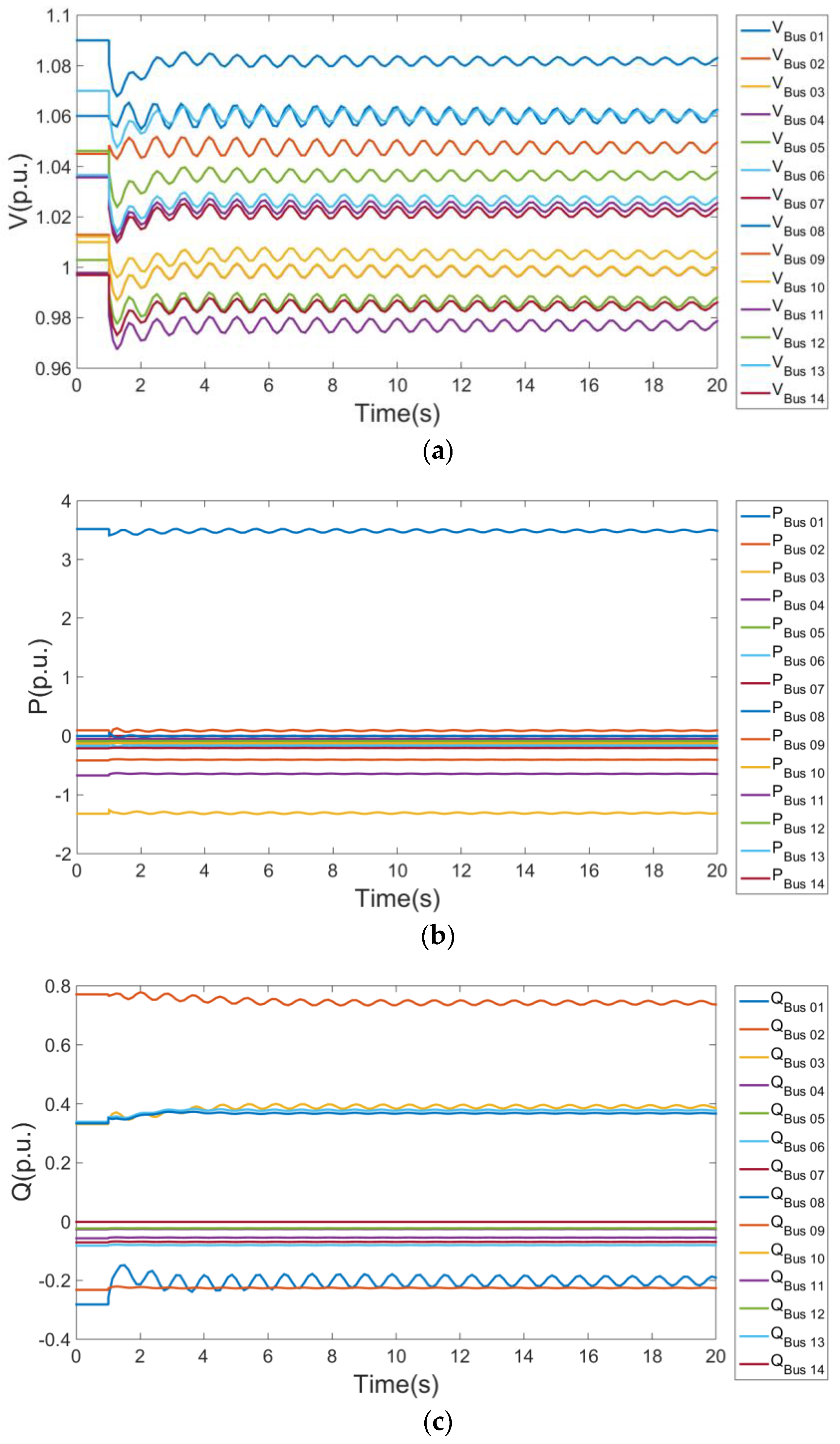
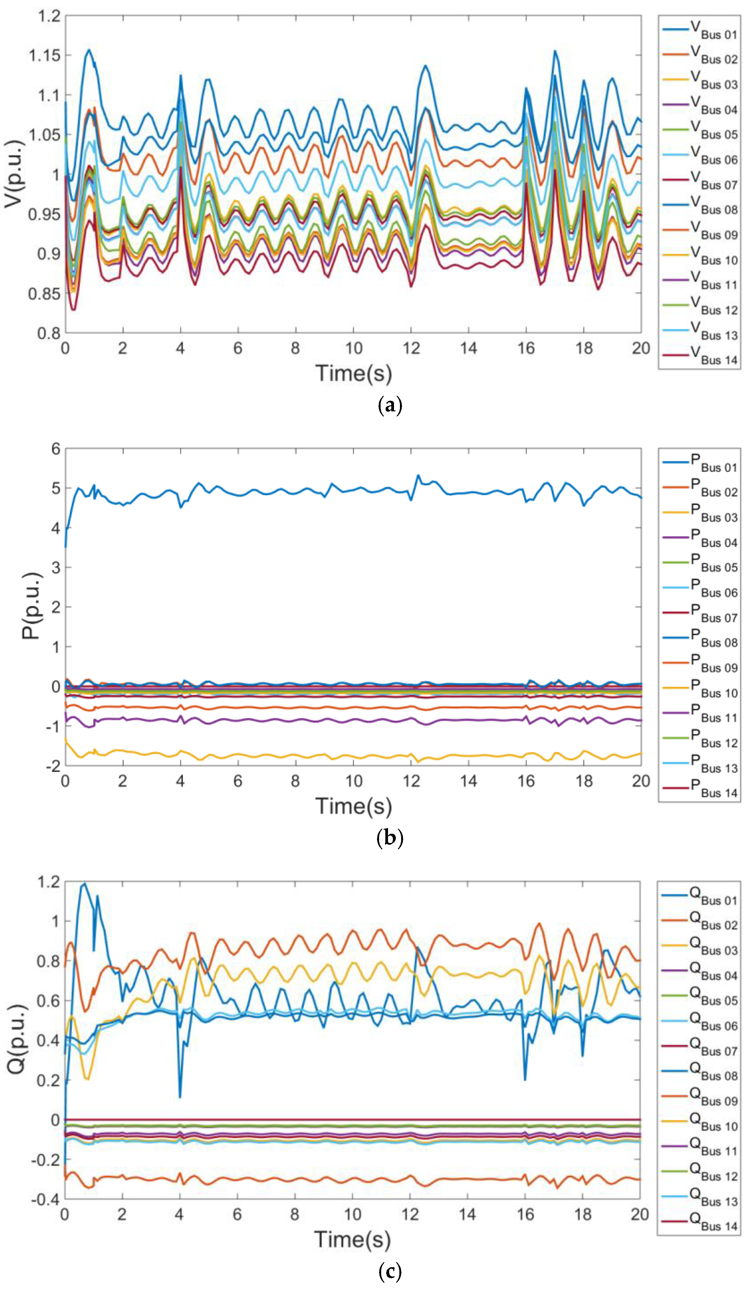
Firstly, PSAT based on MATLAB is adopted to do time domain simulation on the IEEE-14 bus. The simulation time is 20 s. Two types of operation data of each bus are obtained. One type is the normal operation data of each bus about voltage, active power and reactive power of distribution grid without any disturbance, which is shown as Figure 6. The other is the operation data with random disturbances per second during the simulation, which is shown as Figure 7.
In Figure 6a–c, the change of the three parameters of each bus are very regular, namely the state fluctuation of each bus is very regular without any disturbance. In Figure 7a–c, the fluctuation of voltage and reactive power in each bus is strong, while the fluctuation of active power in each bus is weak.
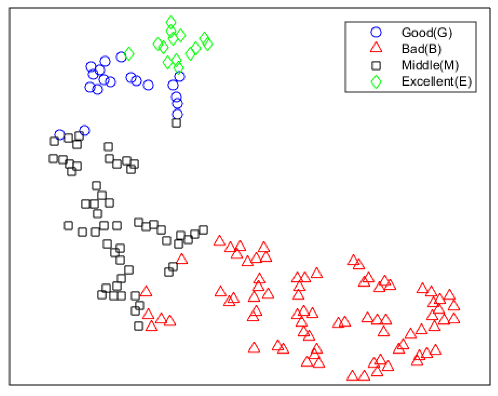
Simulation data about three parameters of each bus to first fault is exported by PSAT, and 166 groups of voltage, active power and reactive power are obtained, respectively. The comprehensive operational state goal of each bus can be calculated by Equations (1)–(4) with the simulation data. Then, a k-means clustering is adopted to cluster the data about state goal of each bus into four classes, labeled with related tags including of E, G, M and B according to the magnitude of average state goal calculated by Equation (5). The clustered data is a high-dimensional dataset for the number of buses is 14. A dimensionality reduction algorithm named t-Distributed Stochastic Neighbor Embedding (t-SNE) [30,31] is adopted to model the high-dimensional data by a two-dimensional point, which then is visualized in a scatter plot shown as Figure 8.
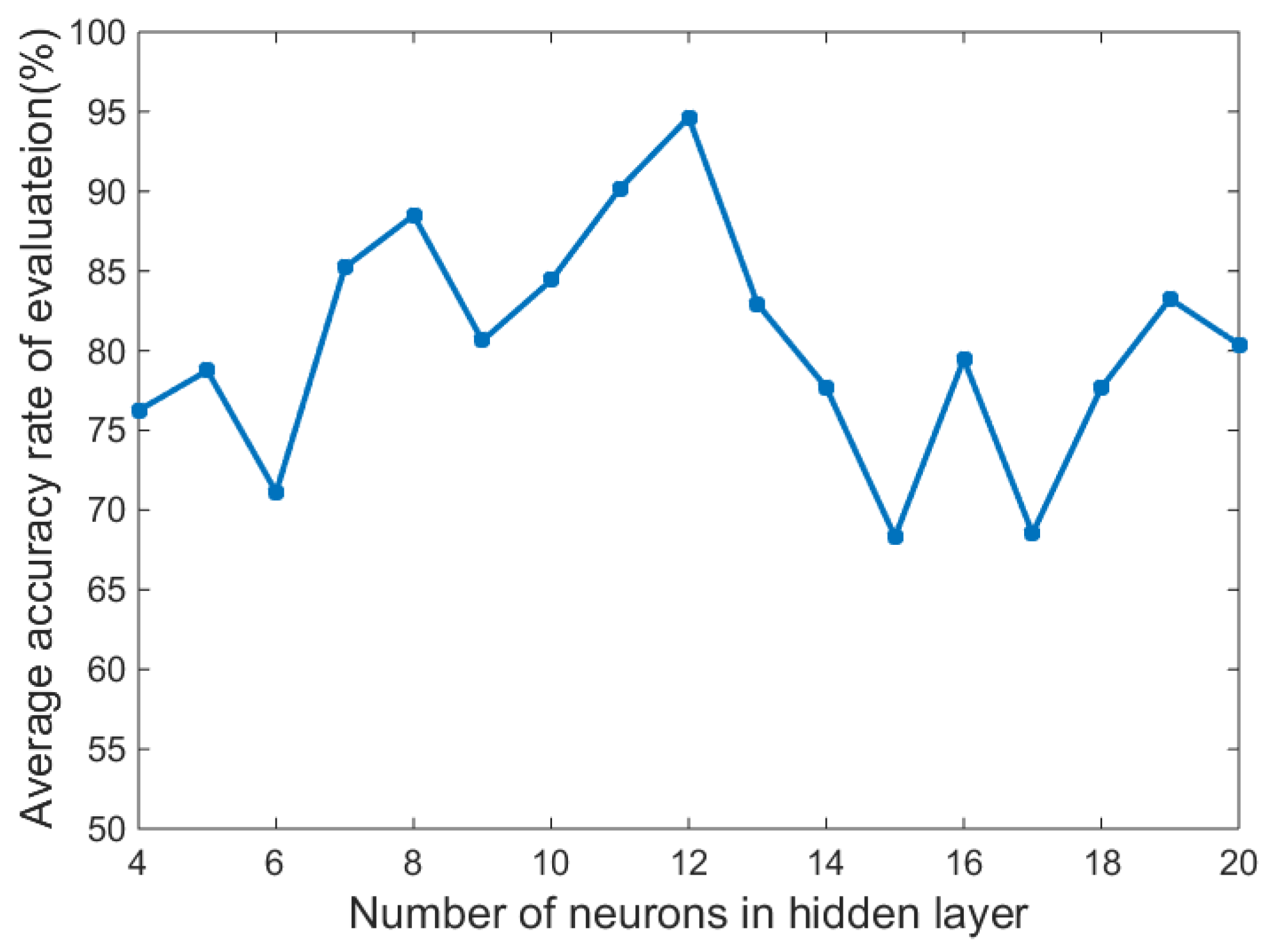
A 10-fold cross-validation is adopted on the obtained 166 groups of data to get the relation between the average accuracy rate of BP neural network evaluation model and the number of neurons in hidden layer. As the number of neurons in hidden layer ranges from 4 to 20, the relation between them is shown as Figure 9.
In Figure 9, the BP neural network evaluation model has the highest average accuracy rate close to 95%, when the number of neurons in a hidden layer is 12.
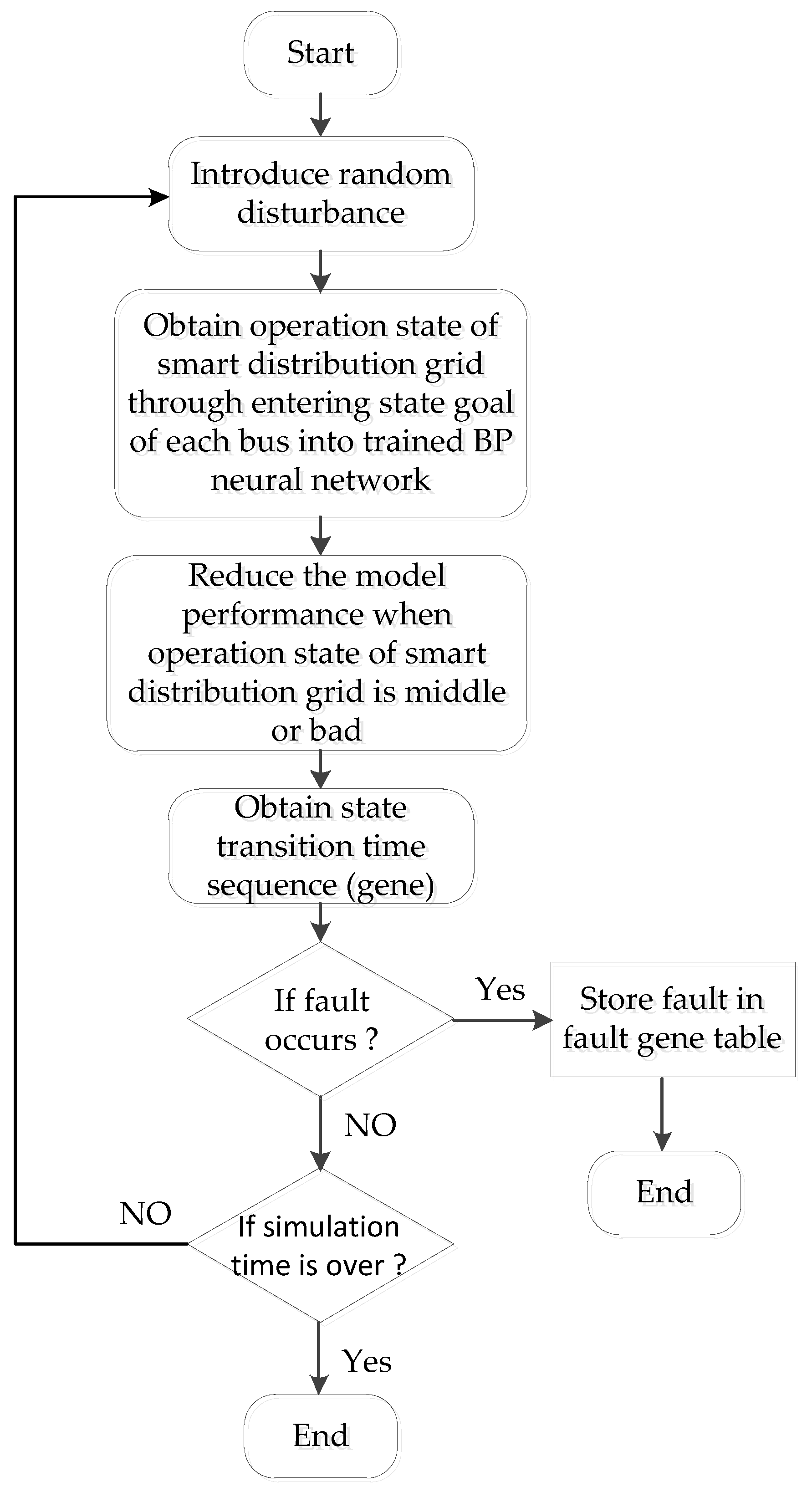
After the BP neural network state evaluation model is trained and the number of neurons in the hidden layer is set to 12, the goal of each bus in each time domain simulation with random disturbances is firstly transformed into a data sequence with a sampling period of 0.5 s, and then this data sequence is input into the trained BP neural network evaluation model to obtain a state transition time sequence and its related fault. In each time domain simulation, the flow diagram of the fault gene table construction is shown in Figure 10.
According to Figure 10, plenty of time domain simulations with random disturbances are made, and the relationship between the fault and the state transition time sequence is obtained in each time domain simulation, which is used to construct the fault gene table. The faults in the fault gene table are mainly composed of four component faults shown in Table 8.
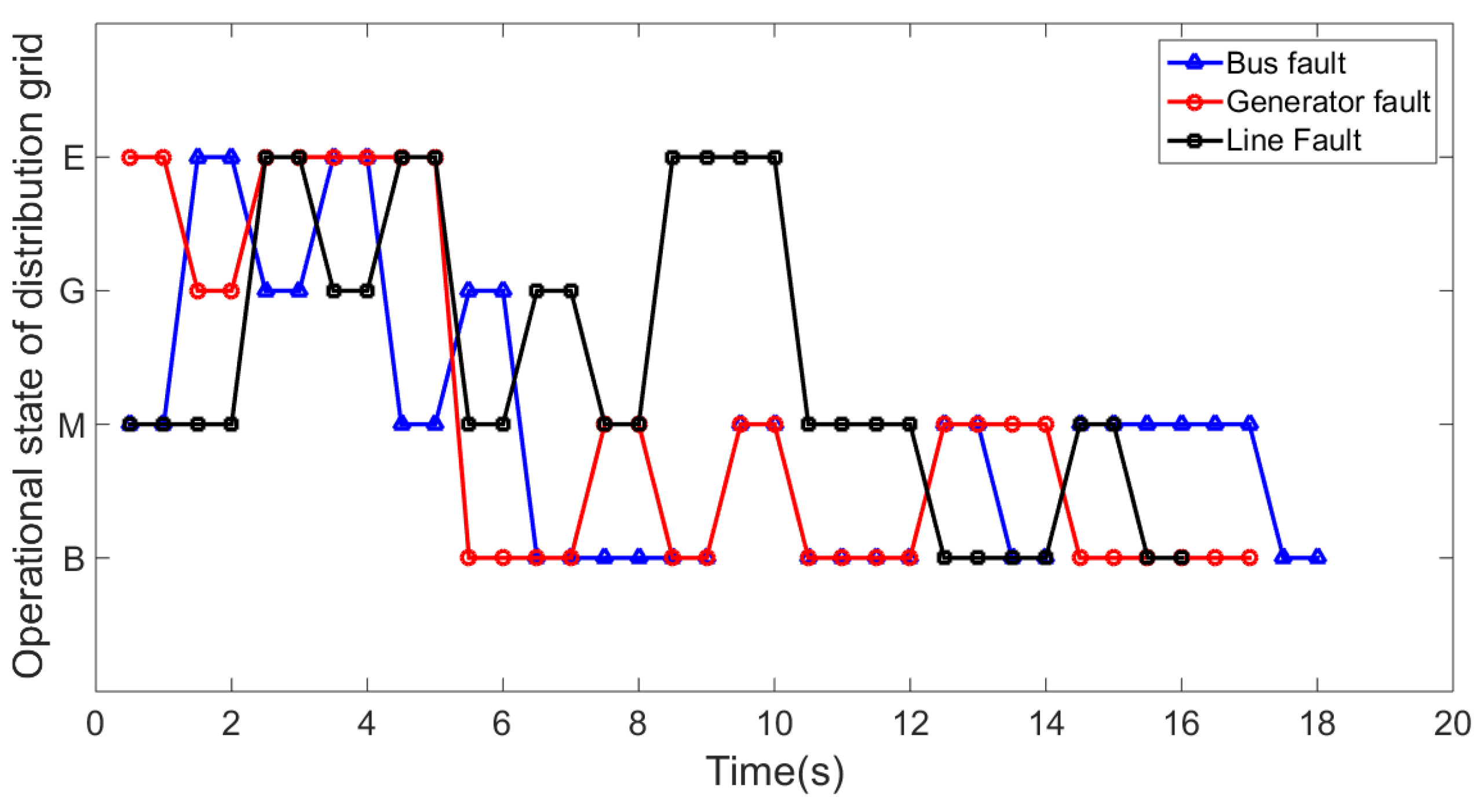
Three typical relationships between sate transition time sequences and related component faults are given in Figure 11.
In Figure 11, it can be concluded that smart distribution grid has been in a lower operation before the occurrence of a fault.
4.2.2. Simulation of Fault Early Warning
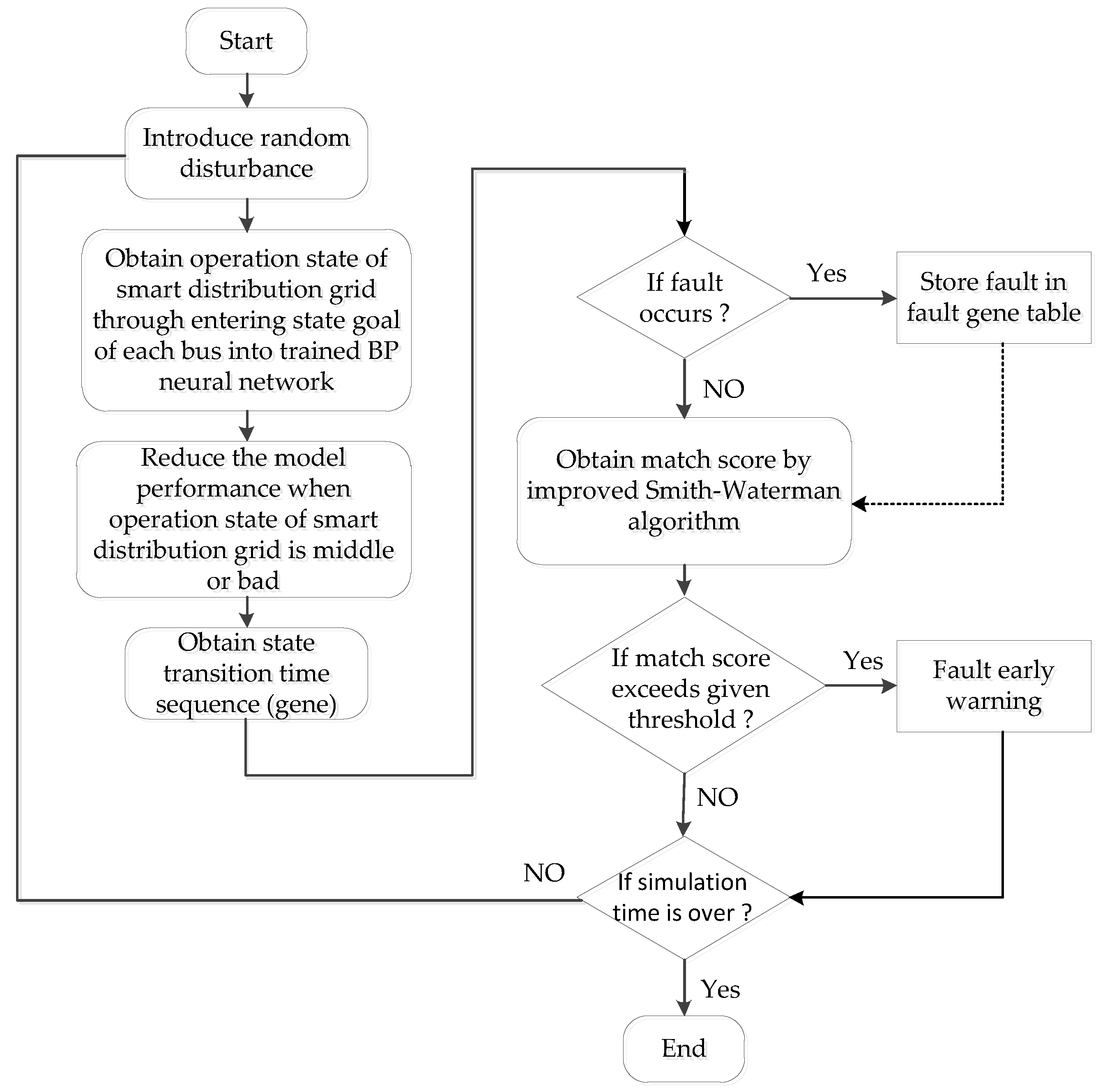
PSAT based on MATLAB is adopted to do time domain simulation added with random disturbances on IEEE-14 bus with a simulation time of 20 s. During the time domain simulation, state transition time sequence as a gene is obtained periodically, which is used to match with the genes in the fault gene table by the improved Smith–Waterman algorithm. If the match score exceeds the given threshold, the related fault will be warned early. The flow diagram of fault early warning is shown in Figure 12.
According to Equation (16) and Table 6, the substitution matrix for gene sequence alignment is shown in Table 9.
If a fault occurs during a time domain simulation, and the proposed model fails to give the fault, or the gene related to the fault is a new type, then it is necessary to be stored in the fault gene table for improving the accuracy rate of fault early waning in the following simulation. The total number of proposed models giving a right fault early warning and occurring faults are recoded respectively, and then the accuracy rate of fault early warning is calculated by the Equation (20).
where T is the number of giving a right fault early warning, C is the total number of occurring faults, and is the accuracy rate of fault early warning.
If the threshold and weights of three parameters in each bus are different, the accuracy rate of fault early warning is different. In order to know the relation between them, four sets of different weights are chosen and threshold ranges from 0.6 to 0.9. The relations between the average accuracy rate of fault early warning and threshold in different weights are obtained using plenty of simulations as shown in Figure 13.
In Figure 13, the following can be concluded:
- In terms of weights: the accuracy rate of fault early warning is higher when the weights of voltage and reactive power of each bus is bigger. The threshold has a trend of decreasing at the maximum accuracy rate of fault early warning with the decrease of voltage weight.
- In terms of threshold: when the threshold is too small, the probability of error is higher due to the interference of the other similar fault genes. While the threshold is too large, the probability of that fault occurring before the match score reaches the threshold is higher.
Therefore, when selecting the weights of the parameters of the bus, it is better to choose slightly higher weights of voltage and reactive power in each bus, and slightly lower weights of active power. As to threshold, it is not necessary to select too large or too small thresholds, and an appropriate threshold is better. In Figure 13, when , and the threshold is chosen as 0.8, the proposed model has the highest average accuracy rate of fault early warning by 94%.
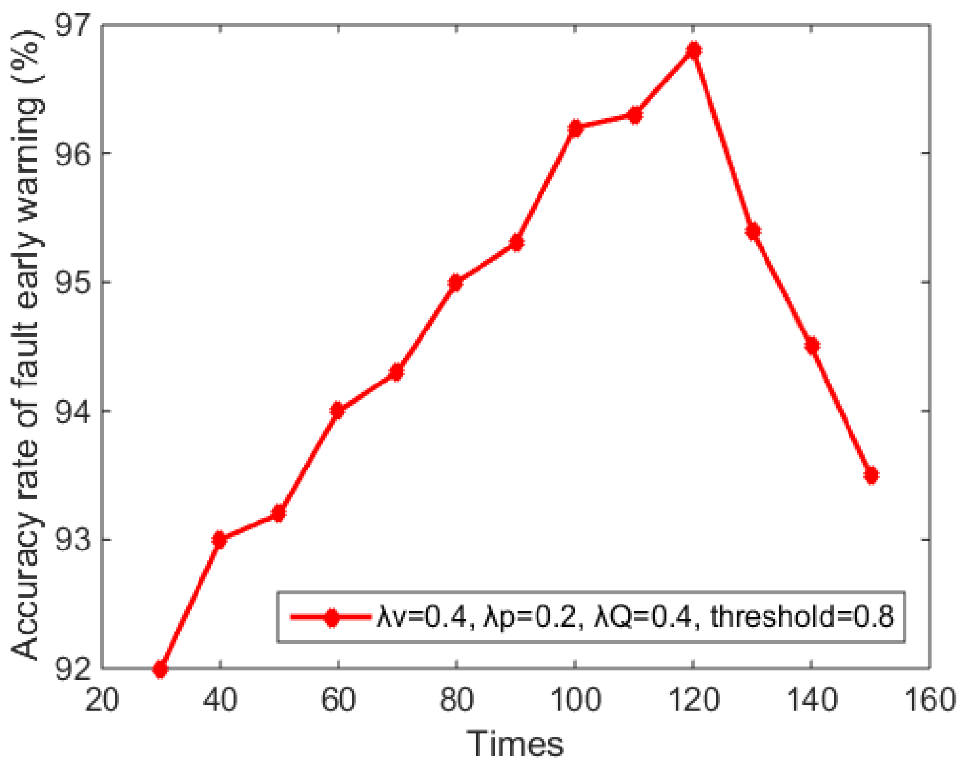
With the times of simulation increasing, the fault genes failed to warn early. This will be added into the fault gene table, which can increase the accuracy rate of fault early warning later. In order to know the relation between the accuracy rate and times of simulation, the current best weights and threshold are chosen as , threshold = 0.8, and the accuracy rate changes with the times ranges from 30 to 150 as shown in Figure 14.
In Figure 14, the change trend of accuracy rate can be divided into two parts. The first part shows that the accuracy rate increases with the times of simulation because the fault genes which failed to warn early are added into the fault gene table. The second part denotes that the accuracy rate decreases with the times of simulation because the number of fault genes in the fault gene table is too large, which causes redundancies and introduces disturbances. Therefore, the accuracy rate of fault early warning has a tendency to converge to one at the beginning. When the times reach 120, the accuracy rate of fault early warning is close to 97%.
In the field of fault early warning for smart distribution grids, due to the difference of data source access and the difference of needed data for distinct models, it is hard to take a quantitative approach to compare the proposed model with the existing models for fault early warning. Therefore, a qualitative approach is taken to compare these models to some degrees, which is shown as Table 10.
5. Conclusions
In this paper, the proposed model combined BP neural network and the Smith–Waterman gene sequence alignment algorithm, fully exploiting fault features of smart distribution grids, which provides a new thought in the solution of fault early warning for smart distribution grids. In practice, the historical fault data source including voltage, active power and reactive power in each bus can be transformed into a fault gene table by the BP neural network, and then an improved Smith–Waterman is adopted to match the current state transition time sequence (gene) with the genes in the fault gene table. If the match score exceeds a given threshold, the related fault will be warned early. The proposed model has strong versatility and adaptability due to a different fault gene table that can be constructed when confronted with different scale and more complicated topology of a smart distribution grid. PSAT based on MATLAB is adopted to do time domain simulations of proposed models on the object of IEEE-14 bus. The simulation result shows that the proposed model can achieve the fault early warning for smart distribution grids efficiently and with a high accuracy rate with a tendency to converge to one. It provides operational monitoring and maintenance guidance of smart distribution grids for relevant managers and effectively improves the scientific characteristics and predictability of operational decision-making for power systems.
There are actually some limitations in the proposed model. It can only perform the fault early warning in the most faults of smart distribution grid which have features of tendency and cumulative effect. The transient faults caused by the improper operation or extreme weather are hard to be addressed by the proposed model.
Fault gene tables relating to different scales of smart distribution grids have certain differences, but also have a certain generality to some extent. Therefore, in further research, it can be considered that an association rule algorithm such as Apriori and FP-Growth can be used to refine the fault gene tables related to different scales of smart distribution grids so as to make fault gene tables that have better universality.
Acknowledgments
The research was supported by the Project of Science and Technology of State Corporation of China (Grant No. SGJSSZOOFZJS1501091) and the Basic and Frontier Research Project of Chongqing (Grant No. cstc2015jcyjA40007 and No. cstc2015jcyjA40009).
Author Contributions
M.X. and J.M. conceived and designed the experiments; J.M. performed the experiments; Z.W. and J.M. analyzed the data; P.G. contributed analysis tools; J.M. wrote the paper.
Conflicts of Interest
The authors declare no conflict of interest.
References
- Ardito, L.; Procaccianti, G.; Menga, G.; Morisio, M. Smart Grid Technologies in Europe: An Overview. Energies 2013, 6, 251–281. [Google Scholar] [CrossRef]
- Chu, C.C.; Lu, H.C. Complex Networks Theory for Modern Smart Grid Application: A Survey. IEEE J. Emerg. Sel. Top. Circ. Syst. 2017, 7, 177–191. [Google Scholar] [CrossRef]
- Mahdad, B.; Srairi, K. Blackout risk prevention in a smart grid based flexible optimal strategy using Grey Wolf-pattern search algorithms. Energy Convers. Manag. 2015, 98, 411–429. [Google Scholar] [CrossRef]
- Andrén, F.P.; Strasser, T.I.; Kastner, W. Engineering Smart Grids: Applying Model-Driven Development from Use Case Design to Deployment. Energies 2017, 10, 374. [Google Scholar] [CrossRef]
- Fang, X.; Misra, S.; Xue, G.; Yang, D. Smart Grid-The New and Improved Power Grid: A Survey. IEEE Commun. Surv. Tutor. 2012, 14, 944–980. [Google Scholar] [CrossRef]
- Missaoui, R.; Warkozek, G.; Bacha, S.; Ploix, S. Real Time Validation of an Optimization Building Energy Management Strategy Based on Power-Hardware-in-the-loop Tool. In Proceedings of the IEEE PES International Conference and Exhibition on Innovative Smart Grid Technologies, Berlin, Germany, 14–17 October 2012; pp. 1–7. [Google Scholar]
- Ciabattoni, L.; Comodi, G.; Ferracuti, F.; Fonti, A.; Giantomassi, A.; Longhi, S. Multi-apartment residential microgrid monitoring system based on kernel canonical variate analysis. Neurocomputing 2015, 170, 306–317. [Google Scholar] [CrossRef]
- Lu, Y.; Liu, D.; Liu, J. Information Integration Demand and Model Analysis for Smart Distribution Grid. Autom. Electr. Power Syst. 2010, 34, 1–4. [Google Scholar]
- Li, T.; Xu, B. Self-healing and its benchmarking of smart distribution grid. Power Syst. Prot. Control 2010, 38, 105–108. [Google Scholar]
- Wang, C.; Grebogi, C.; Baptista, M.S. Control and prediction for blackouts caused by frequency collapse in smart grids. Chaos 2016, 26, 22–29. [Google Scholar] [CrossRef] [PubMed]
- Jia, Y.; Xu, Z.; Lai, L.L.; Wong, K.P. Risk-based power system security analysis considering cascading outages. IEEE Trans. Ind. Inform. 2016, 12, 872–882. [Google Scholar] [CrossRef]
- Lu, B.; Li, Y.; Wu, X.; Yang, Z. A Review of Recent Advances in Wind Turbine Condition Monitoring and Fault Diagnosis. In Proceedings of the 2009 IEEE Power Electornics and Machines in Wind Applications, Lincoln, NE, USA, 24–26 June 2009; pp. 1–7. [Google Scholar]
- Zhong, Q.; Zhang, W.; YU, H.; Li, L.; Wang, L. Research on harmonic forecasting and warning of active distribution network. Power Syst. Prot. Control 2014, 42, 50–56. [Google Scholar]
- Chen, P.C.; Kezunovic, M. Fuzzy Logic Approach to Predictive Risk Analysis in Distribution Outage Management. IEEE Trans. Smart Grid 2016, 7, 2827–2836. [Google Scholar] [CrossRef]
- Nemati, H.M.; Sant’Anna, A.; Nowaczyk, S. Bayesian Network representation of meaningful patterns in electricity distribution grids. In Proceedings of the 2016 IEEE International Energy Conference (ENERGYCON), Leuven, Belgium, 4–8 April 2016; pp. 1–6. [Google Scholar]
- Li-an, C. Prediction for Magnitude of Short Circuit Current in Power Distribution System Based on ANN. In Proceedings of the 2011 International Symposium on Computer Science and Society, Kota Kinabalu, Malaysia, 16–17 July 2011; pp. 130–133. [Google Scholar]
- Shi, S.; Wang, K.; Chen, L. Power transformer status evaluation and warning based on fuzzy comprehensive evaluation and Bayes discrimination. Electr. Power Autom. Equip. 2016, 36, 60–66. [Google Scholar]
- Tong, C.; Gao, Y.; Wang, Q. Coordination of Dynamic Lightning Protection and Smart Grids State Estimation. In Proceedings of the 2014 International Conference on Lightning Protection (ICLP), Shanghai, China, 11–18 October 2014; pp. 1027–1035. [Google Scholar]
- Zhen, C.; Hou, J.; Yan, J. Functional Design and Implementation of Online Dynamic Security Assessment and Early Warning System. Power Syst. Technol. 2010, 34, 55–60. [Google Scholar]
- Jiang, H.; Zhang, J.J.; Gao, W.; Wu, Z. Fault Detection, Identification, and Location in Smart Grid Based on Data-Driven Computation Methods. IEEE Trans. Smart Grid 2014, 5, 2947–2956. [Google Scholar] [CrossRef]
- Chertkov, M.; Pan, F.; Stepanov, M.G. Predicting Failures in Power Grids: The Case of Static Overloads. IEEE Trans. Smart Grid 2010, 2, 162–172. [Google Scholar] [CrossRef]
- Vaiman, M.; Vaiman, M.; Maslennikov, S.; Litvinov, E.; Luo, X. Calculation and Visualization of Power System Stability Margin Based on PMU Measurements. In Proceedings of the First IEEE International Conference on Smart Grid Communications, Gaithersburg, MD, USA, 4–6 October 2010; pp. 31–36. [Google Scholar]
- Costantino, N.; Serventi, R.; Tinfena, F.; D’Abramo, P.; Chassard, P.; Tisserand, P.; Saponara, S.; Fanucci, L. Design and Test of an HV-CMOS Intelligent Power Switch With Integrated Protections and Self-Diagnostic for Harsh Automotive Applications. IEEE Trans. Ind. Electron. 2011, 58, 2715–2727. [Google Scholar] [CrossRef]
- Saponara, S.; Fanucci, L.; Bernardo, F.; Falciani, A. Predictive Diagnosis of High-Power Transformer Faults by Networking Vibration Measuring Nodes with Integrated Signal Processing. IEEE Trans. Instrum. Meas. 2016, 65, 1749–1760. [Google Scholar] [CrossRef]
- Conley, J.M.; Mitchell, R.; Cadigan, R.J. A Trade Secret Model for Genomic Biobanking. J. Law Med. Ethics 2012, 40, 612–629. [Google Scholar] [CrossRef] [PubMed]
- Chen, X.; Gu, X.; Xu, K. Architecture for Self-healing Control of Urban Power Grid. Autom. Electr. Power Syst. 2009, 33, 38–42. [Google Scholar]
- Jia, D.; Meng, X.; Song, X. Technology Framework of Self-Healing Control in Smart Distribution Grid. Power Syst. Clean Energy 2011, 27, 14–18. [Google Scholar]
- Huang, L.T.; Wu, C.C.; Lai, L.F.; Li, Y.J. Improving the mapping of smith-waterman sequence database searches onto CUDA-Enabled GPUs. BioMed Res. Int. 2015, 2015, 185179. [Google Scholar] [CrossRef] [PubMed]
- Okada, D.; Ino, F.; Hagihara, K. Accelerating the smith-waterman algorithm with interpair pruning and band optimization for the all-pairs comparison of base sequences. BMC Bioinform. 2015, 16, 321. [Google Scholar] [CrossRef] [PubMed]
- Laurens, V.D.M. Accelerating t-SNE using tree-based algorithms. J. Mach. Learn. Res. 2014, 15, 3221–3245. [Google Scholar]
- Laurens, V.D.M.; Hinton, G.; Hinton, V.D.M.G. Visualizing Data using t-SNE. J. Mach. Learn. Res. 2008, 9, 2579–2605. [Google Scholar]
Figure 1.
Model of three-layer back propagation (BP) neural network.

Figure 2.
Fault gene table construction of smart distribution grid.
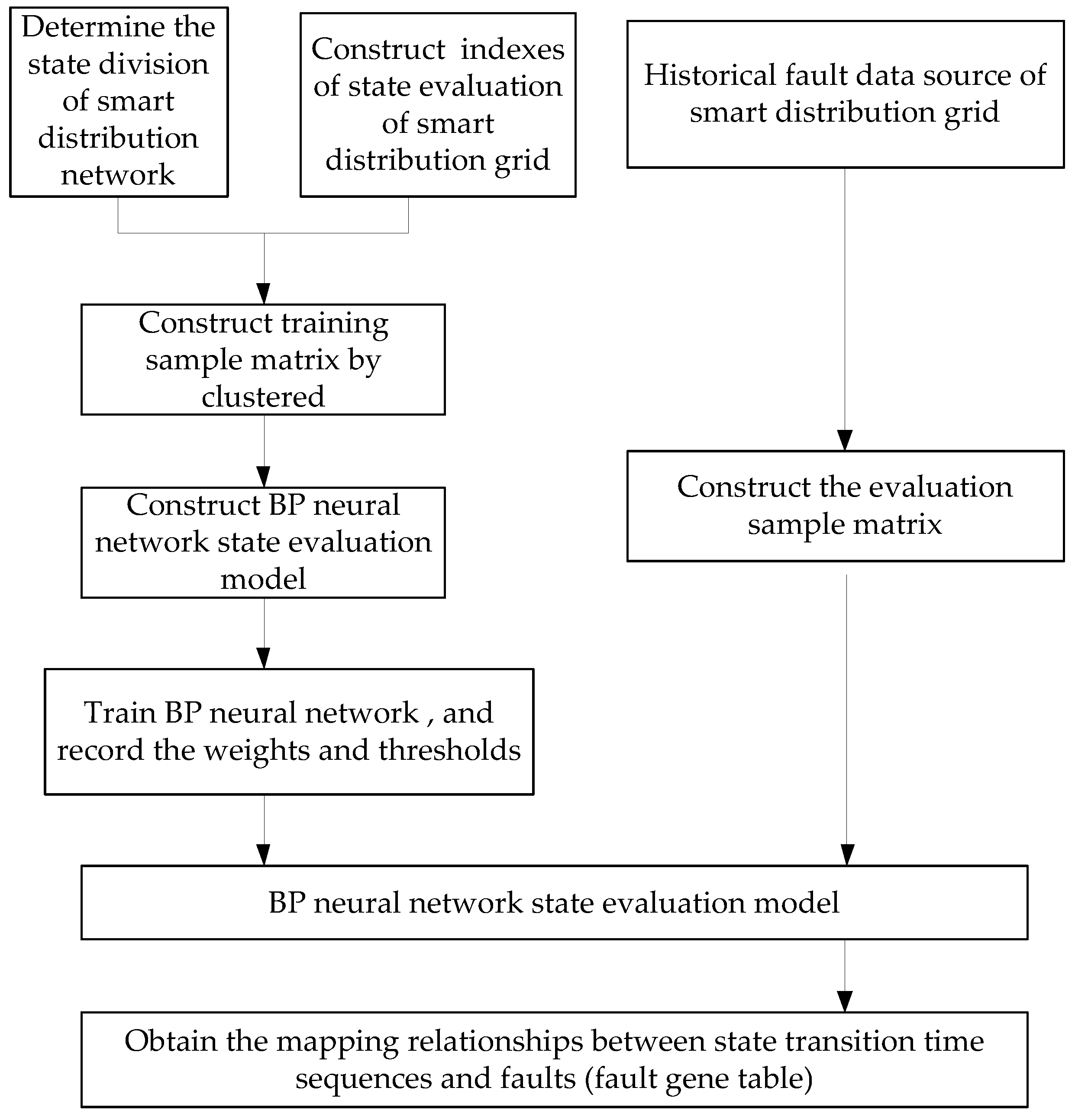
Figure 3.
Fault gene table of smart distribution grid.
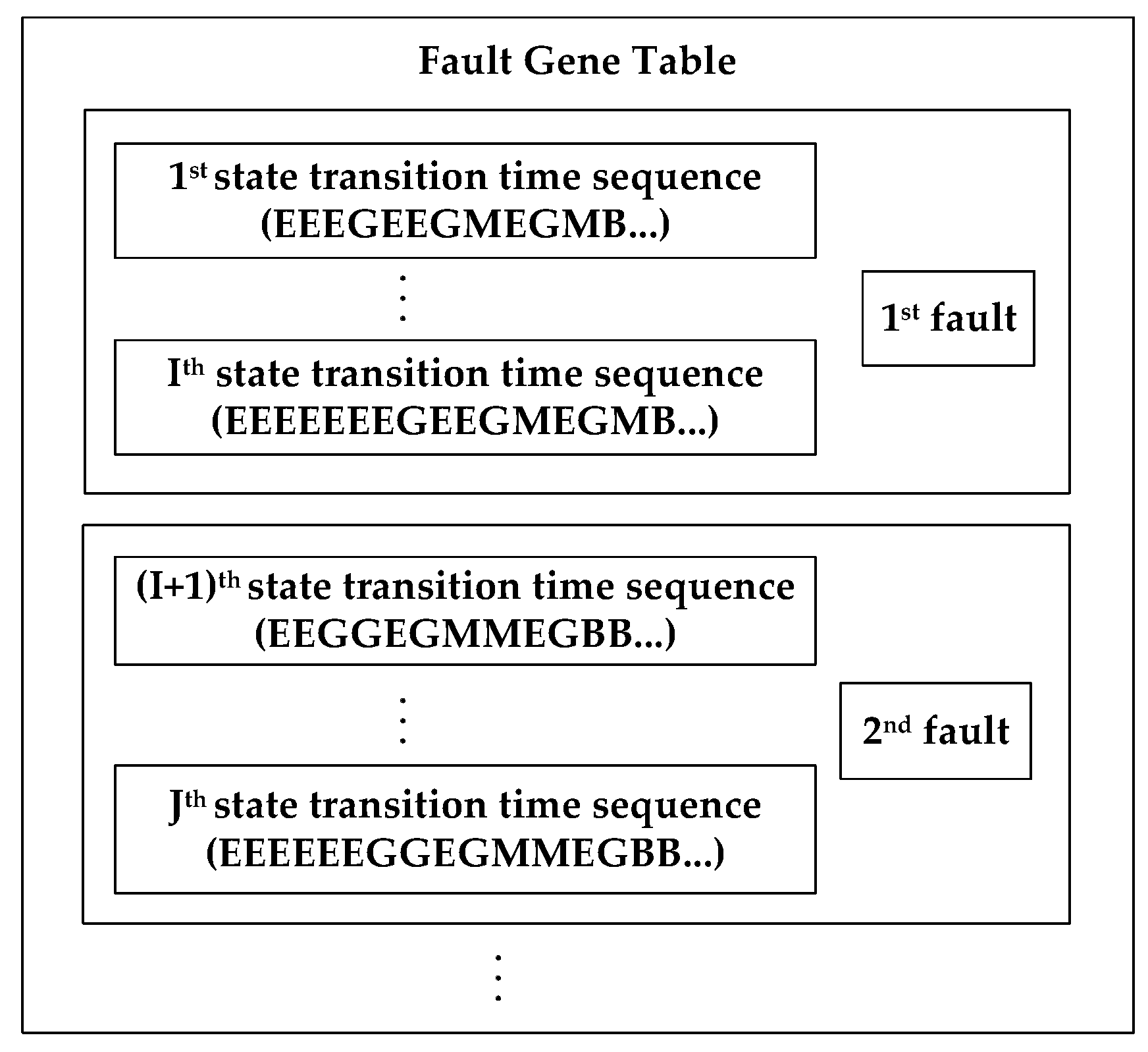
Figure 4.
The block diagram of fault early waning for smart distribution grid.

Figure 5.
IEEE-14 bus.
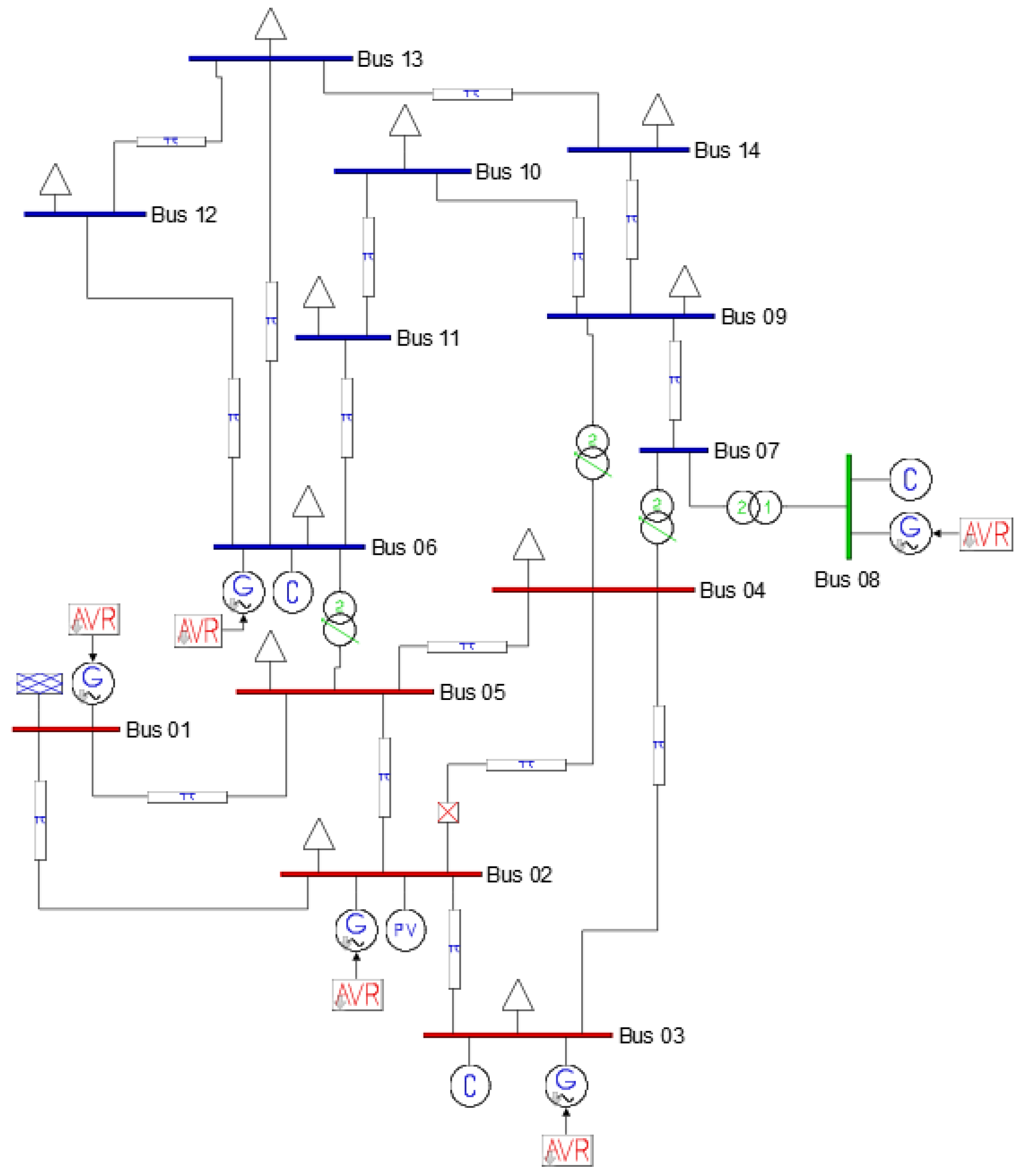
Figure 6.
Three parameters of each bus without disturbances: (a) Voltage; (b) Active power; (c) Reactive power.
Figure 6.
Three parameters of each bus without disturbances: (a) Voltage; (b) Active power; (c) Reactive power.

Figure 7.
Three parameters of each bus with random disturbances: (a) Voltage; (b) Active power; (c) Reactive power.
Figure 7.
Three parameters of each bus with random disturbances: (a) Voltage; (b) Active power; (c) Reactive power.

Figure 8.
Clustered 166 groups of data with 14 dimension reduces to two-dimensional points.

Figure 9.
Relation between the average accuracy rate of BP neural network evaluation model and the number of neurons in a hidden layer.
Figure 9.
Relation between the average accuracy rate of BP neural network evaluation model and the number of neurons in a hidden layer.

Figure 10.
Flow chat of fault gene table construction for smart distribution grid in the simulation test.
Figure 10.
Flow chat of fault gene table construction for smart distribution grid in the simulation test.

Figure 11.
Typical relationship between sate transition time sequences and component faults in the simulation test.
Figure 11.
Typical relationship between sate transition time sequences and component faults in the simulation test.

Figure 12.
Flow chart of fault early warning for smart distribution grid in the simulation test.

Figure 13.
Relations between the average accuracy rate of fault early warning and threshold in different weights.
Figure 13.
Relations between the average accuracy rate of fault early warning and threshold in different weights.
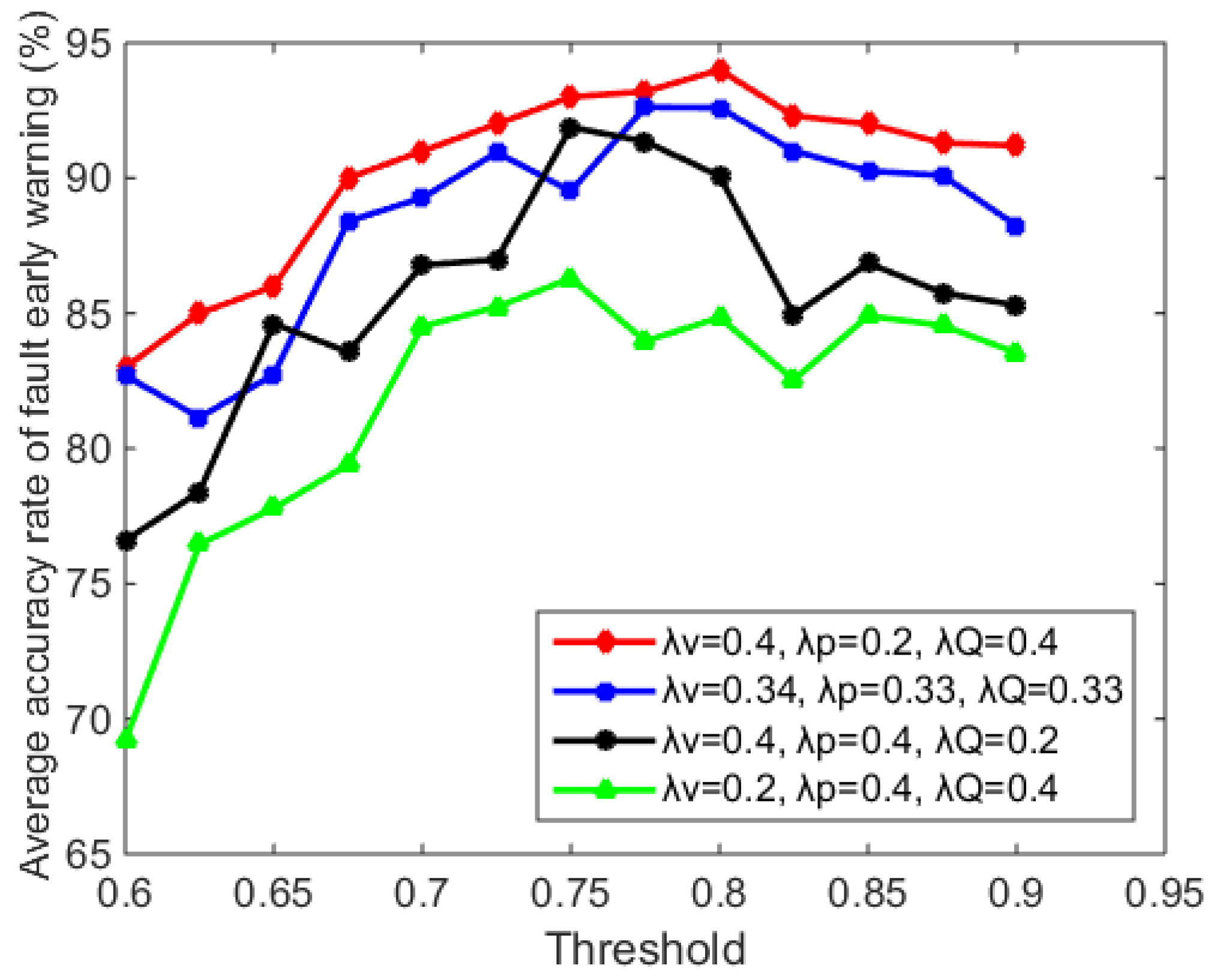
Figure 14.
Relations between the accuracy rate of fault early warning and times of simulation.

Table 1.
State division of smart distribution grid.
| Operational State | Excellent | Good | Middle | Bad |
|---|---|---|---|---|
| Label | E | G | M | B |
Table 2.
Division rule of output state in BP neural network.
| Output | ||||
|---|---|---|---|---|
| State | Bad(B) | Middle(M) | Good(G) | Excellent(E) |
Table 3.
Weights of bus operational state goal.
| Parameters | |||
|---|---|---|---|
| 1st set | 0.34 | 0.33 | 0.33 |
| 2nd set | 0.4 | 0.4 | 0.2 |
| 3rd set | 0.4 | 0.2 | 0.4 |
| 4th set | 0.2 | 0.4 | 0.4 |
Table 4.
Simulation parameters of BP neural network.
| Parameters | Nodes of Input Layer | Nodes of Hidden Layer | Nodes of Output Layer | Learning Rate | Active Function |
|---|---|---|---|---|---|
| Value | 14 | [4,20] | 1 | 0.1 | sigmoid |
Table 5.
Simulation parameters of Smith–Waterman algorithm.
| Parameters | Warning Threshold |
|---|---|
| Value | [0.6, 0.9] |
Table 6.
Importance degree of four operational state in smart distribution grid.
| Parameters | ||||
|---|---|---|---|---|
| Value | 1 | 2 | 3 | 4 |
Table 7.
Model parameters in IEEE-14 bus.
| Model | Bus | Line | Transformer | Synchronous Machine | PQ Load | AVR | Constant Voltage (PV) Generator | Breaker | Static Compensator |
|---|---|---|---|---|---|---|---|---|---|
| Number | 14 | 16 | 4 | 5 | 11 | 5 | 1 | 1 | 3 |
Table 8.
Component faults in fault gene table.
| Component Fault | Bus | Generator | Line | Breaker |
|---|---|---|---|---|
| Fault number | 60 | 50 | 100 | 40 |
Table 9.
Substitution matrix for gene sequence alignment.
| State | E | G | M | B |
|---|---|---|---|---|
| E | 1 | −1 | −2 | −3 |
| G | −1 | 4 | −1 | −2 |
| M | −2 | −1 | 9 | −1 |
| B | −3 | −2 | −1 | 16 |
Table 10.
Comparison of the proposed model with existing models.
| Model | Proposed Model | Based on Harmonic Current [13] | Fuzzy Logic Approach [14] | Bayesian Network [15] | Based on Short Circuit Current [16] | Fuzzy Comprehensive Evaluation and Bayes Discrimination [17] |
|---|---|---|---|---|---|---|
| Considered factors | All buses | harmonic current | Extreme weather | Affected components | short circuit current | Power transformer |
| Can it comprehensively consider the operational state | Yes | No | No | Yes | No | No |
| Is accuracy rate improved with the increase of times | Yes | No | No | No | No | No |
| Data sources | Simulation | Actual data | Simulation | Actual data | Simulation | Actual data |
| Verification means | Simulation | Actual Test | Simulation | Actual Test | Simulation | Actual Test |
| Result | Accuracy rate is close to 97% | Can detect the abnormal changes of the system harmonic current | Accuracy rate is 100% | Provide certain support degree for some faults | Can effectively predict the size of short circuit current | Can effectively discriminate the operational state of power transformer and warn early |
© 2017 by the authors. Licensee MDPI, Basel, Switzerland. This article is an open access article distributed under the terms and conditions of the Creative Commons Attribution (CC BY) license (http://creativecommons.org/licenses/by/4.0/).
Share and Cite
MDPI and ACS Style
Xiang, M.; Min, J.; Wang, Z.; Gao, P. A Novel Fault Early Warning Model Based on Fault Gene Table for Smart Distribution Grids. Energies 2017, 10, 1963. https://doi.org/10.3390/en10121963
AMA Style
Xiang M, Min J, Wang Z, Gao P. A Novel Fault Early Warning Model Based on Fault Gene Table for Smart Distribution Grids. Energies. 2017; 10(12):1963. https://doi.org/10.3390/en10121963
Chicago/Turabian StyleXiang, Min, Jie Min, Zaiqian Wang, and Pan Gao. 2017. "A Novel Fault Early Warning Model Based on Fault Gene Table for Smart Distribution Grids" Energies 10, no. 12: 1963. https://doi.org/10.3390/en10121963
Note that from the first issue of 2016, this journal uses article numbers instead of page numbers. See further details here.