Graphical Diagnosis of Performances in Photovoltaic Systems: A Case Study in Southern Spain

Abstract

The starting point of the operation and maintenance tasks in photovoltaic plants is the continuous monitoring and supervision of its components. The great amount of registered data requires a major improvement in the ways this information is processed and analyzed to rapidly detect any potential fault, without incurring additional costs. In this paper, a procedure to perform a detailed graphical supported analysis of the operation of photovoltaic installations, based on inverter data, and using a self-developed application, is presented. The program carries out the automated processing of the registered data, providing their access and visualization by means of color maps. These graphs allow a large volume of data set to be simultaneously represented in a readable way, enabling operation and maintenance operators to quickly detect patterns that would require any type of intervention. As a case study, the operation of a grid-connected photovoltaic plant located in southern Spain was studied during a period of three years. The average daily efficiency values of the PV modules and inverters were in the range of 7.6–14.6%, and 73.5–94% respectively. Moreover, the presence of shadings, as well as the hours and days mainly affected by this issue, was easily detected.

1. Introduction

According to Solar Power Europe’s report entitled Global Market Outlook for Solar Power 2017–2021 [1], in 2016, there was a record of solar growth as 76.6 GW of solar plants was installed and connected to the grid. That is the largest amount of solar power installed in a year so far, which supposed a 50% year-on-year growth over the 51.2 GW added in 2015. In just a decade, the world’s cumulative solar capacity increased by over 4500%, from 6.6 GW in 2006. The 306.5 GW of total grid-connected PV capacity installed at the end of 2016 generated around 2% of the world’s electricity demand. From today’s perspective, it is expected that the total global installed PV capacity will exceed 400 GW in 2018, 500 GW in 2019, 600 GW in 2020 and 700 GW in 2021 [1].

Although all these solar growth numbers may sound very impressive, solar energy still has a long way to go before it can achieve its full potential, having many obstacles and technical challenges to overcome in order to improve its profitability and to be fully integrated as a dispatchable energy resource in the electricity market [2,3,4,5,6]. The 1.5 °C Paris goal will require gigantic efforts, and, among others, it will need to direct much more money into renewable resources, and new business opportunities may be open in this sector in the near future [1].

Improving the profitability of photovoltaic (PV) installations requires optimizing their production, thus reducing their costs and increasing the plant’s useful life [5,7,8]. To achieve this while still using the currently available technology, a correct design of the installations and an adequate intervention of the services of operation and maintenance (O&M) are crucial [9]. These services are playing an increasing role, and are being recognized for their determining function in ensuring long-term revenues, which is very important when taking into account the current tendency to install, mainly in emergent markets, megawatt-scale PV parks [1,2,7,9]. O&M has even charted its own course to become a standalone business segment and a critical component of the solar energy value chain [1]. Although O&M markets will continue their consolidation in Europe, in emerging markets, ambitious national solar programs are being carried out with few experienced O&M service providers, thus improving these services is one of the challenges for the next few years.

For an adequate intervention of all these O&M activities, the starting point is the continuous monitoring and supervision of both the PV power plant conditions and the performance of all its components [10,11]. An important requirement in this sector is to improve the ways of effectively processing and analyzing the large amount of data registered. In this way, they can be converted into useful information, for faster identification of behavior changes that might compromise the systems’ performance and for faster intervention at the plant if necessary [7,12]. In addition to technical activities, the financial aspects of these tasks are crucial in order to identify and accomplish the appropriate actions in an optimal mode, based on a cost-benefit analysis, with the objective of these services being profitable for both the companies carrying O&M services out and for the owners of the PV installations [12]. Optimal operations must strike a balance between maximizing production and minimizing cost [7].

In this context, the main objective of this paper was to implement a procedure to perform a detailed graphical supported analysis of the operation of PV installations, using a self-developed application named S·lar2. This software enables us to carry out a detailed performance study of all PV plant’s components in a fully automated way. To do this, it calculates the behavior indexes and loss rates of the PV system components [13,14,15,16,17] using data recorded by the inverters, having previously provided all technical specifications of the plant. All parameters analyzed were graphically represented in the form of color maps, boosting the application of advanced data visualization (ADV) techniques [18,19,20,21,22,23] and improved interfaces and decision support (IIDS) tools [24] in the analysis and management of energy production in PV plants. With this type of data visualization, very easy and intuitive information about the behavior of panels and inverters, as well as possible deviations from normal operation or anomalous situations, can be obtained at a glance. The instants of time at which such events take place can be quickly detected. Using this procedure, the operation of a grid-connected PV plant located in southern Spain was analyzed in detail during a period of three years.

The diagnosis of the operating mode and fault detection in PV plants is increasingly attracting the interest of researchers [25,26,27,28,29,30,31], and numerous papers have been published in the last few years dedicated to analyzing the operation and performance of the components of working PV plants [4,32,33,34,35,36,37,38,39,40,41,42,43,44,45,46,47,48,49,50,51,52,53]. Compared to most previous publications, where usually only the daily and/or monthly values of yield and loss indexes are represented, layering the data on a color map allows simultaneously displaying all instantaneous data registered throughout the monitoring period, even if it comprises several years, easing the comprehension and interpretation of large amounts of data. Large-scale visualizations would enable O&M operators to quickly detect patterns in data that would otherwise go unnoticed, helping to close the gap between information and insights, and facilitating diagnostics or alarm management with a minimal effort. This would allow decision-makers to act as quick as possible. Moreover, this procedure does not include additional economic costs since data recorded by the inverters themselves are used.

The structure of the paper is organized as follows. Section 2 describes the magnitudes to be analyzed and the procedure carried out by the developed software. Section 3 describes the characteristics of the grid-connected PV plant analyzed as a case study. Section 4 presents and discusses the results, and, finally, the conclusions obtained in this paper are exposed in Section 5.

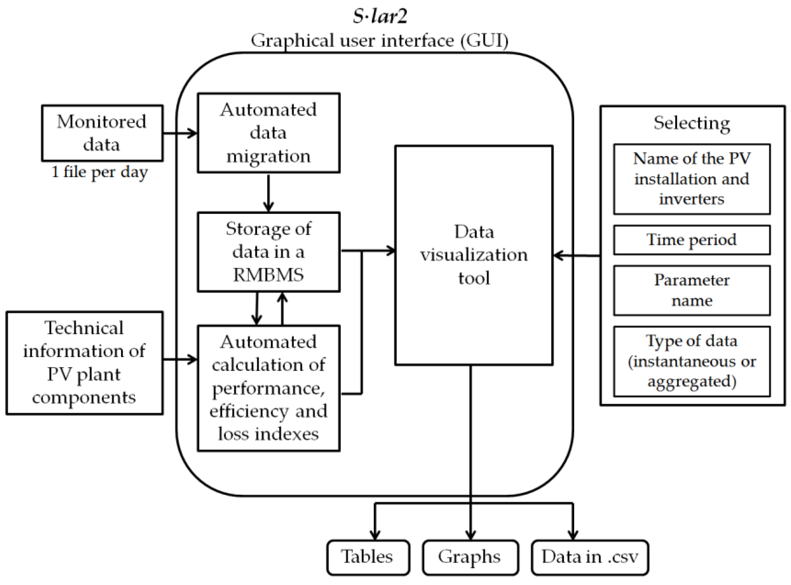
2. Functionalities Included in the Software S·lar2

In this section, the parameters involved in the study are described, as well as the most important characteristics of the software used and the procedure carried out to process and visualize all data.

2.1. Description of Monitored Data and Calculated Parameters

Data monitored by the inverters of a PV plant connected to the grid are shown in

Table 1. Analyzed parameters measured by inverters.

Parameters	Notation
DC current from PV modules	IDC
Inverter input DC voltage from PV modules	VDC
Inverter output AC power	PAC
Inverter output total energy	EAC
AC current injected into the grid	IAC
Grid current	Igrid
Grid AC phase voltage	VAC
Grid frequency	fgrid
Inverter operating status	Status
Inverter error code	Error

. The values of the irradiance in the plane of the PV panels, G, the ambient temperature, T_a, and the temperature measured on the back surface of the PV modules, T_m, were also recorded.

With these measured data, while also using technical information of the plant, a series of standardized behavior magnitudes and rates must be calculated in order to analyze the performance and losses of each of the installation components [13,14,15,16,17,54].

On the one hand, the so-called reference, Y_r, temperature corrected, Y_T, array, Y_A, and final yields, Y_F, were determined. The reference yield is defined as

Y_r = E_G/G_STC

(1)

where E_G is the tilted irradiation, determined by multiplying the value of the in-plane irradiance, G (W/m²), by the monitoring time interval expressed in hours, t (h). G_STC = 1000 W/m² is the irradiance in STC standard conditions (AM1.5, 1kW/m², 25°C). The reference yield represents the time that radiation should be received by the PV array with a value of G_STC = 1000 W/m² in order to generate E_G [13,17,33,54]. Its value depends on the location, orientation and inclination of the PV system as well as on the climate and weather conditions.

The reference yield corrected by the effect of temperature is determined by means of the expression

Y_T = Y_r·[1 − c_T(T_c − T_STC)]

(2)

where T_c is the PV cell temperature (°C); T_STC is the temperature at STC, 25°C; and c_T is the temperature coefficient of the PV modules (%·°C⁻¹), given by the manufacturer in its specifications. This expression reflects the decrease of the production due to the modules’ PV cells work with a temperature above 25 °C. The values of T_c were determined using the expression

T_c = T_a + (G/800)·(T_INOCT − 800)

(3)

This is the most frequently used NOTC model to determine the value of T_c [4,29,37,47,53,54,55,56,57,58,59], but, in this case, the parameter T_INOCT is used instead of the normally used T_NOCT. This latter value is defined as the Normal Operating Cell Temperature (NOCT) and represents the mean PV cell junction temperature in the so-called Nominal Terrestrial Environment (NTE) conditions (ambient temperature T_a,NTE = 20 °C, wind speed v_NTE = 1 m/s on the front and back sides of the PV module and irradiance G_NTE = 800 W/m²) in an open-rack mounted, open-circuit module tilted perpendicular to the solar noon. The T_NOCT should characterize the module’s temperature dependence and should allow the estimation of the module’s performance and energy yield over time [60]. The value of T_NOCT is provided for standard conditions by the module manufacturer in its specifications, while the parameter T_INOCT is defined taking into account the particular shape in which the panels have been mounted and oriented, which may not be the same used by the manufacturer for T_NOCT measurements in the laboratory. The parameter T_INOCT depends on the value of T_NOCT and the configuration used in the installation to mount the PV panels [61]. For the case of open-rack mounting, which is the case of the installation analyzed in this work, T_INOCT is given by the expression [62,63]

T_NOCT = T_INOCT − 3 (°C)

(4)

Greater differences between both temperatures are found in the case of panels integrated directly in façades or building roofs, where the variation between both can be up to 18 °C [62,63,64].

The array yield is defined as

Y_A = E_DC/P_STC

(5)

where E_DC is the DC energy from the PV modules, determined from the DC current and voltage from PV panels multiplied by the recording time interval expressed in hours, t, and P_STC is the PV nominal power under standard conditions measured in W. This quantity represents the time in which the PV generator must be operating with nominal power P_STC to generate E_DC energy [13].

The final yield is determined by

Y_f = E_AC/P_STC

(6)

where E_AC is the AC energy from inverter, determined from the monitored inverter output AC power, P_AC, and the recording time interval expressed in hours, t (h). This quantity represents the time in which PV generator plus the inverter must be operating with nominal power P_STC to generate E_AC energy [13]. It depends on the location and type of installation, so it enables one to compare the production of similar PV installations with different sizes but located in a specific geographic region.

Calculating the differences between the previous parameters, the losses of the different components may be determined. The array capture losses may be calculated as the difference between the reference and the array yields as

L_c = Y_r − Y_A

(7)

Capture losses are given by the sum of thermal losses, L_ct, and miscellaneous losses, L_cm. The thermal capture losses are determined by the difference between the reference yield and the temperature corrected reference yield

L_ct = Y_r − Y_T

(8)

and represent the losses due to PV modules that are operating above 25 °C [62]. The miscellaneous capture losses are determined by means of the difference between the temperature corrected reference yield and the array yield, and it is given by

L_cm = Y_T − Y_A

(9)

It represents the rest of the losses in the PV system, which may be associated with multiple causes such as the Joule effect in the wiring, diodes losses, shading effects, inhomogeneous or low irradiance, snow, contamination or dirt accumulation, mismatch, maximum power tracking error, etc. An incorrect operation of a PV grid-connected installation leads to a significant increase in L_cm value, being this magnitude an indicator of the existence of problems in the system. Finally, the difference between the array and the final yields is given by

L_s = Y_A − Y_f

(10)

which corresponds to the losses produced in the inverter.

The performance ratio, expressed by the ratio of the final and reference yield

PR = Y_f/Y_r

(11)

is a dimensionless index mainly used to characterize the performance of PV installations, which measures the degree of utilization of an entire PV system [65,66]. It is the ratio of useful generated energy versus the energy that should be generated by a lossless ideal PV plant at 25 °C and receiving the same irradiation. This parameter was defined in the recently revoked standard IEC 61724:1998 [16], and it is considered with more detail in the recently published standard IEC 61724-1:2017 [17]. It takes into account all the effects that involve the PV system performance and indicates the overall effect of losses on the PV system’s rated output due to array temperature, incomplete utilization of the irradiation and system component inefficiencies or failures [16,33,65].

For determining the global value of PR for a PV installation, Y_f must be determined using the E_AC values measured at the PCC by the meter installed by the electric company [65]. However, in this work, the objective is to be able to compare the operation of the three inverters available in the PV installation. The PR value of the ensemble formed by each inverter of the installation, together with the PV array connected to it, was determined, and, for this, the value of E_AC registered by the inverters was taken into account for determining the value of Y_f for each inverter. In this case, the losses that would take place between the inverter and the meter were not considered in this work.

The temperature-corrected performance ratio, PR_T, was defined by the IEC 61724-1:2017 [17]. In this case, instead of using the value of the final yield previously defined, the value of a corrected temperature final yield, TC_Y_f, defined as follows, will be used

TC_Y_f = E_AC/(P_STC·[1 − c_T(T_m − T_STC)])

(12)

Instead of using a constant value of P_STC, the reference power is calculated at each recording interval to compensate for the differences between the actual module temperature (T_m) and the STC reference temperature of 25 °C. The standard IEC 61724-1:2017 [17] indicates that, in this case, the measured module temperature T_m may be used.

The efficiencies with which the components of the installation are working were also determined. The efficiencies of the PV modules were calculated by means of the expression

η_G = (E_DC/E_r) × 100

(13)

where E_r is the reference energy calculated by the product of the tilted irradiation, E_G, by the PV module area associated to each inverter, A [54]:

E_r = E_G·A

(14)

This reference energy represents the available irradiation on the total PV module surface. The efficiency of the inverter was determined by the ratio of the AC energy from inverter versus the DC energy from PV modules:

η_inv = (E_AC/E_DC) × 100

(15)

It depends on the input voltage to the inverter (some inverters operate more efficiently in the upper area of the MPP voltage window, while other manufacturers prefer the lower, and even some choose the intermediate zone). This should be taken into account when choosing the number of modules in the series associated to each inverter [67].

Finally, the system efficiency, given by the product of the inverter efficiency and the efficiency of the PV modules associated with it,

η_s = (η_G·η_inv)/100

(16)

provides the efficiency of the system composed by both of them. In the case of installations with more than one inverter, these magnitudes can be determined for the systems comprised by each inverter and its associated PV modules and/or for the complete installation, adding or multiplying the results for each inverter, as appropriate.

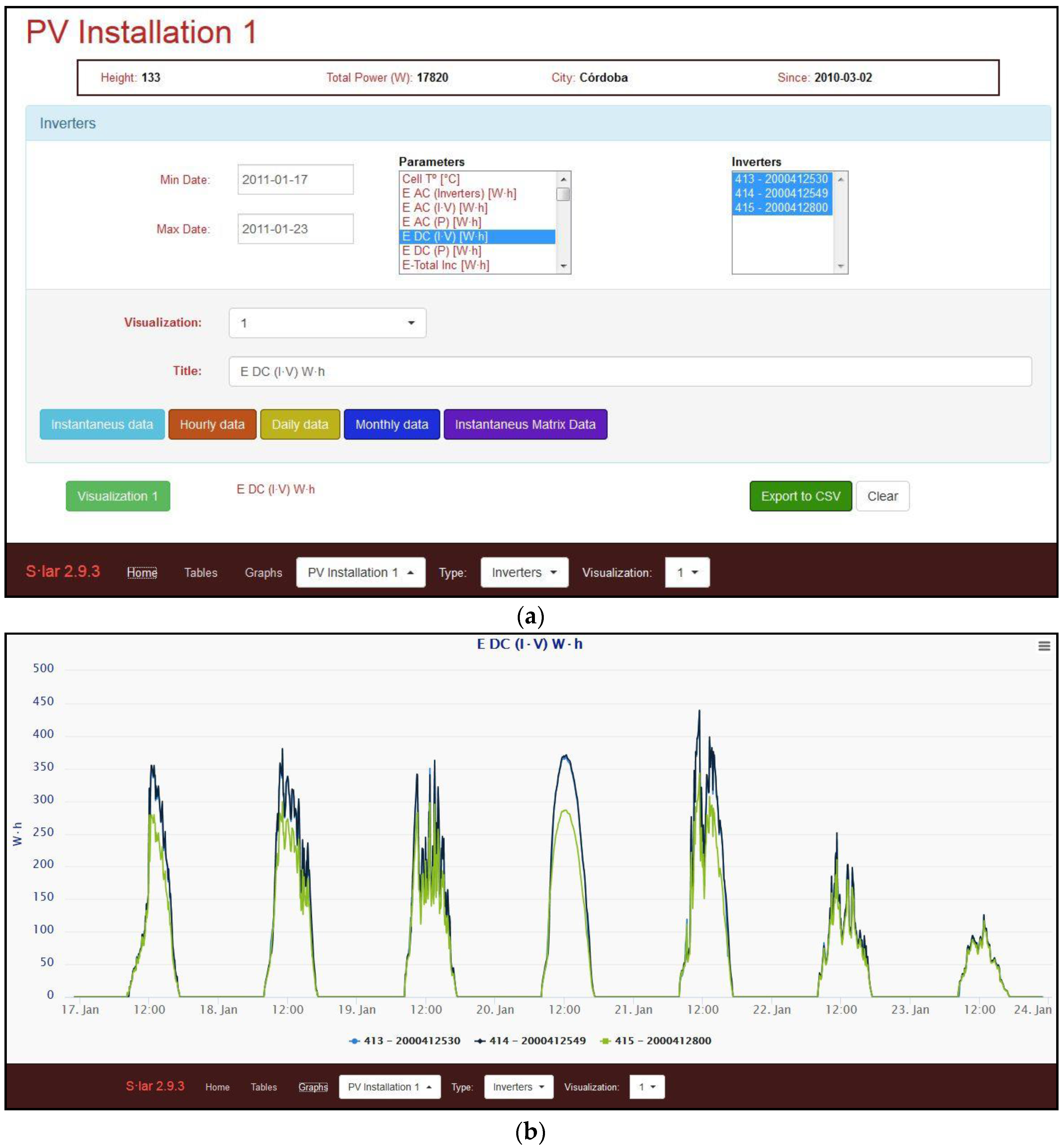
2.2. Description of Data Processing and Visualizing Procedure

The management and processing of the monitored data were carried out using our self-developed software S·lar2. This software was specifically designed for the automatic reading, management, treatment and storage of data measured in PV installations. A previous version of this software was the objective of the study in a previously published work [54], where it was described in detail. In the new version, this software was modernized to a web application, more flexible to be installed on the customer's equipment, and with shorter processing and consulting times. It was developed using Python [68], HTML [69], CSS [70] and Typescript [71].

Figure 1 shows a schematic diagram where the steps that are carried out in the developed program for processing and visualizing the information are reflected. The monitored data of the PV installation, as provided by the company which are the owner of the plant, are distributed in one file per day and organized in directories by months and years. S·lar2 enables monitoring data to be automatically entered into different tables in a Relational Database Management System (RDBMS), specifically designed to contain all of this information. The application has a graphical user interface (GUI) that facilitates data migration and all their processing. Once all recorded data have been stored, the software allows for performing a series of mathematical operations on the monitored parameters for the calculation of Equations (1)–(16) for each inverter. Therefore, each of the previously shown standard magnitudes and performance rates of each individual component of the PV installations can be calculated and stored.

Moreover, the application determines both the “instantaneous values” of all parameters and calculated magnitudes, which will have the same temporal frequency as the recording parameters, and all of their average and/or accumulated or aggregated values, which are also automatically calculated. These last values must be calculated to produce an hourly scale (the sum or average of the instantaneous values recorded or calculated for each hour), a daily scale (sum or average of the 24-hourly values for each day), and a monthly scale (sum or average of the daily values for each month).

Once data are calculated, the S·lar2’s graphical user interface (GUI) also enables the user to easily access and select all data stored in the databases, by means of a series of queries via its data visualization tool. A screenshot of this data visualization tool can be observed in Figure 2a. By means of a series of buttons and menus, selected data can be directly visualized either graphically (Figure 2b) or numerically, in tabular form, or even being exported as .csv files with the aim of using them with other third-party software for its analysis.

The PV installation was analyzed as a case study during a period of three years (from 1 January 2011 to 31 December 2013), for which the monitored data of the installation were available. The 1096 files, which contain the parameters recorded by the three inverters as well as the irradiance and temperature data, were provided by the company that owns the facility. These files were then uploaded using the software and subsequently calculating all the yield and loss indexes. By using the developed application, the same parameters for the three inverters were queried.

For the analysis, all the instantaneous data of each parameter were represented in the form of color maps. With this type of data visualization, a large volume data set can be represented in a readable way, easing its interpretation, and with the aim of assisting in the decision-making process of PV plant maintenance tasks. To do this type of representation, in S·lar2, the option has been added to request for any of the parameter’s data in a matrix form. The application will supply us data in an array that will have as many columns as the requested days corresponding to the monitoring period, and as many rows as records have been made throughout each day. The days in which, due to technical problems, there are no monitoring data, the program provides the columns corresponding to those days with null or empty values, according to interest. Since the PV installation has been analyzed in this work during a period of three years, there were 1096 columns in total in these matrices, but obviously the matrix’s number of columns can be adjusted to the number of days in which this analysis of the PV installation is desired to be done. On the other hand, for a recording interval of 5 min, as is the case of the PV installation analyzed in this work, there are 288 data recorded per day for each parameter, so this will be the number of rows that the matrix will have: the first data or row being the one corresponding to the registration at 00:00, and the last one corresponding to the registration at 23:55. Then, the data of these matrices will be represented by color diagrams. In the Y-axis, the 288 registers or rows are represented, while the X-axis shows the monitored days, or the different columns that the matrix have, which is the same. The magnitude of the values will be given in such graphical representations by a color scale.

Graphs with daily data, which will correspond to the sum or average of the values of each of the matrix’s columns, will be presented after the color maps, such that the union of both graphs will provide complete information of each parameter analyzed.

Although S·lar2 carries out the graphical representations of the data, in this work the .csv files provided by the software was exported and loaded into MATLAB (version 2013, MathWorks, Natick, MA, USA), with the aim to provide high-quality figures in the paper. By means of a routine, instantaneous data matrices and daily data vectors were uploaded, and all figures were represented in an automated way.

3. Specifications of the PV Plant Analyzed for the Case Study

In this paper, a grid-connected PV system currently operating in Andalusia, Spain, was analyzed. This installation belongs to the company Solar del Valle SL, which provided both the installation’s technical specifications and the data obtained from monitoring [72]. This facility is located in the city of Córdoba (Cordova), with a nominal power of 17.8 kW. It comprises three inverters, each one with 36 modules connected to it (three parallel strings with 12 modules in series each one). The parameters of its modules, mounted in an open rack on a rooftop (tilt: 30°, azimuth: 18°), are shown in

Table 2. PV module technical specifications.

PV Module	Specifications
Model	BP-3165
Type	Polycrystalline Silicon
Number of cells	72 (6 × 12)
Nominal power (PSTC)	165 W
Power tolerance	±3%
Module efficiency	13.1%
Maximum power current (Ipm)	4.7 A
Maximum power voltage (Vmpp)	35.2 V
Short circuit current (Isc)	5.1 A
Open circuit voltage (Voc)	44.2 V
NOTC	47 ± 2 °C
Module area	1593 × 790 × 50 mm
Weight	15.4 kg
Top side	Tempered glass
Encapsulating material	EVA
Back side	White polyester

, whereas inverter specifications are listed in

Table 3. Inverter specifications.

Inverter	Specifications
Model	SMA SMC-5000 [73]
Input
Recommended Maximum DC power	6.35 kWp
Maximum DC voltage	600 V
Maximum DC current	26 A
Nominal DC voltage	270 V
Output
Nominal AC power	5 kW
Maximum output current	26 A
THD of grid current	<4%
Number of phases	1
Maximum efficiency	96.0%
Euro-eta	95.1%
Weight	63 kg

. The three inverters of the PV installation has been named inverter 413, inverter 414 and inverter 415, which are labels used by the owners of the plant.

Monitoring was carried out in the PV installation with the following equipment. In-plane irradiance and temperatures were recorded by using a device called Sunny SensorBox, from the SMA company [73], whose sensors and specifications are reflected in

Table 4. Irradiance and temperature sensors.

Sensor	Measurement Range	Accuracy	Resolution	Magnitude Measured
Calibrated ASI amorphous PV cell	[0,1500] W/m2	±8%	1 W/m2	In-plane total irradiance on the PV modules (it is located close to one of them, with the same inclination and orientation)
PT-100M	[−20,+110] °C	±0.5 °C	0.1 °C	Module temperature
PT-100M-NR	[−20,+110] °C	±0.7 °C	0.1 °C	Ambient temperature

. The other measurement sensors and the data acquisition system were located in the inverters. The Sensor Box and inverters were connected via RS485 to a Sunny WebBox, also from SMA. This multifunctional device, with a low-consumption data logger, is responsible for collecting data continuously from inverters and the SensorBox. Measurement data are transmitted through a GSM modem from remote locations where a telephone or ADSL connection is available. In the installation, monitoring data, recorded at 5-min intervals in the WebBox, were extracted via an SD card.

4. Results

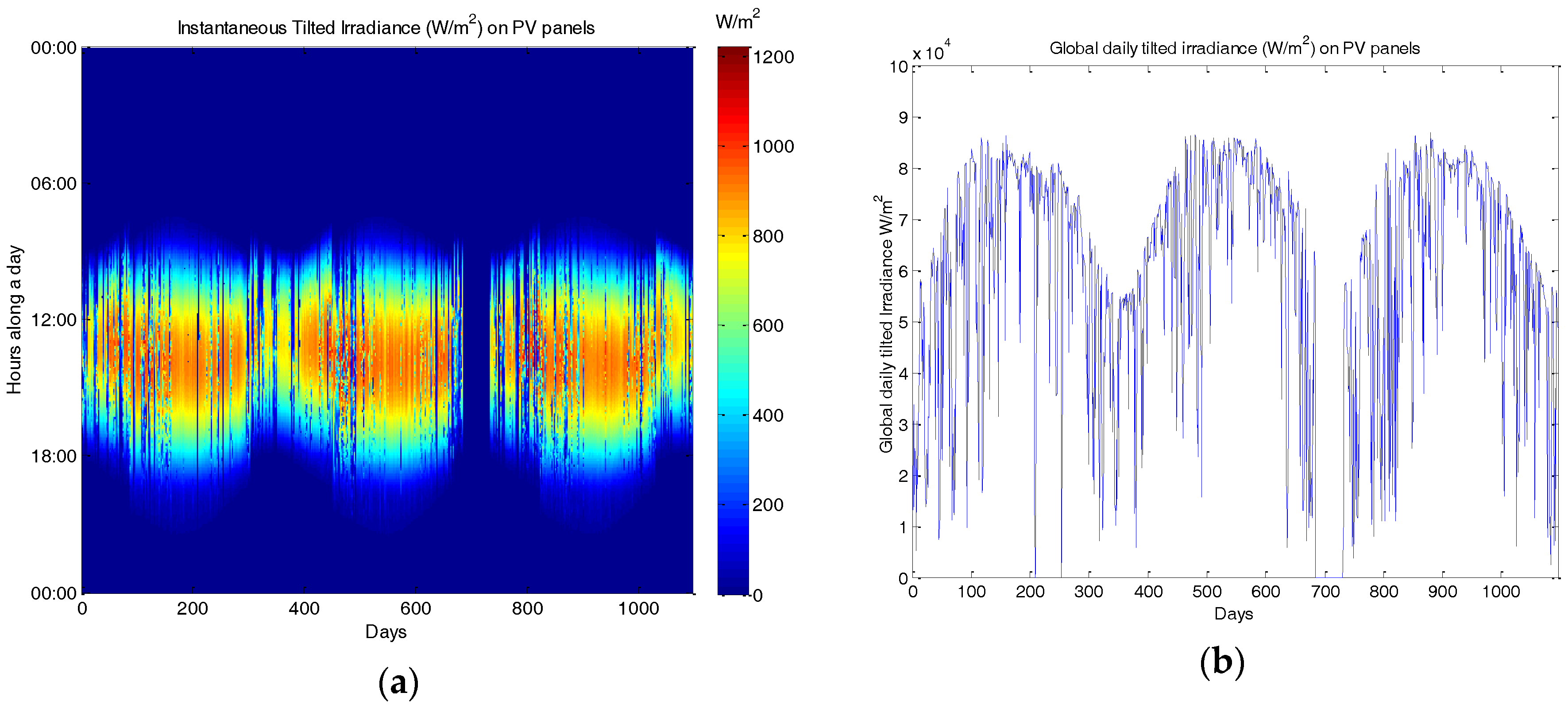
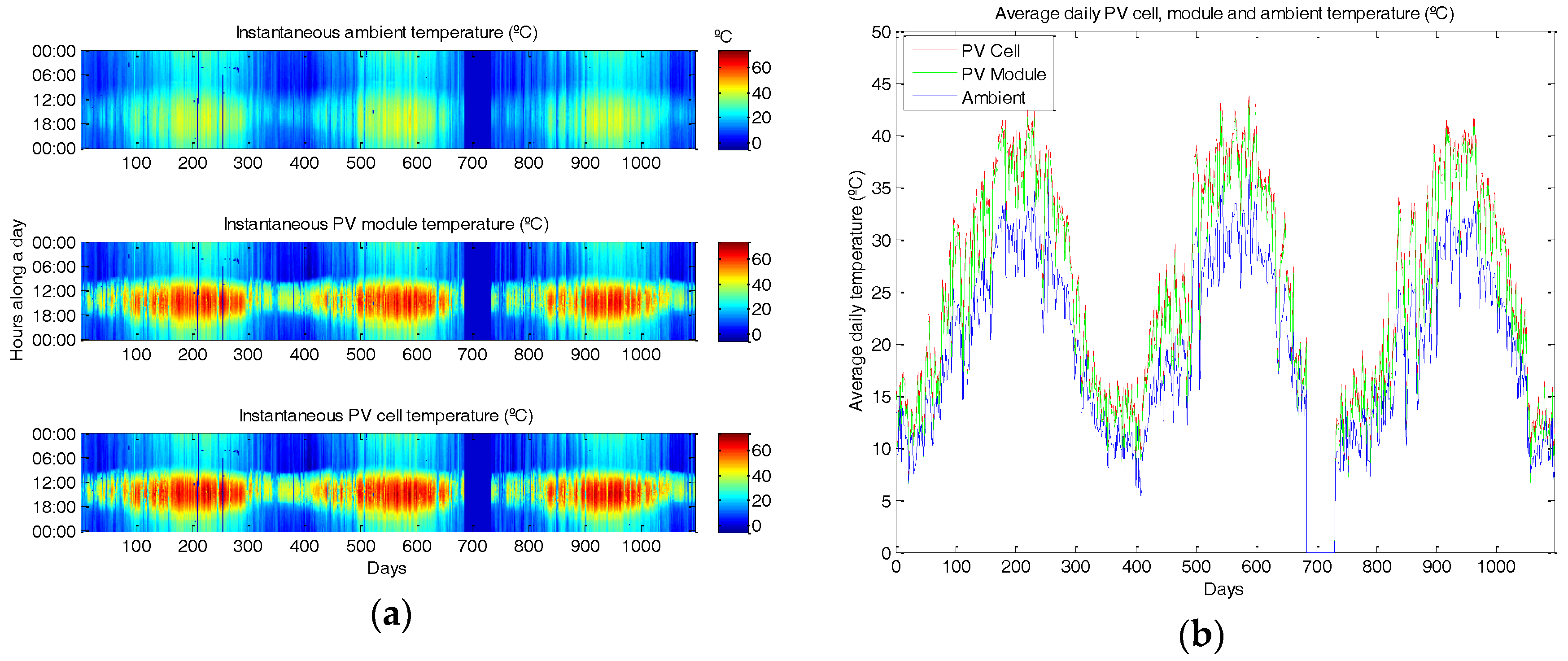
4.1. Irradiance, Ambient and Module Temperature

Firstly, the external parameters of irradiance and temperature to which the PV modules were subjected to are shown in order to have them as a reference to the dependence of the production indices and losses with these parameters. In Figure 3a the tilted irradiance registered during the monitored period of three years is represented. The first day corresponds to 1 January 2011, whereas the 1096th day corresponds to 31 December 2013. Firstly, it is notable that the set of 315,648 records over the three years (288 records per day for 1096 days) is represented on the same graph, and the set of all data is easily interpretable at a glance. The Y-axis shows the hours of the day in which the registers take place, from 00:00 to 23:55, which correspond to the first and last data measured each day. It is possible to observe the seasonality of the irradiance values for the geographic location as well as for the inclination and orientation of the PV panels of the studied installation. In dark blue color, the null values and the instants of time in which there is no record of irradiance, either because it corresponds to night hours or because of the absence of data for some type of technical problem, can be seen. The dark red color corresponds to the maximum values of irradiance. The maximum recorded value was 1141.6 W/m², which took place on 14 April 2012 at 13:50. It is observed in the graph that the months of January and December are the period of the year in which days have the lowest number of hours with non-zero values of irradiance. The hour daily range with solar radiation increases progressively until the summer months, where the number of hours with sun and therefore electricity production is the highest. It can also be observed that the greatest irradiance records take place during the central hours of the day, between 12:00 and 15:00. The two time changes that take place throughout each year in Spain, in the passage from winter to spring (around the end of March), in which there is an advance of 1 h (from Greenwich Mean Time (GMT)+1 to GMT+2), and the transition from summer to autumn (at the end of October), where there is a delay of 1 h (From GMT+2 to GMT+1), are also reflected in the image.

It is observed in Figure 3a, as well as in many others of the work, the range of days, between 14 November 2012 and 1 January 2013 (Days 684–731), in which there was no data in the PV plant´s monitoring system due to technical problems, as well as 26–28 July 2011 (Days 207–209), in which there was also fault in the data.

In Figure 3a, it is possible to observe the difference between the irradiance profiles that occur on clear cloudless days, in which the variation experienced by irradiance values throughout the day is exclusively due to variations in the solar path, with respect to the days with clouds passing, in which, from some registers to others, there were great variations in the values of the irradiance. It can also be observed in those covered days that the values of irradiance were very low throughout the day.

The correspondence between the data of Figure 3a and those reflected in Figure 3b, where the total daily values of irradiance are represented, can be observed. In Figure 3b it is shown, in addition to the annual periodicity that takes place due to the seasonality, already reflected in Figure 3a, the great variation that can take place from day to day in the total daily values of irradiance, present in general throughout all the seasons, although this variation is inferior in summer due to a greater predominance of clear days. This fact results in a great variability and randomness in the production of energy in this type of renewable installations, and therefore in their difficulty to be considered as manageable energy generation sources in the electricity markets. The higher daily total values, above 80 kW/m² per day, were concentrated between the months of April and July. The highest total daily value corresponded to 29 May 2013, with a total of 86.89 kW/m². In contrast, in the months from January to December, the total daily irradiance values were generally the lowest. In these months, the highest total irradiance did not exceed 55 kW/m² per day. Although, as can be observed, it was possible in summer to find days with a total irradiance collected by the panels of less than 55 kW/m², this may be less than 10 kW/m² in winter days.

The ambient, the measured at the back of the modules, as well as the estimated PV cell temperatures are reflected in Figure 4a. The color maps allow an intuitive visualization of the temperature distribution over the three-year period. The average daily values of these three temperatures are shown in Figure 4b. These figures show the seasonality of these three magnitudes, with values being very high in summer, greater between 12:00 and 18:00, and lower in winter, mainly in the months of January and December. The highest registered ambient temperature value, 48.23 °C, took place on 10 August 2012 at 15:15, while the lowest value, −1.17 °C, was recorded on 5 February 2012 at 8:05. The highest values of module and cell temperatures obtained, 73.15 °C and 75.38 °C, respectively, also took place on 10 August 2012 at 15:05, while the lowest values, −5.25 °C and −5.23 °C, respectively, were recorded on 12 February 2012 at 8:15.

The high temperature of the PV modules, being an average of 4.44 °C above the ambient temperature is worth noting. The maximum increase of the module temperature compared to the registered ambient temperature was of 35.96 °C, which was registered on 11 April 2012 at 13:40, while the maximum variation in which the temperature of the module was lower than ambient, 6.6 °C, took place on 13 June 2012 at 7:35. The mean difference found between T_c and T_m is 0.57 °C, although the maximum temperature difference obtained between the both values was 3.43 °C, also recorded on 11 April 2012 at 13:40. The average ambient temperature values range from 5 °C to 36 °C, between 6 and 43 °C for the module temperature and between 6.5 °C and 43.7 °C for the cell temperature.

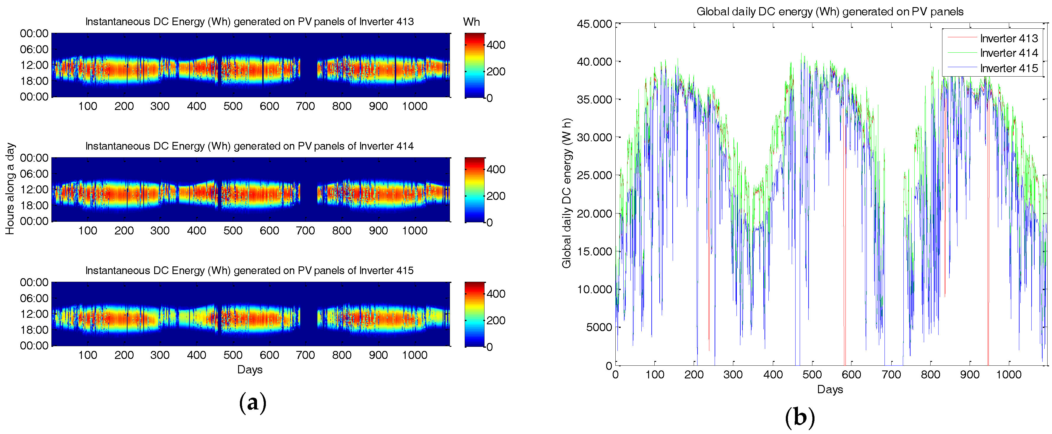
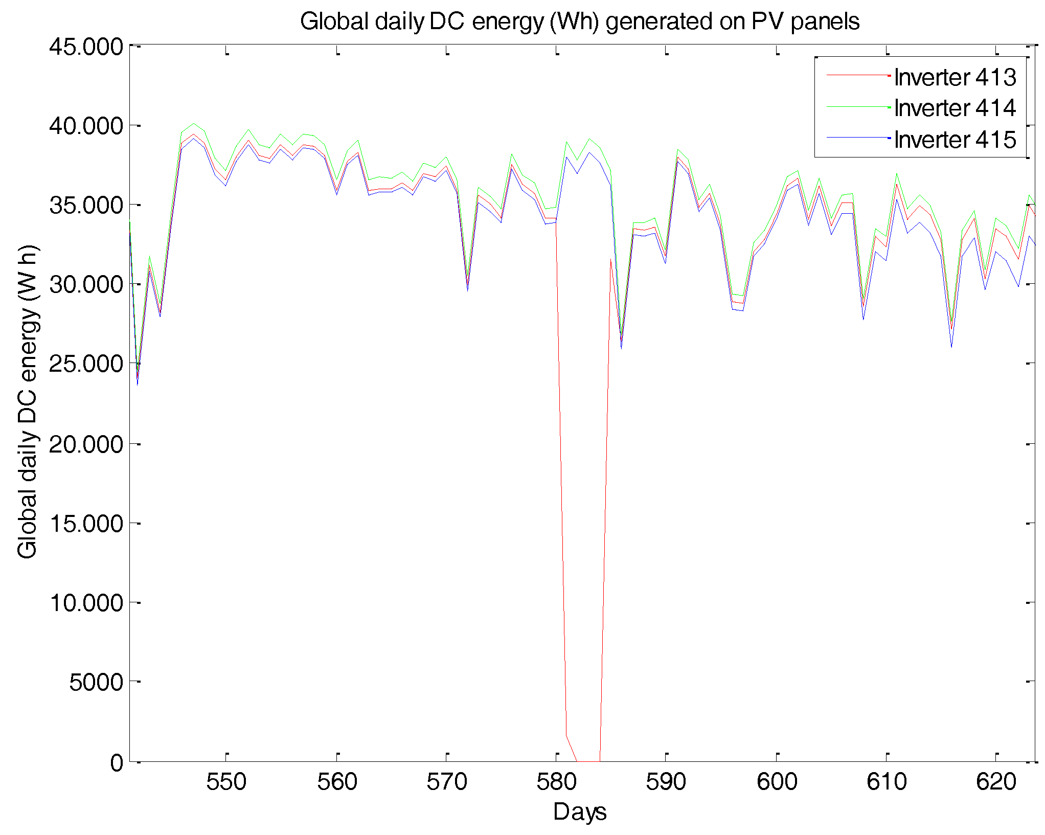
4.2. DC Energy Produced by PV Panels

Once the conditions to which the components of the PV system were exposed to have been shown, in Figure 5a the instantaneous DC energy generated in the PV arrays connected to the three inverters of the installation is represented. The total daily values of this energy are shown in Figure 5b. It can be noticed how the values of this parameter are directly related to the irradiance values received by the panels previously shown in Figure 3a. The seasonality in production over the three years, the highest values of production in the mid hours, the highest number of hours of production in spring and summer, and the differences of the daily DC production profiles on clear days, with small transitions, compared to that of the days with the passage of clouds, with a greater number of transitions, can be observed, all aspects previously commented on when analyzing the color map of irradiance values.

Since the nominal power of panels associated with each inverter is the same, the energy produced in all three should be practically the same. However, if one observes Figure 5a, it can be clearly seen that, in the winter months, during the period from September to March, the electricity output in the arrays connected to inverter 415 is lower than that of the other two inverters. This fact is also shown in Figure 5b, where it is observed that the daily output of the panels corresponding to inverter 415 is lower during these months. The maximum difference occurred on 2 February 2013, in which the daily output of inverter 415 panels was lower by 7.56 Wh than that occurring in inverter 414 panels, which means a daily production that is 24.37% lower. However, the color map allows us to discern, throughout the year, the hours of the day when the production of the third inverter is lower, an aspect that obviously is not evident if only the daily total data are represented.

Figure 5a also shows, during the period from 2 to 12 April 2012 (Days 458–468), a stop in the production of the three inverters, as well as a series of stops that took place only in inverter 413, and that corresponded to 26 June 2011 (Day 238), from 3 to 6 August 2012 (Days 581–584), 17 April 2013 (Day 838) and from 3 to 5 August 2013 (Days 946–948). These stops are also reflected in both Figure 5b and in the enlargement shown in Figure 6. This last figure represents the daily DC energy generated from 23 June 2012 (Day 540) to 15 September 2012 (Day 624). The stop in the production of panels can be clearly seen, which corresponds to inverter 413 from 3 to 6 August 2012 (Days 581–584). It can also be seen that the total daily output of inverter 413’s panels is slightly lower than that of the inverter with the highest production, which is 414, and this difference remains practically constant over the three monitored years. These smaller differences are more difficult to visualize in the color maps, so it is recommended that these maps be accompanied by graphical representations of the daily values in order to complement the information of the first ones. In total, the production of panels associated with inverters 413, 414 and 415, during the three monitoring years, was 28.2, 28.9 and 26.4 MWh, respectively. The output of the 415 inverter was 2.5 MWh lower than that of inverter 414, which is 8.6% lower. This means an average difference between both inverters of 0.83 MWh/year. The difference between inverters 413 and 414 is smaller, 0.7 MWh, which is 2.5% lower. This implies an average difference of 0.24 MWh/year. These differences in the production of the PV panels were reflected in a smaller injection of energy into the grid (0.78 and 0.22 MWh/year respectively for 415 and 413 compared to inverter 414). Considering the remuneration tariff for this type of installations (Type I.1) in 2011 [74], this meant a loss of 245 and 70€ per year respectively for inverters 415 and 413, which despite variations in tariffs, over the plant service life may lead to a considerable decrease in revenues. In the case of inverter 415, this deviation is mainly due to the presence of shading effects.

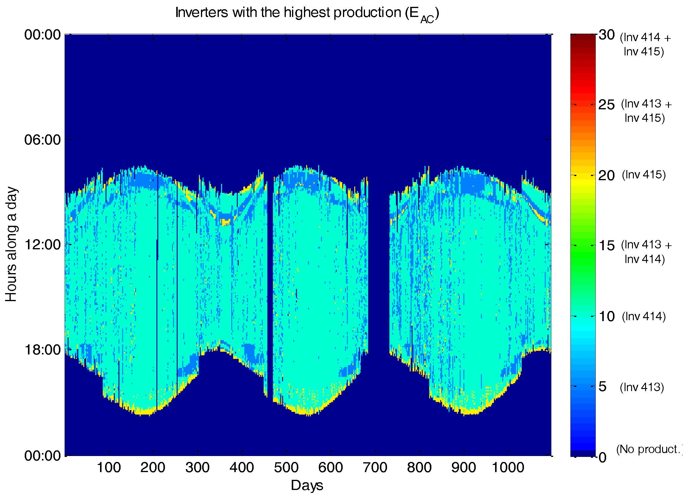
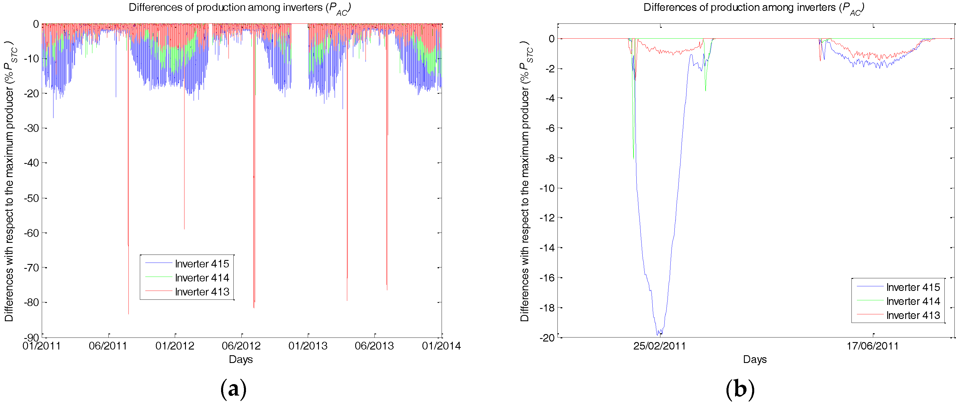
4.3. Maximum AC Energy Produced by Inverters

In this study, the behavior pattern of the instantaneous and total daily energy E_AC measured in the inverters’ outputs are really similar to those of the E_DC represented in Figure 5a,b respectively. Thus, instead, in Figure 7 there is a representation in which, for each instant of time, the inverter with the maximum E_AC energy production is indicated. A code is used, such as 0 (dark blue) means there is no electricity production; 1 (intermediate blue) represents that inverter 413 is producing the maximum value of E_AC in that instant of time; 10 (light blue) represents that inverter 414 is producing the maximum value of E_AC; and 20 (yellow) represents that inverter 415 is producing, in this case, the maximum value of E_AC. The values 15 (green), 25 (orange) and 30 (dark red) would represent the instants of time in which two of the three inverters (413–414, 413–415 and414–415, respectively) are simultaneously producing the maximum amount of E_AC, although these situations are infrequent during these three years. The situation in which the three inverters are producing the same quantity of E_AC, which would correspond to number 35, according to the code used, does not occur during the entire monitoring period. It can be seen that the inverter that is more often producing more energy than the others is inverter 414, which results in the fact that its daily production, as already seen above, is superior to that of the other two inverters in the greater part of the monitoring period. However, it can be observed that the behavior reflected in the figure presents an annual periodicity. The 414 inverter has maximum production during the central hours of the day in the spring and summer months. Inverter 413 produces the most during the first hours of the day, especially during the summer months, and during the last hours of the day, especially during the months corresponding to autumn and winter. In addition, throughout autumn and winter, the maximum production oscillates between inverters 413 and 414. Inverter 415, in a smaller number of occasions, presents the maximum production. However, this occurs during the first and mainly during the last daily production records, but this situation is much less frequent during the central hours of the day.

In accordance with this figure are the data represented in Figure 8. In it, for each of the registers over the three years, the inverter that is having the maximum output has also been determined. Considering that this should be the production expected for the other two inverters, the difference between the output power in each inverter, P_AC, and the maximum output found in the three are calculated for each of them. This difference, in percent, with respect to the value of the nominal power of PV panels associated to each inverter, P_STC, is represented. Figure 8b shows the same values, but on 25 February 2011, as an example of one day in which there are more differences in the production of inverters (around 20%), and on 17 June 2011, as an example of a day in which the difference among the output of the different inverters is the smallest recorded (around 2%). As shown in Figure 7, inverter 414 had the highest production on a greater number of occasions (for that reason, the value corresponding to it in Figure 8b in the central hours of the day was zero), except in some instants of time in the first and last hours of the day, in which the production of this inverter was inferior, thus making inverter 413 the maximum producer in those instants of time.

The influence of some aspects that show a periodicity throughout the year is clearly manifest in Figure 7 and Figure 8, indicating, because the PV installation is located on the roof of a building, the presence of shadows caused by the structure of the building and/or those surrounding it, which is affecting to a greater or lesser extent the production of panels associated with each of these inverters throughout the year. This reduction in production can be improved by rectifying, as far as possible, the design of the PV plant or, at least, by taking this aspect into account in other future installations in which similar circumstances may occur. If rectification is not possible, at least they are foreseeable variations that can be considered in a possible management of the production of the analyzed PV plant.

On the other hand, the presence of faults, for example, in inverter 413, is clearly shown in Figure 8a with differences in the output, which may be even greater than 80% of the nominal power of the array. There are numerous authors who model the production of the PV plant and compare the actual production with that obtained by the model in order to verify the presence of faults in the installation [25,26,27,28,29,30,31]. Another option is, as presented in this work, to compare the production of arrays that are located together and exposed to the same conditions. The deviation in the production of one of them with respect to the others is a sign of the presence of some type of disturbance that is affecting the production. Obviously, this method does not allow for detecting deviations that are simultaneously affecting the output of all inverters, but it avoids having to use a model of both the array and the inverter, whose results will also present errors with respect to the actual production, which is higher the more simplified the model used is. Once the behavior of each inverter has been characterized, alarms can be set for deviations higher than those normally detected for each time of the year in order to control possible anomalous deviations.

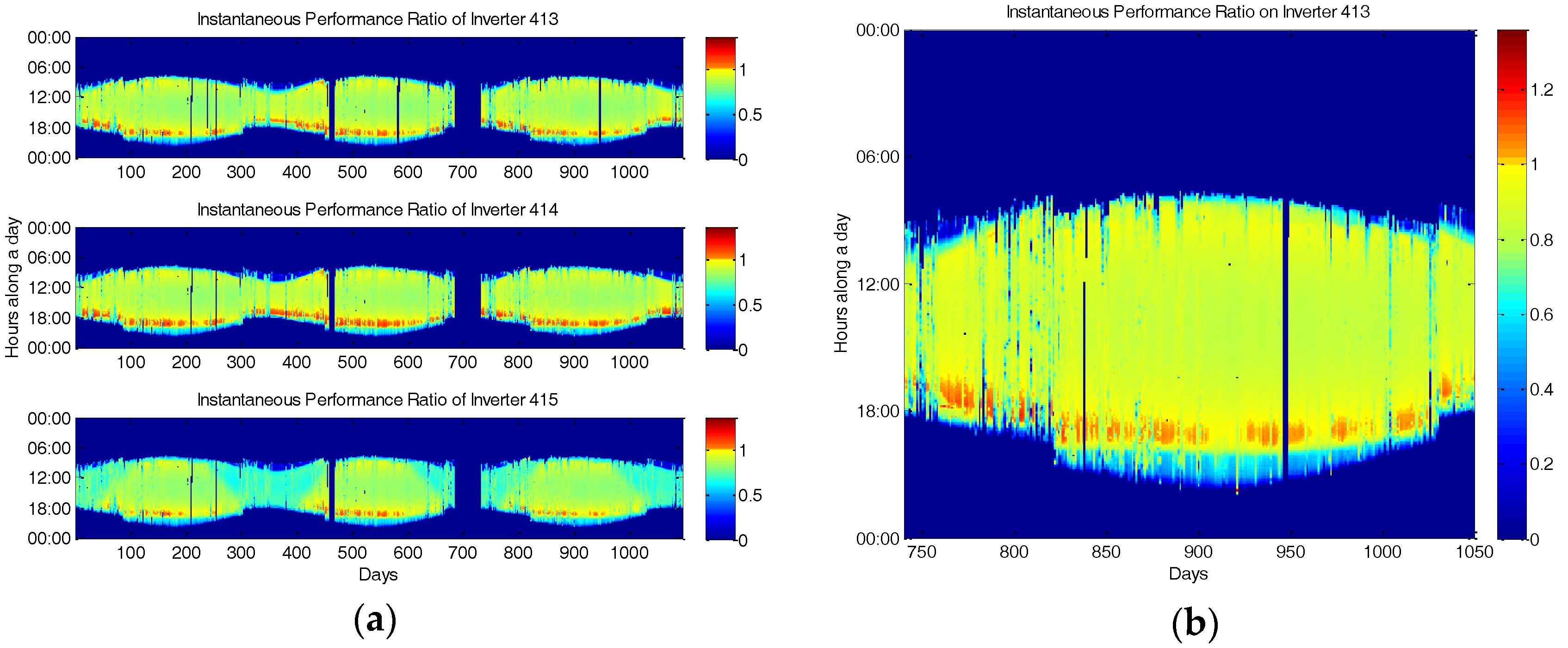
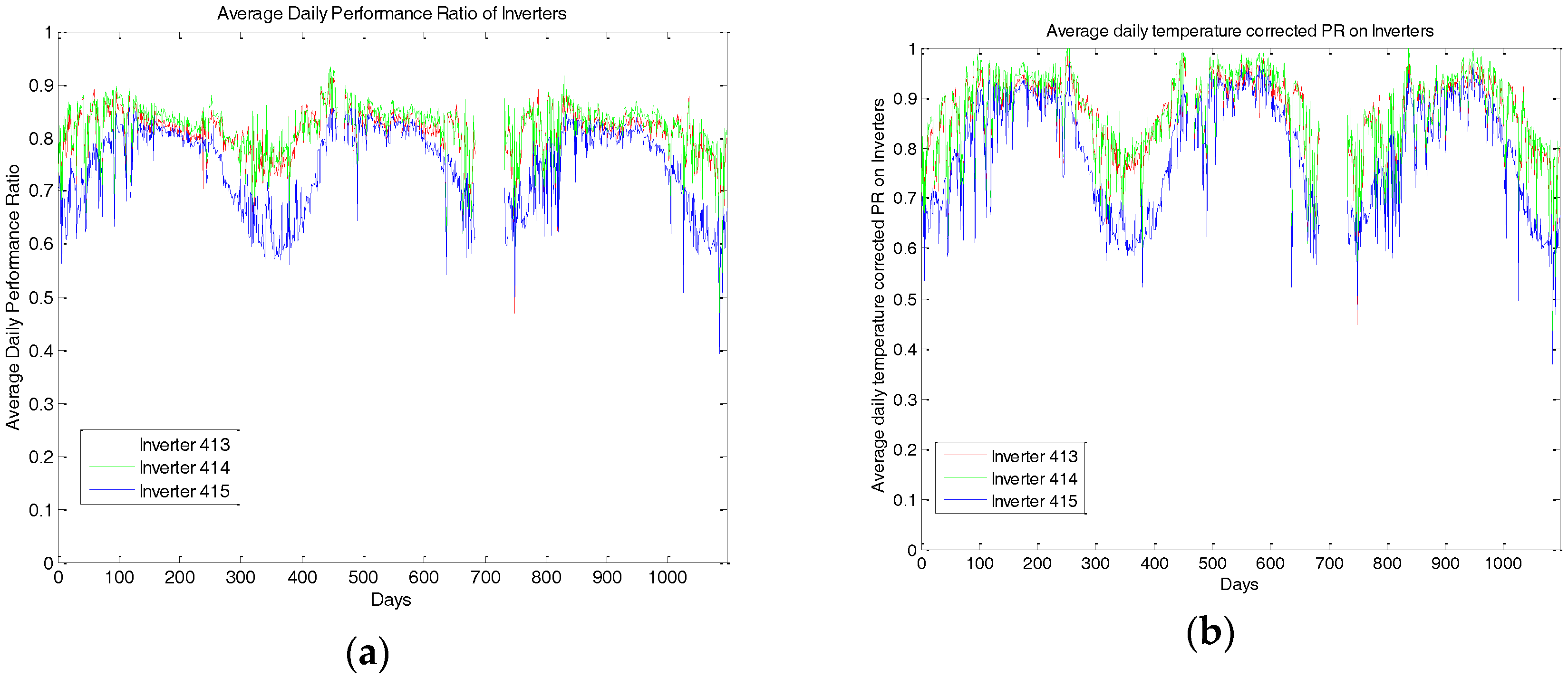
4.4. Performance Ratio

In Figure 9a, the PR value corresponding to the output in each of the three inverters is represented during the entire monitoring period. In Figure 9b an enlargement corresponding to values of inverter 413 is represented. In agreement with the aspects previously seen, it is observed that inverter 415 presents a smaller value of this parameter, and more significantly during the months of autumn and winter. From November to January, the value of PR in this inverter is lower than that of the other two throughout the day, while, during the months of September, October, February and March, these lower values are only concentrated in the first hours of the day. This behavior is repeated during the three years in which this installation is analyzed, which is showing, as already seen, the presence of shadows in the panels corresponding to this inverter during these months of the year, which do not affect the panels of the two remaining inverters or do so at very specific times of the day. This behavior is easily revealed thanks to the visualization of this parameter using color maps. On the other hand, the daily profiles corresponding to PR values are subject to irradiance and temperature conditions. When days are clear, without clouds, the daily profiles of this parameter, especially in inverters 413 and 414, present a behavior that is being repeated throughout the year. In the mornings, after the grid connection, when the inverter starts to generate electricity, the value of PR goes from a null value to a value close to 1 in a time of about one hour or even less. In the central hours of the day, the value of PR decreases, with a value between 0.8 and 0.9, depending on the time of year. This decrease could be due to the higher temperature losses that take place during this time and more significantly in the summer months. Subsequently, a new increase in the value of PR occurs, reaching from 18:00 the highest values of the day, even higher than 1 (red color in the figure), and then decreasing its value in the last moments of production. The shape of this curve is also observed by other authors, who call it a “bath tube” [12]. These authors indicate that the high temperature in the central hours of the day contributes to the reduction of the PR value.

In theory, the value of PR can be effectively higher than 1 because the panel nominal power is measured at STC, so it can be higher than 1 under more favorable conditions, such as higher irradiation or lower temperature than STC [12]. During the hours in which the PR values above 1 were obtained in this work, the irradiance did not present values superior to 1000 W/m² (Figure 3a). At these instants of time in the winter, the temperature of the module decreased below 25 °C. In summer, at these instants of time, the temperatures had already begun to fall, but they were still high, above 25 °C, and the PR peak with values greater than 1 occurred even with more incidence. This apparent increase in PR value could be influenced by a lack of synchronization in the data record, by a sub-estimation of the nominal power of the plant used for normalization, P_STC, or by an overestimation of the E_AC values recorded by a calibration error, although all these reasons would have the same effect during all the hours of the day and would not have a greater incidence at specific hours of the day. One might think this is due to an underestimation of the measured reference energy values, E_r, due to the presence of shading in the irradiance sensor, which did not affect the PV panels in the same way. There may also be affecting a different response of the PV panels, which are of polycrystalline silicon, compared to those of the reference cells used to record the irradiance, which is of amorphous silicon, since both materials have a different response to the spectrum of solar radiation [75].

The average daily values of PR are shown in Figure 10a. In this case, the PR values have been determined by only taking into account the instants of the monitoring period in which each inverter was available and producing electricity, not counting the instants in which there have been stops in the PV production. With the data of this figure, several conclusions can be obtained. First, the seasonality in the annual variation of these daily average values can be seen, mainly in the case of inverter 415. The months in which the PR values are higher correspond generally to the months of April and May. During these months, the values of irradiance have high values, but the higher temperatures that occur later during the summer months, which increase the losses in the capture system due to the temperatures, are not yet recorded. This is the reason the PR highest values do not take place in the summer. The highest PR values are those corresponding to inverter 414, being slightly lower, although with the same behavior throughout the year, those corresponding to inverter 413. The lower values correspond to inverter 415. The maximum values of the daily PR values found during the monitoring period were 0.92 (22 March 2012), 0.93 (22 March 2012) and 0.86 (27April 2011), corresponding to inverters 413, 414 and 415, respectively, being the minimum values 0.40%, 0.42% and 0.39%, all registered on 19 December 2013.

The values of the temperature-corrected performance ratio, TC_PR (Figure 10b), are higher than those of PR because the effects of temperature losses are removed. The maximum values were 0.98, 1.02 and 0.97 for inverters 413, 414 and 415, respectively, whereas the minimum values were 0.37, 0.39 and 0.37, respectively. It can be observed that the seasonal variation is not eliminated at all due to the presence of other factors that are causing seasonal variations, with a high impact in this PV installation, such as seasonally dependent shading and/or spectral effects.

To compare these results with those of other authors, it should be noted that the PR value has been determined with tilted irradiance instead of horizontal values. Moreover, it must be considered that, on an annual basis, crystalline silicon sensors measure less irradiation than pyranometers, although the difference between the two types of sensors depends very much on the sensor and the location (in Germany, the difference is around 2–4%). Therefore, the annual PR of a PV plant that is calculated on the basis of crystalline silicon sensors may be higher than PR based on pyranometer measurements [12,65,66]. In that regard, no information was found in the case of amorphous silicon sensors, which was the sensor used in this work.

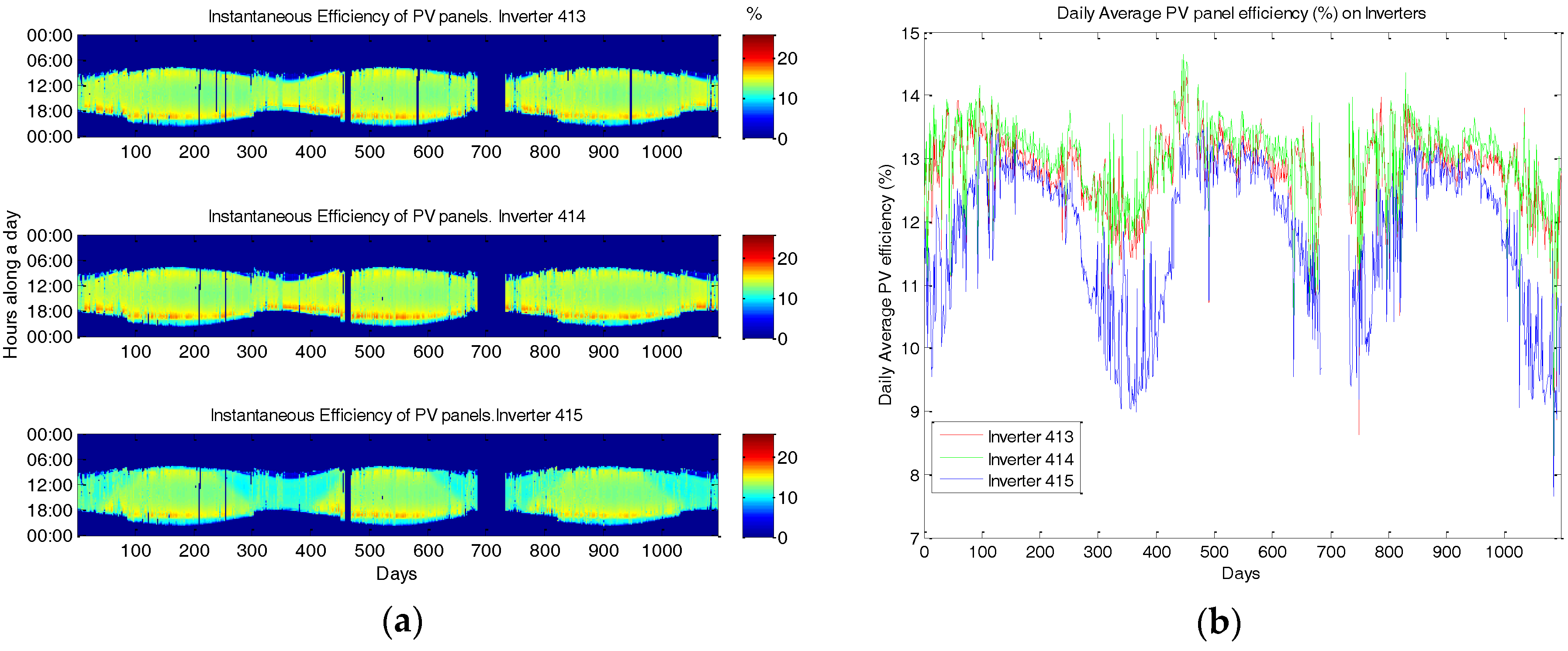
4.5. PV Panel Efficiency

In Figure 11a, the instantaneous values of the efficiency of the PV panels during the whole monitoring period are depicted. It is observed that the behavior presented by this parameter during the day was very similar to the one that has the PR of the production associated to each one of the inverters during the whole period of monitoring (Figure 9a). The values of the modules’ efficiency were slightly higher in the first and last hours of the day, with values higher than 15% and even 20% (which is a value above the 13.1% given by the manufacturer), while the value was lower in the central hours of the day, around 12–13% (depending on the time of year). The upper values in the first and last hours of the day also presented a certain periodicity such that these values were also slightly higher in the spring and summer months. If Figure 11b is observed, in which the average daily values of the efficiency of the panels are represented, the same behavior as that of the daily mean values of PR can be noticed. The lowest values are presented by inverter 415, mainly during the months from September to March. The maximum values of the average daily module efficiency were 14.36% (19 and 22 April 2012), 14.66% (22 March 2012) and 13.50% (27 April 2011 and 2 May 2012), respectively, for modules connected to inverters 413, 414 and 415, in the same range of values found by other authors for a near geographical location [76], being the minimum values 7.76%, 8.14% and 7.65% (19 December 2013).

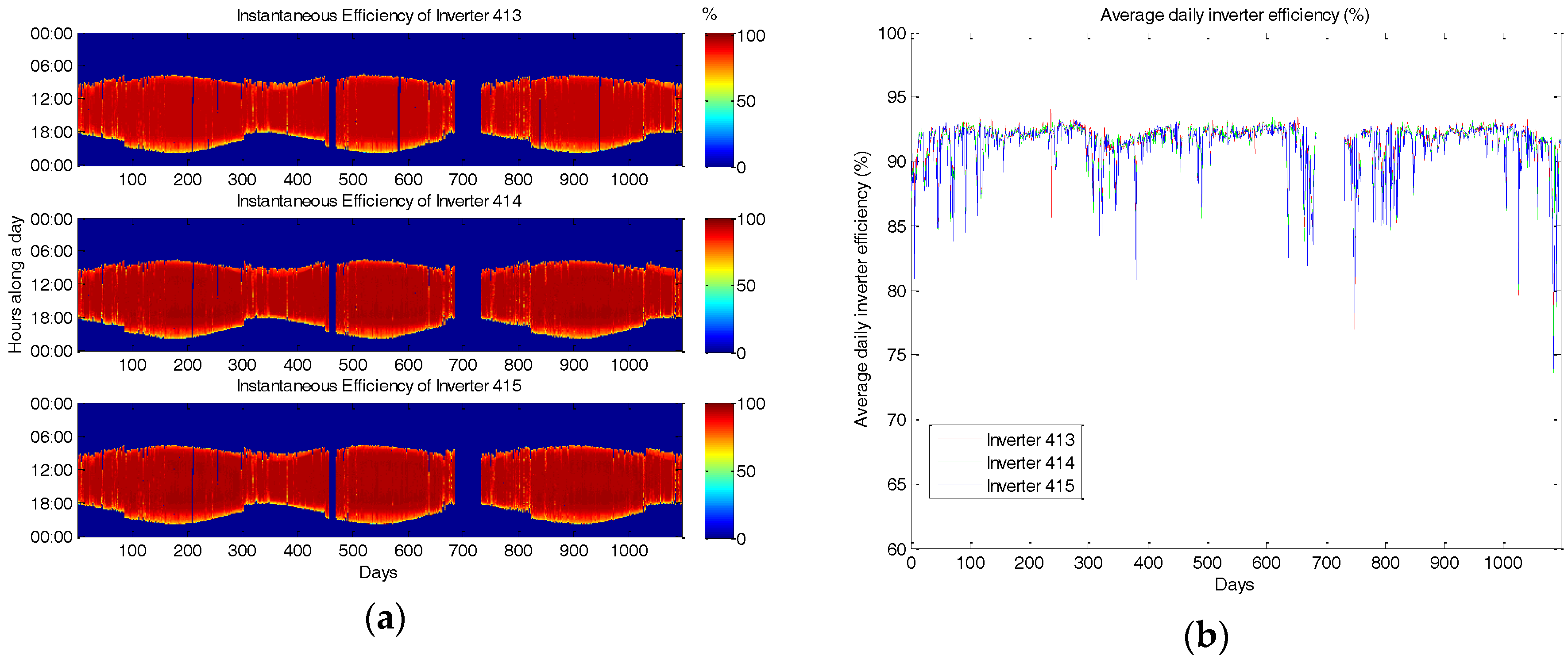
4.6. Inverter Efficiency

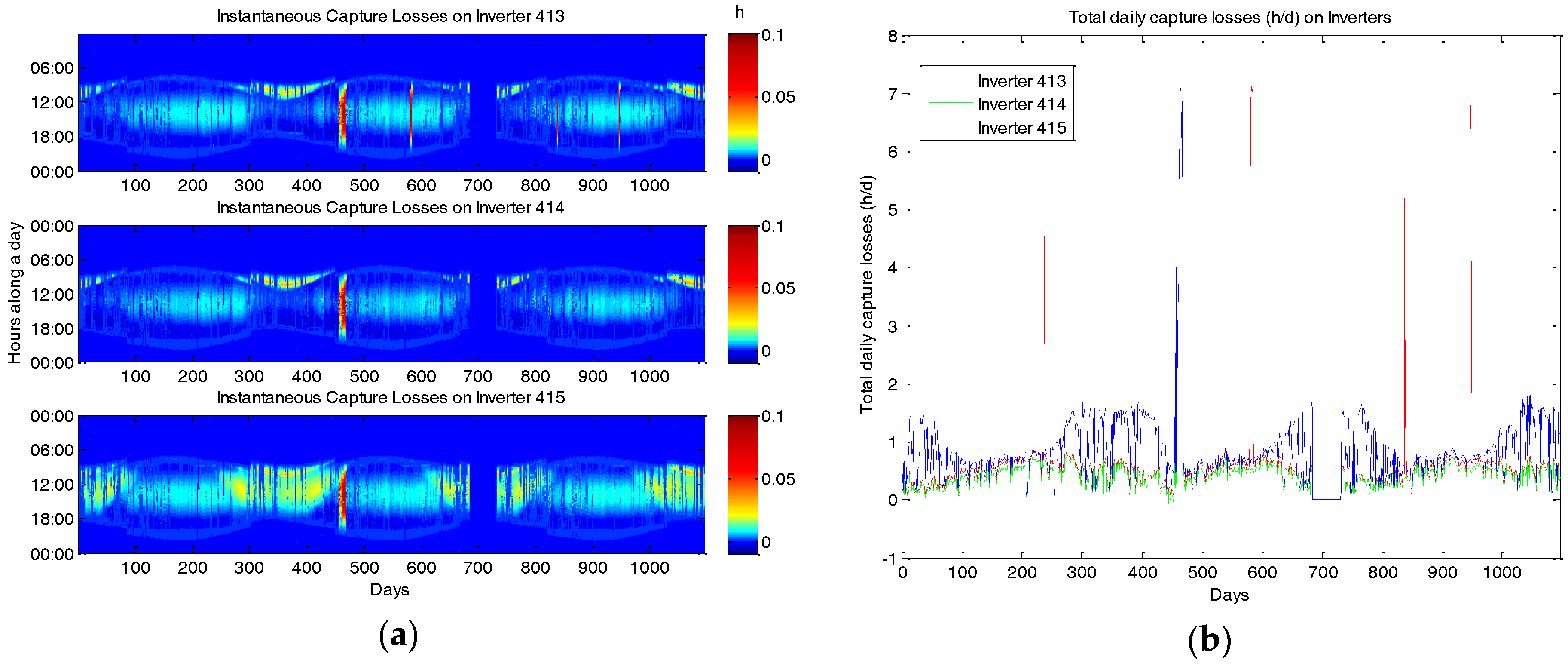
Figure 12a shows the instantaneous values of the efficiency of the three inverters, observing that, in this case, the profiles throughout the day were different from those presented by the efficiency of the panels. Although the efficiency was lower in the first and last hours of production, it rapidly increased to reach, during almost all the hours of production, values higher than 90%, which remained practically constant. In this case, the profiles and values found were very similar for the three inverters, as is also shown in Figure 12b, where it is observed that the average daily values of the inverters’ efficiency were practically the same in all three. The effect of the seasonality, although present, was lower in this parameter. These average values were above 90%, being slightly lower in the winter months and with greater variations from one day to another, between 75% and 92%. The highest values found were 94.00% (25 August 2011, Day 237), 93.37% (1 September 2012, Day 610) and 93.21% (6 October 2011, Day 279), respectively, for inverters 413, 414 and 415, being the minimum values equal to 75.02%, 73.57% and 73.92%, which took place on 19 December 2013 (Day 1084).

4.7. Capture Losses

Figure 13a shows at a glance the distribution of losses occurring in the capture systems connected to the three inverters throughout the whole monitored period. One the one hand, the losses occurring in the central hours of the day can be distinguished. They are mainly caused by temperature losses (which present the same daily profile and the same seasonality as the temperature values reflected in Figure 4a,b), which occurred with greater incidence in summer months and equally affect the panels of the three inverters. The wiring losses will be proportional to the production, so they will also be higher in the central hours of the day. On the other hand, the presence of losses that occur in the first and last hours of the day can be observed, which present a seasonal behavior, affecting to a greater extent the PV panels corresponding to inverter 415. These losses had a higher incidence in the months of autumn and winter, being higher the time interval in which inverter 415 is affected.

The losses by dirt and dust accumulated on the solar module surface, blocking some of the sunlight and reducing the output production, also affected the reference cell used to measure the radiation received by the panels [12]. Although dirt and dust are cleaned off during every rain event, it is necessary to clean them during dry periods. This type of intervention was not carried out in the installation, so this type of loss could not be evaluated. To do this, it is necessary to compare the performance, in situations where only the sensor is cleaned, with those in which both sensors and PV modules were cleaned [77].

Figure 13a also shows losses that occurred due to the presence of stops in production, already noticed in Figure 5a,b and Figure 6. On one occasion, this shutdown affected the three inverters, while it only affected inverter 413 on four other occasions.

In accordance with these results are those reflected in Figure 13b, in which the total daily values of capture losses are represented. For a typical day of July, total daily losses have been quantified at 0.72, 0.60 and 0.75 h/day for the arrays corresponding to the panels of inverters 413, 414 and 415, respectively, whereas, for a clear day in January, these losses may be 0.65, 0.60 and 1.63 h/day. It becomes clear that, although the temperature losses are higher in summer, they are more affected by shading losses in winter, influencing inverter 415 to a greater extent. The lowest losses were recorded in the months of April and May, the same ones in which the PR values were improved. This information can be taken into account when making stops at the facility for maintenance issues in order to carry them out in the periods of lower electricity production. It would be recommended that these two graphs be updated daily and monitored by O&M operators to quickly detect any deviations in production or abnormal operation.

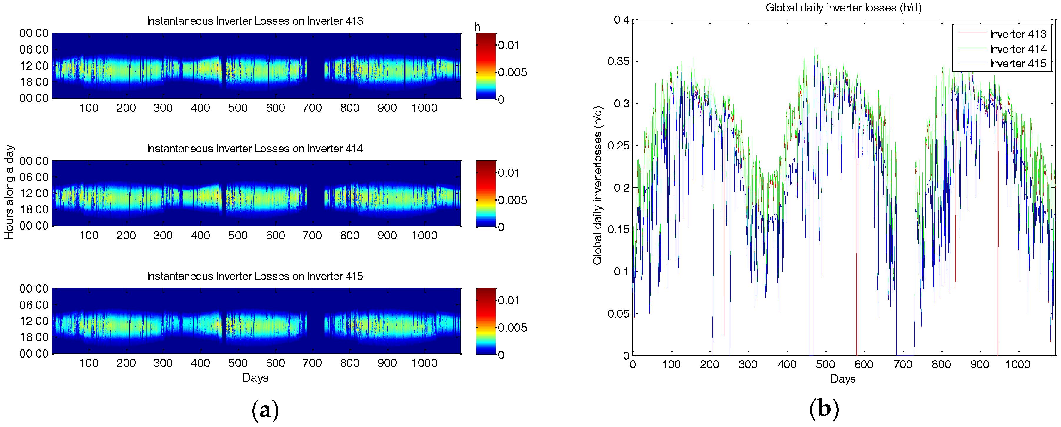
4.8. Inverter Losses

With respect to inverter losses, their instantaneous and daily total values are reflected in Figure 14a,b, respectively. As shown in Figure 14a, these losses were higher in the central hours of the day in which the production was higher. Since inverter 415 has a lower production in the autumn-winter months, it also has fewer losses during those months than the other two inverters, which is a fact that can be observed in both figures.

The daily total losses in the inverters were lower than those that take place in the PV modules, in line with the greater efficiency with which the inverters worked. The maximum values determined were 0.36, 0.36 and 0.35 h/day for inverters 413, 414 and 415, respectively, which took place on 16 April 2012 (Day 472). In general, although there were not any large variations in this type of losses from one day to the other throughout the year, the periods in which the highest losses in inverters were recorded were the months of April, May and June.

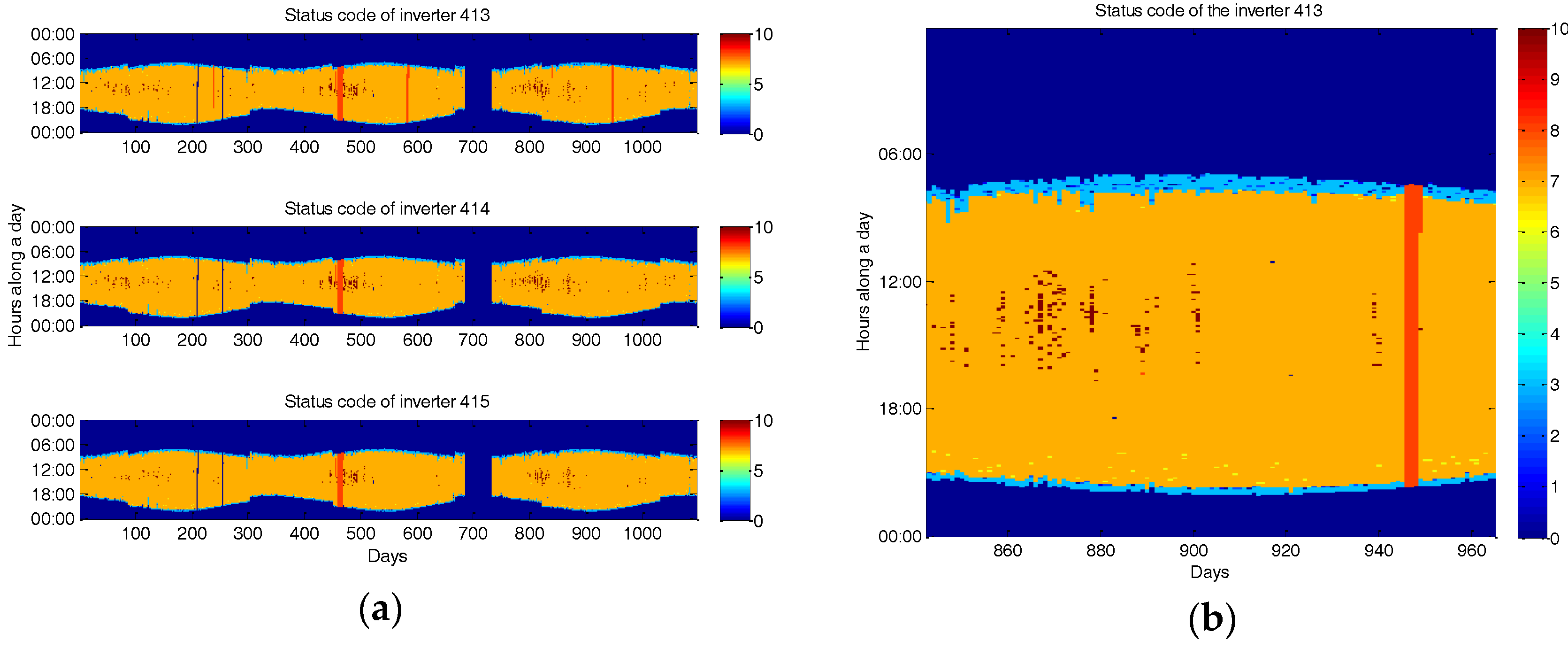
4.9. Inverter States

To analyze the behavior of inverters in Figure 15a their states have been represented during the entire monitoring period, and are codified with a series of numbers. An enlargement corresponding to inverter 413’s states is represented in Figure 15b.

When inverters are not working, the null value has been assigned (dark blue color). In the first and last hours of production, in which the inverter is in the start-up and shut-down phases, the inverters fundamentally monitored States 2 and 3 [13] (light blue color), which correspond, respectively, to a state in which inverters are monitoring the grid (which takes place just before connecting and disconnecting from the grid) and to a standby state, in which the requirements for the connection to the inverter to the grid are not yet fulfilled and the injection of current is waiting. Code 1 was also usually registered at start-up times, which is a state in which the inverter indicates an interruption after an error.

Once inverters are connected and in operation and are already injecting current into the grid, in the first few hours of operation or also in the later hours of the afternoon, the state that may be monitored was 6 (yellow color), in which the MPP (maximum power point) is being calculated. State 7 (orange color) is registered when the inverter is working in MPP. It was the most frequent state in which the inverters can be found. In it, the inverters ensure that the modules are in their optimum operating point for each external conditions, thus trying to extract the maximum power output of PV systems [39,78,79]. It can be observed that, except in the initial and final hours of the day, inverters were usually working in this state. Depending on the algorithm they use for the calculation, especially in the presence of shading, they will be getting more or less power from the PV array [80,81]. State 10 (brown color), named MPP peak, corresponds to that in which the inverter is operating in MPP mode, but above its rated capacity. This state occurred at the time of the year in which the higher values of irradiance were recorded, which took place in the months of February to June for the geographic location and the inclination and orientation of the PV panels, registering the highest values during the month of April. On clear days, inverters worked in this mode in the central hours of the day, around zenith. During these instants of time, inverters operated above their nominal power. The days of this period of the year with the passage of clouds cause the inverters to alternate their operation mode between MPP and MPP peak (compare Figure 15a and Figure 3a). For these instants in which inverters were worked in state 10 or MPP peak, the size of the PV array was overestimated, and the DC/AC inverter load ratio was higher than 1. State 10 appeared less frequently in inverter 415 than in the other two, since the output in the latter was lower. When inverters work above their nominal power, inverter heating increases. If this takes place for longer periods, its lifetime may be affected, so the cost of this type of degradation should be assessed against the initial savings that the underestimation of the inverter may involve.

On the other hand, State 8 (red color) corresponds to instants of time in which the inverter is recording information, but it is in a state of alert or warning, and it is not injecting electricity to the grid during those instants of time as a result of some kind of failure. The presence of this state in the graphs coincides with the instants in which there have been interruptions in the production, previously seen in the representation of both the energy generated in the PV arrays and in the representation of losses in the capture system. One or several daily supervisions of graphs such as the one presented in Figure 15 allow the O&M operators to quickly detect, simply by observing the color variations, deviations that would require an intervention in the plant.

5. Conclusions

The procedure proposed in this work has enabled us to effectively manage the large amount of data recorded in PV plants. The developed software accomplishes an automated migration of the registered data, the calculation of a series of performance and loss indexes of the components in the installation, and its storage in a RDBMS. Furthermore, it allows an easy and orderly access to the data the user is interested in. Specifically, the application provides the values of each parameter in the form of matrices, which have been represented in the form of color maps for their further study.

Even with the great amount of data generated, color maps enable representing each of these parameters during all the monitoring period in a readable way. This type of data visualization, with a broader scope than the daily or monthly values, provides a visual tool with which much information about the components’ behavior can be easily revealed in any instant of time. Its visual inspection enables one to detect the normal and abnormal modes of operation and to compare the behavior of the different components, helping in decision making related to O&M tasks. The analysis of these figures may serve to identify and interpret common design flows and operational problems or to simply document the operational mode of the installations in real conditions.

As a case study the operation of a grid-connected PV plant located in a city in southern Spain was studied using this type of graphs. All parameters were analyzed over a monitored period of three years to carry out a detailed study. With the color maps, it was possible to simultaneously represent the large volume data set obtained during the three years, and information about the behavior of panels and inverters was obtained. The average daily module efficiency values were in the range of 7.6–14.6%, whereas, for inverters, their average daily efficiency was in the range of 73.5–94%. It was possible to emphasize the presence of shadings in PV panels, with a greater impact on inverter 415. The hours and days of the year in which they take place were easily detected through this type of graphics. This has meant that for this inverter the daily values of PR range between 0.6 and 0.8, lower than the values of the other two inverters under normal operating conditions, between 0.7 and 0.9. The presence of stops or failures in the production was also easily detected by the visualization of the color maps corresponding to the loss indexes and to the inverter status.

Therefore, the developed application and this type of data visualization enable us to easily analyze the performance of PV systems and provide an affordable tool that may facilitate the corrective, preventive and predictive interventions of the O&M activities, generating information that can be considered in the design of future PV plants.

In addition to being easy to interpret, their use does not require an additional economic cost, since the data basically recorded by inverters were used. As it is indicated in the report of the International Energy Agency (IEA) [12], the inverter integrated measurements are usually not sufficiently precise and, in absolute terms, a more rigorous monitoring system would be necessary. Nevertheless, inverter data may be useful enough to know the behavior of the components of the PV installation and for identifying relative changes over time or deviations from their normal operation. However, it is important to know the limitations of this type of measure to correctly interpret the results. The use of an advanced monitoring system compared to the simple inverter monitoring depends very much on the individual project, and only if its use provides economic benefits will its implementation be justified.

The next objective is to apply the use of these graphs to the analysis of a megawatt PV park to manage the information corresponding to the monitoring of its components and to facilitate its maintenance, which will become the object of a future paper.

References

1. Schmela, M. Global Market Outlook for Solar Power 2017–2021. Available online: http://www.solarpowereurope.org/fileadmin/user_upload/documents/WEBINAR/Free_SolarPower_Webinar__Global_Market_Outlook_2017-2021.pdf (accessed on 24 November 2017).
2. Obi, M.; Bass, R. Trends and challenges of grid-connected photovoltaic systems—A review. Renew. Sustain. Energy Rev. 2016, 58, 1082–1094. [Google Scholar] [CrossRef]
3. Polman, A.; Knight, M.; Garnett, E.C.; Ehrler, B.; Sinke, W.C. Photovoltaic materials: Present efficiencies and future challenges. Science 2016, 352, aad4424. [Google Scholar] [CrossRef] [PubMed]
4. Bhakta, S.; Mukherjee, V. Solar potential assessment and performance indices analysis of photovoltaic generator for isolated Lakshadweep island of India. Sustain. Energy Technol. Assess. 2016, 17, 1–10. [Google Scholar] [CrossRef]
5. Nižetić, S.; Papadopoulos, A.M.; Giama, E. Comprehensive analysis and general economic-environmental evaluation of cooling techniques for photovoltaic panels, Part I: Passive cooling techniques. Energy Convers. Manag. 2017, 149, 334–354. [Google Scholar] [CrossRef]
6. Sampaio, P.G.V.; González, M.O.A. Photovoltaic solar energy: Conceptual framework. Renew. Sustain. Energy Rev. 2017, 74, 590–601. [Google Scholar] [CrossRef]
7. Utility-Scale Solar Photovoltaic Power Plants: A Project Developer’s Guide; International Finance Corporation: Washington, DC, USA, 2015.
8. Honrubia-Escribano, A.; Ramirez, F.J.; Gómez-Lázaro, E.; Garcia-Villaverde, P.M.; Ruiz-Ortega, M.J.; Parra-Requena, G. Influence of solar technology in the economic performance of PV power plants in Europe. A comprehensive analysis. Renew. Sustain. Energy Rev. 2018, 82, 488–501. [Google Scholar] [CrossRef]
9. Degener, S.; Watson, J. O&M Best Practices Guidelines. Available online: http://alectris.com/guidelines/om-best-practices-guidelines/ (accessed on 24 November 2017).
10. Moreno-Garcia, I.; Palacios-Garcia, E.; Pallares-Lopez, V.; Santiago, I.; Gonzalez-Redondo, M.; Varo-Martinez, M.; Real-Calvo, R. Real-time monitoring system for a utility-scale photovoltaic power plant. Sensors 2016, 16, 770. [Google Scholar] [CrossRef] [PubMed]
11. Rezk, H.; Tyukhov, I.; Al-Dhaifallah, M.; Tikhonov, A. Performance of data acquisition system for monitoring PV system parameters. Meas. J. Int. Meas. Confed. 2017, 104, 204–211. [Google Scholar] [CrossRef]
12. Woyte, A.; Ritcher, M.; Moser, D.; Reich, N.; Green, M.; Mau, S.; Garrad Hassan, G.; Beyer, H. Analytical Monitoring of Grid-Connected Photovoltaic Systems. Good Practices for Monitoring and Performance Analysis. 2014. Available online: http://iea-pvps.org/index.php?id=276 (accessed on 25 November 2017).
13. Haeberlin, H.; Beutler, C. Normalized representation of energy and power for analysis of performance and on-line error detection in PV-systems. In Proceedings of the 13th EU PV Conference on Photovoltaic Solar Energy Conversion, Nice, France, 23–27 October 1995. [Google Scholar]
14. Blaesser, G.; Munro, D. Guidelines for the Assessment of Photovoltaic Plants, Document A: Photovoltaic System Monitoring; Commission of the European Communities, Joint Research Centre: Ispra, Italy, 1995. [Google Scholar]
15. Blaesser, G.; Munro, D. Guidelines for the Assessment of Photovoltaic Plants, Document B: Analysis and Presentation of Monitoring Data; Commission of the European Communities, Joint Research Centre: Ispra, Italy, 1996. [Google Scholar]
16. International Standard IEC 61724: 1998 Photovoltaic System Performance Monitoring-Guidelines for Measurement, Data Exchange and Analysis. Edition 1.0; International Electrotechnical Commission: Geneva, Switzerland, 1998.
17. International Standard IEC 61724-1:2017 Photovoltaic System Performace-Part 1: Monitoring; International Electrotechnical Commission: Geneva, Switzerland, 2017.
18. Stefan, M.; Lopez, J.G.; Andreasen, M.H.; Olsen, R.L. Visualization Techniques for Electrical Grid Smart Metering Data: A Survey. In Proceedings of the 2017 IEEE Third International Conference on Big Data Computing Service and Applications (BigDataService), San Francisco, CA, USA, 6–9 April 2017; pp. 165–171. [Google Scholar] [CrossRef]
19. Moreno-Muñoz, A.; Flores-Arias, J.M.; Gil-De-Castro, A.; De La Rosa, J.J.G. Hypermedia user-interface integration in distribution power systems SCADA. In Proceedings of the 7th IEEE International Conference on Industrial Informatics (INDIN 2009), Cardiff, Wales, UK, 23–26 June 2009; pp. 136–141. [Google Scholar]
20. Murugesan, L.K.; Hoda, R.; Salcic, Z. Design criteria for visualization of energy consumption: A systematic literature review. Sustain. Cities Soc. 2015, 18, 1–12. [Google Scholar] [CrossRef]
21. Harrison, J.; Uhomobhi, J. Engineering study of tidal stream renewable energy generation and visualization: Issues of process modelling and implementation. In Lecture Notes in Computer Science (Including Subseries Lecture Notes in Artificial Intelligence and Lecture Notes in Bioinformatics); Springer International Publishing AG: Cham, Switzerland, 2016. [Google Scholar]
22. Filali-Yachou, S.; González-González, C.S.; Lecuona-Rebollo, C. HMI/ SCADA standards in the design of data center interfaces: A network operations center case study. DYNA 2015, 82, 180–186. [Google Scholar] [CrossRef]
23. US Department of Energy and NASPI. NASPI Synchrophasor Technical Report Phasor Tools Visualization Workshop Technical Summary; US Department of Energy and NASPI: Washington, DC, USA, 2014.
24. National Energy Technology Laboratory for the US Department of Energy. Office of Electricity Delivery and Energy Reliability Improved Interfaces and Decision Support; National Energy Technology Laboratory for the US Department of Energy: Pittsburgh, PA, USA, 2007.
25. Garoudja, E.; Harrou, F.; Sun, Y.; Kara, K.; Chouder, A.; Silvestre, S. Statistical fault detection in photovoltaic systems. Sol. Energy 2017, 150, 485–499. [Google Scholar] [CrossRef]
26. Ventura, C.; Tina, G.M. Utility scale photovoltaic plant indices and models for on-line monitoring and fault detection purposes. Electr. Power Syst. Res. 2016, 136, 43–56. [Google Scholar] [CrossRef]
27. Ventura, C.; Tina, G.M. Development of models for on-line diagnostic and energy assessment analysis of PV power plants: The study case of 1 MW Sicilian PV plant. Energy Procedia 2015, 83, 248–257. [Google Scholar] [CrossRef]
28. Chouder, A.; Silvestre, S. Automatic supervision and fault detection of PV systems based on power losses analysis. Energy Convers. Manag. 2010, 51, 1929–1937. [Google Scholar] [CrossRef]
29. Chouder, A.; Silvestre, S.; Taghezouit, B.; Karatepe, E. Monitoring, modelling and simulation of PV systems using LabVIEW. Sol. Energy 2013, 91, 337–349. [Google Scholar] [CrossRef]
30. Chouder, A.; Silvestre, S.; Sadaoui, N.; Rahmani, L. Modeling and simulation of a grid connected PV system based on the evaluation of main PV module parameters. Simul. Model. Pract. Theory 2012, 20, 46–58. [Google Scholar] [CrossRef]
31. Chine, W.; Mellit, A.; Pavan, A.M.; Kalogirou, S.A. Fault detection method for grid-connected photovoltaic plants. Renew. Energy 2014, 66, 99–110. [Google Scholar] [CrossRef]
32. de Lima, L.C.; de Araujo Ferreira, L.; de Lima Morais, F.H.B. Performance analysis of a grid connected photovoltaic system in northeastern Brazil. Energy Sustain. Dev. 2017, 37, 79–85. [Google Scholar] [CrossRef]
33. Malvoni, M.; Leggieri, A.; Maggiotto, G.; Congedo, P.M.; De Giorgi, M.G. Long term performance, losses and efficiency analysis of a 960 kW P photovoltaic system in the Mediterranean climate. Energy Convers. Manag. 2017, 145, 169–181. [Google Scholar] [CrossRef]
34. Ma, T.; Yang, H.; Lu, L. Long term performance analysis of a standalone photovoltaic system under real conditions. Appl. Energy 2016. [Google Scholar] [CrossRef]
35. Elhadj Sidi, C.E.B.; Ndiaye, M.L.; El Bah, M.; Mbodji, A.; Ndiaye, A.; Ndiaye, P.A. Performance analysis of the first large-scale (15 MWp) grid-connected photovoltaic plant in Mauritania. Energy Convers. Manag. 2016, 119, 411–421. [Google Scholar] [CrossRef]
36. Attari, K.; El Yaakoubi, A.; Asselman, A. Comparative Performance investigation between photovoltaic systems from two different cities. Procedia Eng. 2017, 181, 810–817. [Google Scholar] [CrossRef]
37. Attari, K.; Elyaakoubi, A.; Asselman, A. Performance analysis and investigation of a grid-connected photovoltaic installation in Morocco. Energy Rep. 2016, 2, 261–266. [Google Scholar] [CrossRef]
38. Bhakta, S.; Mukherjee, V. Performance indices evaluation and techno economic analysis of photovoltaic power plant for the application of isolated India’s island. Sustain. Energy Technol. Assess. 2017, 20, 9–24. [Google Scholar] [CrossRef]
39. Kumar, M.; Kumar, A. Performance assessment and degradation analysis of solar photovoltaic technologies: A review. Renew. Sustain. Energy Rev. 2017, 78, 554–587. [Google Scholar] [CrossRef]
40. Shiva Kumar, B.; Sudhakar, K. Performance evaluation of 10 MW grid connected solar photovoltaic power plant in India. Energy Rep. 2015, 1, 184–192. [Google Scholar] [CrossRef]
41. Sundaram, S.; Babu, J.S.C. Performance evaluation and validation of 5MWp grid connected solar photovoltaic plant in South India. Energy Convers. Manag. 2015, 100, 429–439. [Google Scholar] [CrossRef]
42. Micheli, D.; Alessandrini, S.; Radu, R.; Casula, I. Analysis of the outdoor performance and efficiency of two grid connected photovoltaic systems in northern Italy. Energy Convers. Manag. 2014, 80, 436–445. [Google Scholar] [CrossRef]
43. Padmavathi, K.; Daniel, S.A. Performance analysis of a 3MWp grid connected solar photovoltaic power plant in India. Energy Sustain. Dev. 2013, 17, 615–625. [Google Scholar] [CrossRef]
44. Wittkopf, S.; Valliappan, S.; Liu, L.; Ang, K.S.; Cheng, S.C.J. Analytical performance monitoring of a 142.5 kWp grid-connected rooftop BIPV system in Singapore. Renew. Energy 2012, 47, 9–20. [Google Scholar] [CrossRef]
45. Díez-Mediavilla, M.; Alonso-Tristán, C.; Rodríguez-Amigo, M.C.; García-Calderón, T.; Dieste-Velasco, M.I. Performance analysis of PV plants: Optimization for improving profitability. Energy Convers. Manag. 2012, 54, 17–23. [Google Scholar] [CrossRef]
46. Başoğlu, M.E.; Kazdaloğlu, A.; Erfidan, T.; Bilgin, M.Z.; Cąkir, B. Performance analyzes of different photovoltaic module technologies under İzmit, Kocaeli climatic conditions. Renew. Sustain. Energy Rev. 2015, 52, 357–365. [Google Scholar] [CrossRef]
47. Dabou, R.; Bouchafaa, F.; Arab, A.H.; Bouraiou, A.; Draou, M.D.; Neçaibia, A.; Mostefaoui, M. Monitoring and performance analysis of grid connected photovoltaic under different climatic conditions in south Algeria. Energy Convers. Manag. 2016, 130, 200–206. [Google Scholar] [CrossRef]
48. Shravanth Vasisht, M.; Srinivasan, J.; Ramasesha, S.K. Performance of solar photovoltaic installations: Effect of seasonal variations. Sol. Energy 2016, 131, 39–46. [Google Scholar] [CrossRef]
49. Edalati, S.; Ameri, M.; Iranmanesh, M. Comparative performance investigation of mono- and poly-crystalline silicon photovoltaic modules for use in grid-connected photovoltaic systems in dry climates. Appl. Energy 2015, 160, 255–265. [Google Scholar] [CrossRef]
50. Tripathi, B.; Yadav, P.; Rathod, S.; Kumar, M. Performance analysis and comparison of two silicon material based photovoltaic technologies under actual climatic conditions in Western India. Energy Convers. Manag. 2014, 80, 97–102. [Google Scholar] [CrossRef]
51. Milosavljević, D.D.; Pavlović, T.M.; Piršl, D.S. Performance analysis of A grid-connected solar PV plant in Nis, republic of Serbia. Renew. Sustain. Energy Rev. 2015, 44, 423–435. [Google Scholar] [CrossRef]
52. Congedo, P.M.; Malvoni, M.; Mele, M.; De Giorgi, M.G. Performance measurements of monocrystalline silicon PV modules in South-eastern Italy. Energy Convers. Manag. 2013, 68, 1–10. [Google Scholar] [CrossRef]
53. Drif, M.; Pérez, P.J.; Aguilera, J.; Almonacid, G.; Gomez, P.; de la Casa, J.; Aguilar, J.D. Univer Project. A grid connected photovoltaic system of 200 kWp at Jaen University. Overview and performance analysis. Sol. Energy Mater. Sol. Cells 2007, 91, 670–683. [Google Scholar] [CrossRef]
54. Trillo-Montero, D.; Santiago, I.; Luna-Rodriguez, J.J.; Real-Calvo, R. Development of a software application to evaluate the performance and energy losses of grid-connected photovoltaic systems. Energy Convers. Manag. 2014, 81. [Google Scholar] [CrossRef]
55. Fernández-Pacheco, D.G.; Molina-Martínez, J.M.; Ruiz-Canales, A.; Jiménez, M. A new mobile application for maintenance tasks in photovoltaic installations by using GPS data. Energy Convers. Manag. 2012, 57, 79–85. [Google Scholar] [CrossRef]
56. Silvestre, S.; Chouder, A.; Karatepe, E. Automatic fault detection in grid connected PV systems. Sol. Energy 2013, 94, 119–127. [Google Scholar] [CrossRef]
57. Gokmen, N.; Karatepe, E.; Silvestre, S.; Celik, B.; Ortega, P. An efficient fault diagnosis method for PV systems based on operating voltage-window. Energy Convers. Manag. 2013, 73, 350–360. [Google Scholar] [CrossRef]
58. Kymakis, E.; Kalykakis, S.; Papazoglou, T.M. Performance analysis of a grid connected photovoltaic park on the island of Crete. Energy Convers. Manag. 2009, 50, 433–438. [Google Scholar] [CrossRef]
59. Al-Sabounchi, A.M.; Yalyali, S.A.; Al-Thani, H.A. Design and performance evaluation of a photovoltaic grid-connected system in hot weather conditions. Renew. Energy 2013, 53, 71–78. [Google Scholar] [CrossRef]
60. Koehl, M.; Heck, M.; Wiesmeier, S.; Wirth, J. Modeling of the nominal operating cell temperature based on outdoor weathering. Sol. Energy Mater. Sol. Cells 2011, 95, 1638–1646. [Google Scholar] [CrossRef]
61. Skoplaki, E.; Boudouvis, A.G.; Palyvos, J.A. A simple correlation for the operating temperature of photovoltaic modules of arbitrary mounting. Sol. Energy Mater. Sol. Cells 2008, 92, 1393–1402. [Google Scholar] [CrossRef]
62. Skoplaki, E.; Palyvos, J.A. Operating temperature of photovoltaic modules: A survey of pertinent correlations. Renew. Energy 2009, 34, 23–29. [Google Scholar] [CrossRef]
63. Fuentes, M. A Simplified Thermal Model for Flat-Plate Photovoltaic Arrays; Report SAND-85-0330; United States Department of Commerce: Washington, DC, USA, 1987.
64. Chatzipanagi, A.; Frontini, F.; Dittmann, S. Investigation of the influence of module working temperatures on the performance of BiPV modules. In Proceedings of the 27th European Photovoltaic Solar Energy Conference and Exhibition, Frankfurt, Germany, 24–28 September 2012; pp. 4192–4197. [Google Scholar]
65. Reich, N.H.; Mueller, B.; Armbruster, A.; Van Sark, W.G.J.H.M.; Kiefer, K.; Reise, C. Performance ratio revisited: Is PR > 90% realistic? Prog. Photovolt. Res. Appl. 2012, 20, 717–726. [Google Scholar] [CrossRef]
66. Khalid, A.M.; Mitra, I.; Warmuth, W.; Schacht, V. Performance ratio—Crucial parameter for grid connected PV plants. Renew. Sustain. Energy Rev. 2016, 65, 1139–1158. [Google Scholar] [CrossRef]
67. Perpiñan, O. Energía Solar Fotovoltaica; Creative Commons: Boston, MA, USA, 2012. [Google Scholar]
68. Phyton. Available online: https://www.python.org/ (accessed on 1 October 2017).
69. HTML. Available online: https://www.w3schools.com/html/ (accessed on 1 October 2017).
70. CSS. Available online: https://www.w3schools.com/css/default.asp (accessed on 1 October 2017).
71. TypeScript. Available online: https://www.typescriptlang.org/ (accessed on 1 October 2017).
72. Solar del Valle, SL Company. Available online: http://www.solardelvalle.es (accessed on 17 November 2017).
73. SMA Company. Available online: https://www.sma.de/en.html (accessed on 17 November 2017).
74. Gobierno de España Real Decreto 1578/2008, de 26 de septiembre, de retribución de la actividad de producción de energía eléctrica mediante tecnología solar fotovoltaica para instalaciones posteriores a la fecha límite de mantenimiento de la retribución del Real Decreto 661/2008. Boletín Ofical del Estado 2008, 234, 39117–39125.
75. Chegaar, M.; Mialhe, P. Effect of atmospheric parameters on the silicon solar cells performance. J. Electron Devices 2008, 6, 173–176. [Google Scholar]
76. Cañete, C.; Carretero, J.; Sidrach-de-Cardona, M. Energy performance of different photovoltaic module technologies under outdoor conditions. Energy 2014, 65, 295–302. [Google Scholar] [CrossRef]
77. Touati, F.; Al-Hitmi, M.A.; Chowdhury, N.A.; Hamad, J.A.; San Pedro Gonzales, A.J.R. Investigation of solar PV performance under Doha weather using a customized measurement and monitoring system. Renew. Energy 2016, 89, 564–577. [Google Scholar] [CrossRef]
78. Lupangu, C.; Bansal, R.C. A review of technical issues on the development of solar photovoltaic systems. Renew. Sustain. Energy Rev. 2017, 73, 950–965. [Google Scholar] [CrossRef]
79. Rezk, H.; Fathy, A.; Abdelaziz, A.Y. A comparison of different global MPPT techniques based on meta-heuristic algorithms for photovoltaic system subjected to partial shading conditions. Renew. Sustain. Energy Rev. 2017, 74, 377–386. [Google Scholar] [CrossRef]
80. Ram, J.P.; Babu, T.S.; Rajasekar, N. A comprehensive review on solar PV maximum power point tracking techniques. Renew. Sustain. Energy Rev. 2017, 67, 826–847. [Google Scholar] [CrossRef]
81. Dileep, G.; Singh, S.N. Application of soft computing techniques for maximum power point tracking of SPV system. Sol. Energy 2017, 141, 182–202. [Google Scholar] [CrossRef]
Figure 1. Esquematic diagram of the procedure used by S·lar2 for the automated processing of monitored data in PV installations.
Energies 10 01964 g001
Figure 2. S·lar2’s graphical user interface (GUI): (a) selection of data; and (b) graphical visualization of selected parameter (EDC) for the three inverters.
Energies 10 01964 g002
Figure 3. Tilted irradiance registered from 1 January 2011 to 31 December 2013: (a) instantaneous values, during 24 h a day; and (b) total daily values.
Energies 10 01964 g003
Figure 4. Registered ambient and module temperature, and calculated cell temperature registered from 1 January 2011 to 31 December 2013: (a) instantaneous values, during 24 h a day; and (b) average daily values.
Energies 10 01964 g004
Figure 5. Instantaneous DC energy generated in the PV arrays connected to inverters registered from 1 January 2011 to 31 December 2013: (a) instantaneous values, during 24 h a day; and (b) total daily values.
Energies 10 01964 g005
Figure 6. Total daily DC energy generated in the PV arrays connected to inverters, from 23 June 2012 to 15 September 2012.
Energies 10 01964 g006
Figure 7. Inverters that are producing the maximum amount of energy EAC in each instant of time from 1 January 2011 to 31 December 2013.
Energies 10 01964 g007
Figure 8. Instantaneous differences, in percentage of nominal power, of the production of each inverter with regard to that of the maximum production, in each instant of time: (a) from 1 January 2011 to 31 December 2013; and (b) on 25 February 2011 and on 17 June 2011.
Energies 10 01964 g008
Figure 9. (a) Instantaneous values of performance ratio of the three inverters, during 24 h a day, from 1 January 2011 to 31 December 2013; and (b) enlargement of performance ratio values of inverter 413.
Energies 10 01964 g009
Figure 10. (a) Average daily performance ratio; and (b) average daily corrected temperature performance ratio of the production of the three inverters, from 1 January 2011 to 31 December 2013
Energies 10 01964 g010
Figure 11. PV panels’ efficiency from 1 January 2011 to 31 December 2013: (a) instantaneous values, during 24 h a day; and (b) total daily values.
Energies 10 01964 g011
Figure 12. Inverters’ efficiency from 1 January 2011 to 31 December 2013: (a) instantaneous values, during 24 h a day; and (b) total daily values.
Energies 10 01964 g012
Figure 13. Capture losses from 1 January 2011 to 31 December 2013: (a) instantaneous values, during 24 h a day; and (b) total daily values.
Energies 10 01964 g013
Figure 14. Inverter losses, from 1 January 2011 to 31 December 2013: (a) instantaneous values, during 24 h a day; and (b) total daily values.
Energies 10 01964 g014
Figure 15. (a) instantaneous values of performance ratio of the three inverters, during 24 h a day, from 1 January 2011 to 31 December 2013: and (b) enlargement of status values of inverter 413.
Energies 10 01964 g015