A New Control-Oriented Semi-Empirical Approach to Predict Engine-Out NOx Emissions in a Euro VI 3.0 L Diesel Engine


1
Department of Energy, Politecnico di Torino, Corso Duca degli Abruzzi 24, 10129 Torino, Italy
2
FPT Motorenforschung AG, Schlossgasse 2, 9320 Arbon, Switzerland
*
Author to whom correspondence should be addressed.
Energies 2017, 10(12), 1978; https://doi.org/10.3390/en10121978
Submission received: 31 October 2017
/
Revised: 23 November 2017
/
Accepted: 26 November 2017
/
Published: 29 November 2017
(This article belongs to the Section I: Energy Fundamentals and Conversion)
Abstract
:The present study is focused on the development of a new control-oriented semi-empirical model to predict nitrogen oxide (NOx) emissions in a light-duty diesel engine under both steady-state and transient conditions. The model is based on the estimation of the deviations of NOx emissions, with respect to the nominal engine-calibration map values, as a function of the deviations of the intake oxygen concentration and of the combustion phasing. The model also takes into account the effects of engine speed, total injected quantity, and ambient temperature and humidity. The approach has been developed and assessed on an Fiat Powertrain Technologies (FPT) Euro VI 3.0 L diesel engine for light-duty applications, in the frame of a research project in collaboration with FPT Industrial. The model has also been tested on a rapid prototyping device, and it was shown that it requires a very short computational time, thus being suitable for implementation on the Engine Control Unit (ECU) for real-time NOx control tasks.
1. Introduction
NOx emission control constitutes a critical issue in modern diesel engines, considering the more and more stringent emission regulations. Future regulations in Europe will likely include the use of Portable Emissions Measurement Systems (PEMS), capable of monitoring pollutant emissions in real-time during vehicle operation [1].
Several techniques have been investigated to control NOx emissions from diesel vehicles, which include the use of more and more efficient after-treatment devices, such as, Lean NOx Traps (LNTs) or Selective Catalytic Reduction (SCR) devices [2], as well as the limitation of in-cylinder NOx formation.
With reference to the latter technique, innovative combustion modes have recently been explored, such as the Premixed Charge Compression Ignition (PCCI) mode or the Homogeneous Charge Compression Ignition (HCCI) mode. These combustion modes exploit a low-temperature highly-premixed combustion, and have the potential of reducing NOx and soot emissions at the same time [3]. However, these techniques are not yet fully adopted in commercial vehicles, and additional research efforts are still needed in order to fully exploit their potential.
In-cylinder NOx formation is instead typically controlled by means of Exhaust Gas Recirculation (EGR), of the internal or external type, and/or by means of a proper calibration of the injection parameters [4]. However, these techniques are typically calibrated at steady-state operation, and may be less effective in transient conditions, or at least require a high calibration effort in order to identify proper correction maps.
For this reason, interest in the development of NOx control techniques has increased in the last years, with specific focus on the transient operation. In general, control algorithms include closed-loop approaches, model-based techniques, or a combination of the two previous methods. Closed-loop algorithms require the installation of a NOx sensors at the engine exhaust [5]. However, NOx sensor measurements suffer from a slow response time [6,7], so that a fully closed-loop approach would not be effective to control NOx emissions in transient operation. A model-based approach, instead, has the potential of overcoming this issue. Interest in the development of model-based control algorithms has therefore increased recently, also due to the fact that the computational performance of Engine Control Units (ECUs) has increased in the last years [8,9].
Model-based control algorithms offer several advantages over the traditional map-based approaches. First, they require a lower experimental effort for calibration. Secondly, they offer the possibility of optimizing the engine calibration parameters in real-time, in order to achieve desired targets of performance or emission metrics which may be variable over time, depending on the state of other systems (such as, after-treatment devices) [8].
A model-based controller requires a fast and accurate approach to predict NOx emissions. In general, the simulation of NOx emissions can be performed using models characterized by different degrees of detail, such as phenomenological models, semi-empirical or empirical models, and black-box models.
Phenomenological approaches are generally based on a detailed modeling of the NOx formation process, starting from the knowledge of the in-cylinder thermodynamic and chemical properties of the charge. The latter properties can be obtained using CFD models, quasi-dimensional models or zero-dimensional models. Some examples of phenomenological NOx models are reported in [10,11,12,13,14,15,16,17,18,19].
In [10], a multizone model of combustion diagnostics was proposed to estimate heat release and NOx concentration. In [11] the authors developed a conversion of the previously developed diagnostic model into a predictive model, using physically-based models for fuel injection, ignition delay, premixed and diffusive heat release rate, and using tables with chemical equilibrium data. In [12,13], the authors proposed a NOx model based on the Zeldovich mechanism, in which the in-cylinder thermodynamic conditions were obtained through a real-time 3-zone model. In [14], an extended NO and soot production model was developed for both conventional and advanced, high-EGR heavy-duty DI diesel combustion. In [15], two NOx models coupled to a multizone quasi-dimensional phenomenological engine model were proposed in a direct-injection naturally aspirated diesel engine. In [16], a physics-based model for the NOx emissions, that required the in-cylinder pressure measurement, was developed and validated using data from three different engines. In [17], the previously developed NOx model was coupled to a mean-value model for the air path. In [18,19], NOx emissions were calculated by coupling predictive schemes to 3D-CFD combustion models.
Phenomenological approaches can lead to very accurate results, but they generally require a calculation time that is not suitable for real-time NOx control tasks, even considering the high performance of modern ECUs.
Empirical models, instead, are generally constituted by simplified correlations which rely on input data that can be measured directly. They require a much lower effort than phenomenological models in terms of computational time, but lack of physical consistency [20]. Semi-empirical models are similar to empirical models, but they usually include parameters which cannot be measured directly, and are more closely related to the NOx formation process, such as the maximum temperature of the burned gases during the combustion of the main pulse [20], the adiabatic flame temperature [21], the heat release rate [22,23]. In [24], a zero-dimensional NO model, which required a low calibration effort, was developed. In [25], the authors propose a method which is capable of estimating NOx emissions cycle-by-cycle, on the basis of the in-cylinder pressure, the air mass flow and the relative air-to-fuel ratio ‘lambda’. Semi-empirical models generally require a higher computational time than empirical models (this time depends on the sub-models that are adopted to estimate the non-measurable input variables), but they are physically-based and therefore they guarantee a higher level of accuracy. However, the computational time required by semi-empirical models is much smaller than that of phenomenological models, so that they are good candidates for real-time control tasks.
Finally, artificial intelligence systems and machine-learning techniques, such as artificial neural networks, have also been introduced in the literature as fast predictive tools for emissions [26,27]. These methods do not require the detailed knowledge of the physics of the system, since they are of the black-box or grey-box type. Moreover they require a very small computational time to be run, so that they are good candidates for the development of model-based control algorithms. They do, however, lack of physical consistency, and require a training that needs a high number of experimental tests in order to avoid overfitting and be sufficiently predictive [9]. Moreover, their performance is usually not reliable outside the calibration range.
Contribution of the Present Study
Given the previously reported background, semi-empirical correlations have been identified as the best candidates for control-oriented applications. A semi-empirical NOx model oriented to control applications has already been developed by the authors in [20] and refined in [8]. In that case, the model included, among the input parameters, the maximum temperature of the burned gases related to the main injection (i.e., Tbmax,main), the charge-to-fuel ratio, the injection pressure, the engine speed and the injected fuel mass. The evaluation of the temperature of the burned gases required the adoption of zero-dimensional predictive combustion model. Although the approach presented in [8,20] has been designed in order to have a low-throughput, it still requires a calculation time that is about 1.5 ms [8] when it is run on a rapid prototyping device, such as an ETAS ES910. The latter device is characterized by a computational performance which is 3–4 times faster than that of a modern ECU.
A NOx control algorithms needs to be run at a high frequency rate in order to guarantee a cycle-by-cycle control. Therefore, the approach proposed in [8] may not be currently suitable for onboard implementation, and an even stricter demand in terms of computational time may be required. Moreover, the model proposed in [8] is highly physically consistent, but also quite sensitive to an error in the input variables. In particular, it requires, among the variables, the air mass and the EGR mass, which have a great impact on the calculation of the in-cylinder burned gas temperatures and, therefore, on the NOx prediction accuracy. According to [23], a 5% error in the trapped mass estimation can lead to an error in the estimated NOx emissions that is around 100%.
Therefore, the aim of the present paper is the development and assessment of a new semi-empirical model to predict NOx emissions, which is sufficiently robust to input variable variance, but also very fast in order to be run on a modern ECU within high-frequency control tasks.
The model that has been proposed in this study is characterized by the following specifications:
- It is based on MFB50 (crank angle at which 50% of fuel-mass is burned), O2 (intake O2 concentration), N (engine speed) and qf,inj (total injected fuel quantity). In particular, it was found that MFB50 is a very robust metric that correlates well with the NOx formation. It will be shown that the MFB50 metric is able to account for the effects of injection timing and injection pressure simultaneously.
- The model has not been designed in order to predict the absolute values of NOx emissions, but is based on the prediction of the deviations of NOx emissions, with respect the nominal engine-map calibration values, as a function of the deviations of MFB50 and intake O2 concentration. This leads to several advantages. First, the variation range of the NOx deviations is much smaller than the variation range of the NOx absolute values. As a consequence, their prediction is more accurate, considering the high non-linearity of the NOx formation process. Second, the error of the model tends to zero when the deviations of the input parameters tend to zero, since the nominal NOx levels over the engine map are taken in this case.
- Finally, it was demonstrated that the proposed method is physically consistent, since it maintains a high accuracy even when the number of points used for calibration is very low, and that it requires a much smaller computational time than the previous model proposed in [8].
2. Experimental Setup and Engine Conditions
The experimental tests were measured for a FPT F1C 3.0 L Euro VI diesel engine. The main engine specifications are reported in Table 1.
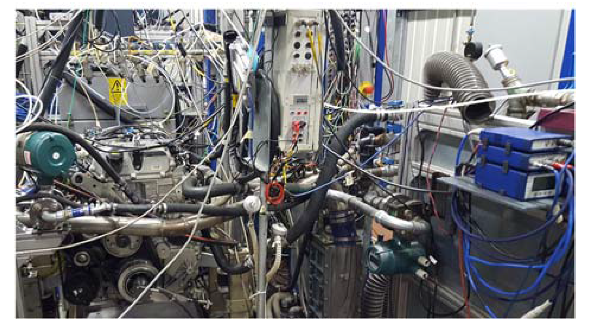
The engine is shown in Figure 1. A short-route EGR system equipped with a cooler is installed on the engine. The EGR valve is installed upstream from the EGR cooler. A flap is present in the exhaust pipe downstream the turbine, in order to control the temperature of the exhaust gas flowing to the after-treatment system and to increase EGR rate if necessary.
Figure 2 shows a scheme of the test bench (Figure 2a) and of the engine with the related sensors (Figure 2b). The test engine was instrumented with PT100 thermocouples and piezoresistive pressure transducers in order to acquire temperature and the pressure at several locations, such as upstream and downstream from the from the turbine (pT1, TT1, pT2, TT2), compressor (pC1, TC1, pC2, TC2), and intercooler (pIC1, TIC1, pIC2, TIC2), in the intake manifold (pint, Tint) and in the EGR circuit (TEGR1, TEGR2, pEC2, TEC2). The temperature was also acquired in each intake (Ti1, Ti2, Ti3, Ti4) and exhaust runner (Te1, Te2, Te3, Te4) by means of thermocouples.
Four 6058A high-frequency piezoelectric transducers (pcyl1, pcyl2, pcyl3, pcyl4) manufactured by Kistler (Winterthur, Switzerland) are placed in glow-plug adapters to acquire for each cylinder, on a crank basis, the in-cylinder pressure time-histories. The in-cylinder pressure traces are pegged on the basis of the intake pressure that is measured by means of a high-frequency Kistler 4007C piezo-resistive transducer, located in front of cylinder 1 (pi1,hf). On the exhaust side, a high-frequency cooled Kistler 4049B piezo-resistive transducers is also installed (pe1,hf).
The tests were carried out on the dynamic test rig at the Internal Combustion Engines Advanced Laboratory at the Politecnico di Torino (ICEAL-PT). The test bench is equipped with an ELIN APA 100 AC dynamometer manufactured by AVL (Graz, Austria) and an AVL KMA 4000 fuel meter. The latter is characterized by an accuracy of 0.1% over a 0.28–110 kg/h range. The raw engine-out gaseous emissions are measured by means of an AVL AMAi60- endowed with two complete trains equipped with devices for the simultaneous measurement of gaseous concentrations of HC, CH4, NOx/NO, CO, CO2 and O2 both at the intake and exhaust manifolds. Finally, for the soot measurement an ‘AVL 415S’ smokemeter is used for steady-state tests whereas an AVL 439 opacimeter is adopted for transient tests. The measurement devices were controlled by the AVL PUMA OPEN 1.3.2 automation system.
An ES910 rapid prototyping device manufactured by ETAS (Stuttgart, Germany) was used to realize pressure-based and model-based controls of the combustion phasing on the engine (see [30]), and to test the real-time capability of the proposed NOx model. The main specifications of the ETAS ES910 device are shown in Table 2.
Experimental Activity
The experimental tests that have been used in the present study include steady-state tests and transient tests. The following tests were considered (Figure 3):
- A full engine map including 123 points.
- EGR-sweep tests at fixed key-points, including 162 points. EGR rate was varied from 0 to 50% by setting different levels of trapped air mass with steps of 50 mg/cycle.
- Sweep tests of main injection timing (SOImain) and injection pressure (pf) at fixed key-points, including 125 points. A SOImain variation of ±6 crank angle degrees around the nominal values and a pf variation of ±20% around the nominal values were set. A pilot-main injection strategy was adopted, in which the pilot quantity and the dwell-time between the pilot and main pulses was kept constant. The tests were carried out in “BMEP-control” mode. This means that, during the tests, the software of the test bench acted on the total injected quantity in order to maintain a constant value of BMEP corresponding to the desired target.
The developed NOx model was tested on the engine over different load/speed ramps. Details on these ramps are reported in the Results and Discussion section.
With reference to the fuel used in the present investigation, the engine was fed with conventional diesel fuel (according to EN 590 regulations), whose main properties are listed in Table 3.
3. Model Description
After a general discussion about the NOx formation process and some recalls on the previous semi-empirical NOx model proposed by the authors in [8] (Section 3.1), the identification of the input variables of the proposed NOx model is described in Section 3.2, while the NOx model is presented in Section 3.3. Section 3.4 reports a quick summary on the predictive combustion model that is necessary to adopt when using the previous semi-empirical NOx model described in [8]. Some considerations concerning the model recalibration when applied to different engines are finally reported in Section 3.5.
3.1. NOx Formation Process and Recalls on the previously developed NOx Model
The acronym ‘‘NOx’’ is generally intended as the sum of NO (nitrogen monoxide) and NO2 (nitrogen dioxide) emissions [20]. NO2 emissions in diesel engines are generally around 10–30% of the total NOx emissions, especially at lower load conditions [31,32]. However, in the literature, only the NO emissions are generally modeled, and the values of predicted NO values are taken as representative of the total NOx emission levels [20]. The NO formation process mainly depends on several mechanisms: the thermal mechanism, which is temperature-dependent, the prompt mechanism [33] and the fuel-derived NO mechanism [20].
The thermal NO formation was described by the extended Zeldovich mechanism [34,35], which was refined according to the super-extended Zeldovich mechanism [36]. The Zeldovich mechanism is enhanced by the high local temperatures of the gases, which cause O2 dissociation, and by the quantity of O2 in the burning region. In general, the thermal mechanism leads to the predominant NOx formation contribution.
The semi-empirical approach previously proposed by the authors in [20] was based on several variables, which were identified starting from the analysis of the NOx formation rate according to the Zeldovich mechanism. These variables are the maximum temperature of the burned gases during the combustion of the main pulse ‘Tbmax,main’, the total mass of injected fuel (mfuel) (or, analogously, the total injected fuel volume quantity, ‘qf,inj’), the engine speed ‘N’, the injection pressure ‘pf’ and the stoichiometric in-cylinder charge-to-fuel ratio ‘’. The NOx model reported in [20] needs to be coupled with a predictive combustion model, in order to estimate the temperature of the burned gases.
The approach proposed in [20] was subsequently revised in [8]: the ‘Tbmax,main’ was replaced by the ‘Tb,MFB50’ term (i.e., the burned gas temperature evaluated at MFB50). The ‘Tb,MFB50’ term is in fact easier to estimate, and its utilization does not lead to a deterioration of the model accuracy. Moreover, in [8] the stoichiometric in-cylinder charge-to-fuel ratio was replaced by the intake oxygen concentration ‘O2’, since the two quantities are closely related to each other, but intake O2 concentration can be evaluated more easily (it can even be measured by a sensor). However, the revised formulation proposed in [8] still requires the adoption of a predictive combustion model, in order to evaluate the ‘Tb,MFB50’ term. Although the combustion model used by the authors in [8] has been developed with the aim of being suitable for control-oriented applications, it requires a computational time which is around 1.5 ms when it runs on an ETAS ES910 rapid prototyping device [8], which is characterized by a computational performance that is 3–4 higher than that of modern ECUs. This computational time may not be sufficient to realize a cycle-by-cycle model-based NOx control on a modern ECU. Moreover, the adoption of a thermodynamic combustion model leads to a highly physically consistent approach, but at the same time it makes the NOx model more sensitive to deviations in the input variables, with specific reference to the air and EGR mass, which are required by the combustion model. A 5% error in the trapped mass estimation can produce an error in the predicted NOx emissions which can be around 100% [23]. Therefore, a new semi-empirical NOx model has here been proposed, which does not require the use of a combustion model, with the consequence of being characterized by a much smaller computational time. Moreover, the new NOx model does not require the use of air or EGR mass, which may introduce a high uncertainty in the NOx prediction (typical biases of modern MAF sensors are of the order of 5% and their response over time is quite slow, while EGR mass is typically not measured). It will be shown that, instead, the intake O2 concentration will be used. Recent studies [37] have in fact shown that intake O2 sensors can be very accurate and capable of achieving a very fast response time (~10 ms), in order to realize an accurate NOx control in transient operation.
3.2. Identification of the Input Parameters of the New Semi-Empirical NOx Model
The input variables which have been selected for the new semi-empirical models are:
- Combustion phasing ‘MFB50’
- Intake oxygen concentration ‘O2’
- Injected fuel volume quantity ‘qf,inj’
- Engine speed ‘N’.
By analyzing the experimental sweep tests of SOImain/pf (see Figure 3), it was found that MFB50 is a highly robust combustion metric that well correlates with engine-out NOx emissions. This is shown in Figure 4 and Figure 5. In particular, Figure 4 reports the contour plots of the measured NOx emissions as a function of injection pressure and SOImain, while Figure 5 reports the contour plots of the measured NOx emissions as a function of injection pressure and MFB50.
Figure 5 shows that the contour plots are almost vertical when considering MFB50 instead of SOImain. This means that MFB50 is capable of explaining the effects, on NOx emission, of injection pressure and injection timing simultaneously. A slight deviation from the verticality trend is observed at high-load and low-speed conditions, in which injection pressure has a slight effect on NOx emissions even for a constant MFB50. It was hypothesized that, in these conditions, injection pressure highly affects the trends of heat release and burned gas temperatures, thus affecting NOx formation, even when keeping MFB50 constant. This is due to the long energizing times of the injectors that are typically adopted in this engine area (high fuel quantities needs to be injected, but injection pressure levels are significantly smaller than those adopted at high engine speed). For the considered engine, the sensitivity of NOx emissions to injection pressure at constant MFB50 is small, therefore injection pressure has not been included in the NOx model. However, if a different engine is considered, its effect needs to be checked.
With reference to the use of the intake oxygen concentration O2, this choice was done in accordance with the previous NOx model [8,20]: intake O2 concentration, in fact, has a significant impact on the NOx formation rate, according to the thermal mechanism. The adoption of the O2 variable (instead of alternative parameters such as EGR or air mass) also increases the model robustness, as explained in the previous section, especially if an intake O2 sensor is installed on the engine.
The last two parameters (i.e., engine speed ‘N’ and total injected quantity ‘qf,inj’) have also been selected in accordance with the previous model presented in [8], as they are physically correlated to the NOx formation process. Engine speed in fact affects the in-cylinder charge motion and turbulence (and, therefore, the dilution of the burned gases generated by the combustion with the surrounding charge, with a consequent effect on the local temperatures and NOx formation/destruction processes), while the total injected fuel quantity is proportional to the mass of NOx that is formed inside the cylinder (see [20]) and is also correlated to the temperatures of the burned gases.
Additional variables, which have not been included in the new model, may affect the in-cylinder NOx formation, such as the swirl and the intake manifold pressure. However, for engines oriented to light- or heavy-duty applications, the swirl ratio is generally lower than for smaller engines, due to the lower speed, therefore its effect has been disregarded. Moreover, intake manifold pressure has a larger impact on soot emissions rather than on NOx emissions, and in any case its effect is indirectly taken into account by the ‘qf,inj’ parameter, since high engine load conditions are associated to high intake manifold pressure levels.
Finally the effects of ambient temperature ‘Tamb’ and ambient humidity ‘Habs’ (which have a well known impact on the NOx formation) have been taken into account by means of the ISO recommended practices, as will be shown in the next section.
Therefore, by summarizing, NOx emissions have been considered as a function of the following parameters:
3.3. Description of the Proposed Semi-Empirical Model
Once the main input variables have been identified, the optimal functional form of the NOx model was defined. Several approaches were investigated to this purpose, including power-law functions, exponential functions, polynomial functions or a combination of them. The modeling approach that was finally selected estimates the engine-out NOx emissions as the sum of two contributions: the nominal NOx value ‘NOxN‘ which is emitted by the engine when it operates at nominal conditions (in terms of engine calibration parameters), and a NOx deviation ‘δNOx’, which occurs when MFB50 or the intake O2 concentration deviate with respect to the nominal values MFB50N and O2N. The nominal values of NOx emissions, of MFB50 and of O2 have been tabulated as a function of engine speed ‘N’ and total injected quantity ‘qf,inj’, and these tables are based on the measurements performed at steady-state conditions. More in detail, the NOx have been modeled as follows:
Equations (2)–(4) were derived assuming that the main variation of NOx emissions, with respect to the engine map values, can be explained by a combustion phasing variation and a charge oxygen variation. The injected fuel mass and the engine speed are used as multiplicative terms since it was observed experimentally that the range of the NOx deviations increases with engine load, and is also affected by engine speed.
Equations (2)–(4) were also derived under the assumption that that a positive variation of MFB50 (i.e., a more delayed combustion) leads to a negative variation of NOx, and that a positive variation of O2 leads to a positive variation of NOx. These assumptions can be considered reasonable for most of the operating conditions which occur in conventional diesel combustion.
Equations (2)–(4) are valid for a given set of ambient temperature and humidity Tamb, Habs.
If the model is applied to predict NOx emissions when the ambient conditions are varied (e.g., to Tamb’ and Habs’), the NOx are corrected according to the recommended practice proposed in [38].
In particular, first, the predicted NOx emissions are corrected for reference conditions of Habs = 10.71 g/kg and Tamb = 298 K, as follows:
Subsequently, the NOx emissions for the new conditions Tamb’, Habs’ are estimated as follows:
In general, it can be noted that the proposed model is based on quantities which can be either measured or evaluated by models.
In particular, the total injected quantity ‘qf,inj’ and the engine speed ‘N’ are generally known quantities for the engine control unit. The intake O2 concentration can be either measured with an intake O2 sensor, or estimated by means of an O2 model (the first option is in general expected to provide more accurate estimations). Analogously, MFB50 can either be extracted from the in-cylinder pressure trace (if the engine is equipped with in-cylinder pressure transducers) or estimated by means of a heat release model. Concerning MFB50, both cases have been investigated in this paper, and the corresponding impact on the NOx model accuracy has been evaluated. The heat release predictive model that was used to estimate MFB50 is presented in the next section.
3.4. Description of the Predictive Combustion Model
The previous NOx semi-empirical model presented by the authors in [8] required the use of a predictive combustion model, in order to estimate the temperature of the burned gases. A summary of this model is reported hereafter, and further details can be found in [8]. The model includes the simulation of:
- Chemical energy release: it is estimated by means of a model which relies on the accumulated fuel mass approach [29]. The input data of the model are the injection parameters, the intake manifold thermodynamic conditions and the main engine operating parameters.
- In-cylinder pressure: the approach is based on a single-zone approach, which requires the net energy release. The net energy release is obtained as the difference between the chemical energy release and the heat exchanged between the charge and the cylinder walls. Polytropic evolutions are assumed to simulate the pressure during the compression phase and during the expansion phase. Several metrics can be extracted from the simulated in-cylinder pressure (e.g., Peak Firing Pressure (PFP) and IMEP (Indicated Mean Effective Pressure).
- Friction losses: the Chen-Flynn approach has been used to predict FMEP (Friction Mean Effective Pressure) on the basis of the engine speed and peak firing pressure; the simulation of friction losses allows BMEP (Brake Mean Effective Pressure) to be evaluated starting from IMEP.
- Pumping losses: the pumping losses (PMEP, i.e., Pumping Mean Effective Pressure) were simulated on the basis of a semi-empirical correlation, which is a function of the intake and exhaust manifold pressure levels, as well as of the engine speed.
- In-cylinder temperatures: the real-time 3-zone thermodynamic model proposed in [13] was used. This model was designed in order to be solved in closed form, so that it is suitable for control-oriented applications in terms of computational time.
- NOx emission levels: a semi-empirical correlation, that is a function of the burned gas temperature evaluated at MFB50 (‘Tb,MFB50’), intake oxygen concentration (‘O2’), MFB50, total injected fuel quantity (qf,inj), engine speed (‘N’) and injection pressure (‘pf’), was used.
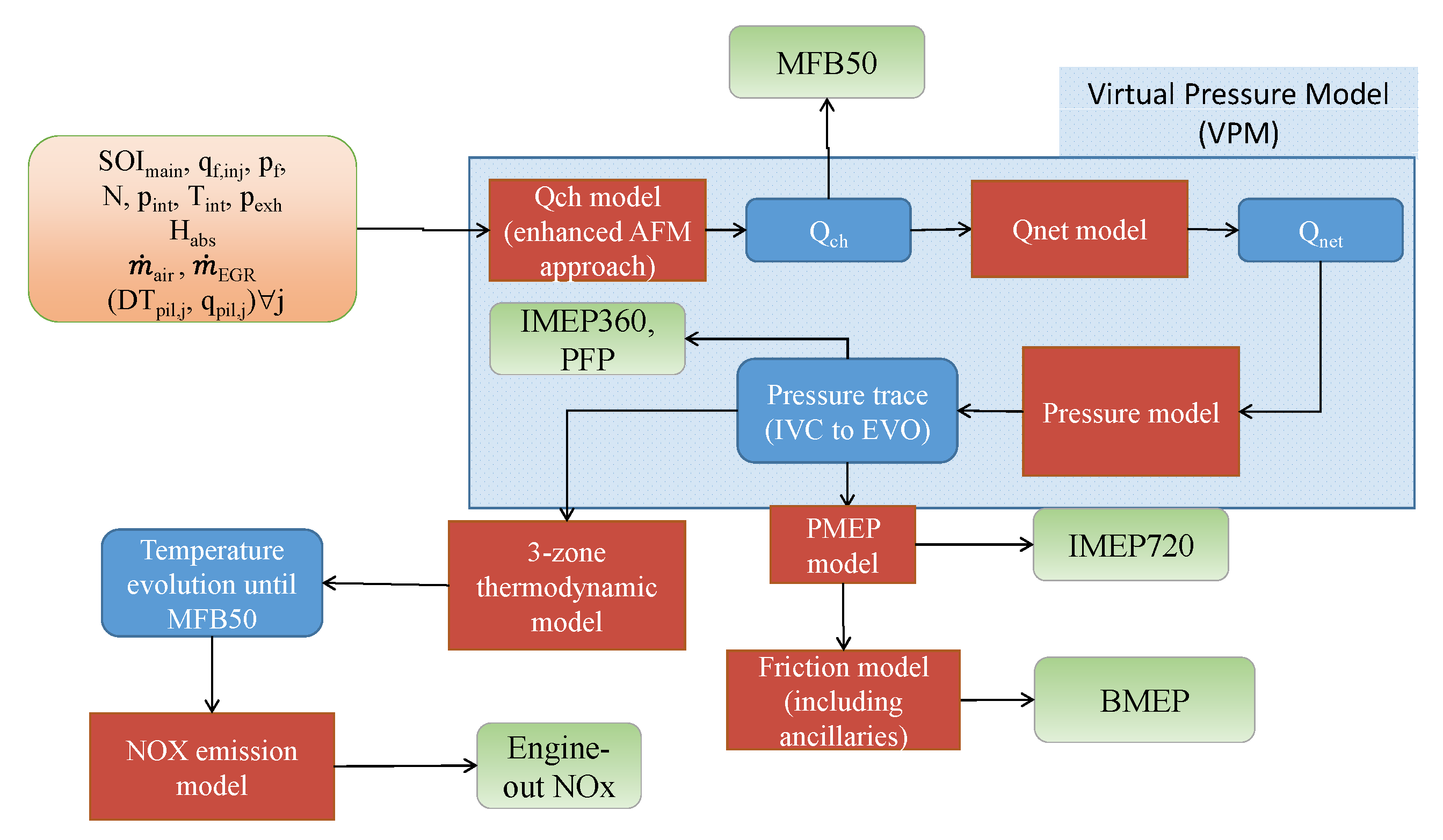
Figure 6 reports the scheme of the real-time combustion model. The detailed description of each sub-model is not here reported for the sake of brevity. However, a description of the chemical energy release model is reported in the next section, since the latter is used to estimate the MFB50 metric, which is one of the inputs that is required by the newly proposed NOx model.
Estimation of the Chemical Energy Release Qch and of MFB50
The chemical energy release model is reported in [29]. In particular, the chemical energy release rate of the pilot injections is estimated as follows:
where Kpil,j and τpil,j are the combustion rate coefficient and the ignition delay coefficient, respectively, and Qfuel,pil,j is the chemical energy of the mass of fuel which is injected.
Concerning the main injection, the following formulation was used:
The additional term in Equation (10) was included in order to increase the accuracy at medium-high load conditions [29].
The Qfuel term is estimated as follows:
where tSOI indicates the start of the injection time, tEOI the end of the injection time, HL is the lower heating value of the fuel and is the fuel mass rate.
The total chemical energy release is therefore:
The model was assessed for the steady-state conditions reported in Figure 3, by minimizing the error between the predicted and experimental trends of heat release and in-cylinder pressure. The following correlations were derived for the model parameters:
In Equations (14)–(18), ρSOI and ρSOC indicate the in-chamber densities evaluated at the start of injection or combustion, respectively, and are expressed in kg/m3. The injection pressure pf is expressed in bar, the engine speed N in rpm, the total injected fuel quantity qf,inj in mm3/cyc/cyl, the total injected fuel quantity of the pilot shots qpil,tot in mm3/cyc/cyl and finally the intake oxygen concentration O2 in %. pint indicates the intake manifold pressure.
MFB50 is finally estimated as the crank angle at which the 50% of the maximum chemical energy has been released.
3.5. Considerations Concerning Model Recalibration for Different Engines
Some considerations are reported hereafter concerning the model recalibration when applied to different engines. In general, the calibration of the NOx model requires the acquisition of:
- A full engine map with baseline operating parameters: this map is used in order to derive the nominal values of the NOx emissions, intake O2 concentration and MFB50 used in the model (see Equations (2)–(4)).
- Sweep tests of intake O2 concentration and injection parameters (e.g., SOImain, prail) at fixed key-points: these tests are required in order to identify the correlation of the NOx deviations (Equation (3)). The key-points should be located in the engine area in which a high accuracy in the NOx prediction is required.
In general, the number of sweep tests required for the model calibration is not high, since the model is physically robust. It will be shown in the paper that even in the case in which only 5% of the tests available for this study is used, the results do not deteriorate significantly. The same experimental tests can be used for the calibration of the heat release model, if a pressure sensor is not installed on the engine.
4. Evaluation of the Uncertainty of the Measured NOx and of the Predicted NOx
The procedure applied to evaluate the uncertainty was based on the recommended practices reported in [39]. A short summary is provided hereafter.
Given an output quantity y, which is dependent on N independent xi variables, the associated variance is obtained as follows:
Equation (19) is consistent if the mutual effects between independent variables are neglected. ci is defined as the “coefficient of sensitivity” of ‘y’ with respect to the i-th independent variable ‘xi’.
Once has been evaluated, it is possible, by assuming a level of confidence (e.g., 95%) and a correspondent coverage factor k (e.g., equal to 2), to evaluate the expanded combined uncertainty of y, i.e., :
The previous method has been used in this study in order to estimate the experimental uncertainty of the measured NOx emissions and the uncertainty of the proposed NOx model.
In particular, the expanded combined uncertainty Uc of the measured NOx concentration had already been carried out in [20], and is reported here for the sake of completeness. This uncertainty mainly depends on two contributions: the uncertainty of the NOx concentration of the span gas included in the calibration cylinders and the accuracy of the NOx measuring instrument (i.e., the CLD device). Two ranges (low-NOx/high-NOx) were used for the calibration of the CLD device that was used for the measurement of the NOx concentration in the exhaust gases: the low-NOx calibration range was realized using a calibration cylinder with a NOx concentration of 150 ppm in the span gas, while the high-NOx calibration range was realized using a calibration cylinder with a NOx concentration of 1000 ppm in the span gas. Table 4 reports the uncertainty of the NOx concentration in the span gas included in the calibration cylinders (Table 4a), the accuracy specifications of the CLD device (Table 4b) and the uncertainty of the measured NOx emissions considering four different levels (Table 4c).
With reference to the uncertainty of the NOx model, the procedure reported by Equations (19) and (20) was applied to the model expressed by Equations (2)–(4). In order to predict the model uncertainty, it is necessary to estimate a reasonable variance of the input quantities. The results of this analysis are reported in the Results and Discussion section.
5. Model Calibration
The NOx model given by Equations (2)–(4) has been calibrated using all the tests reported in Figure 3. The tuning was done by means of the by means of the least square method. The resulting expression of NOx deviation (i.e., Equation (2)) is the following one:
The positive coefficients of the δMFB50 terms are in line with the observations reported in Section 3.3, while the positive exponent of the ‘qf,inj’ term means that the NOx deviation range increases with engine load. The effect of engine speed is, instead, less significant than that of the injected fuel quantity, and opposite for positive or negative variations of MFB50.
6. Results and Discussion
In this section the proposed NOx model will be assessed and validated at both steady-state conditions (Section 6.1) and transient operation (Section 6.2). It should be recalled that the input variables of the model are MFB50, intake O2 concentration, engine speed and total injected fuel quantity.
Considering that MFB50 can be either derived from the in-cylinder pressure trace (if the engine is equipped with pressure transducers), or estimated by a predictive heat release model (i.e., Equations (9)–(18)), both cases have been considered for the model assessment. With reference to the case in which MFB50 is extracted from the in-cylinder pressure trace, the values of MFB50 used in the model are the result of the average over the last consecutive 100 cycles for the steady-state tests, while they derive from a cycle-by-cycle acquisition in the transient tests. The intake O2 concentration used in the model was taken from the measurements of the gas analyzer (an intake O2 sensor was not available), while engine speed and total injected quantity were taken from the test bench measurements.
With reference to the intake O2 concentration, the values used in the model were the result of an average over the last 60 s for the steady-state tests (an engine stabilization time of 30–60 s is carried out before the measurement of each steady-state point). For the transient tests, the instantaneous intake O2 concentration was used in the model, in which the acquisition frequency was equal to 20 Hz.
The results have also been compared with those of the semi-empirical model previously reported in [8].
Section 6.3 reports a sensitivity study focused on the impact of the number of points used for calibration on the model accuracy. This analysis will demonstrate that the proposed model is robust even when a very low number of points is used for calibration, thus it is physically consistent.
In Section 6.4, the results related to the model uncertainty are shown. Section 6.5 will be focused on the impact of the uncertainty in the intake O2 estimation on the accuracy of the predicted NOx levels. Finally, Section 6.6 is focused on the results concerning the required computational time on the ETAS ES910 rapid prototyping device.
6.1. Model Assessment at Steady-State Conditions
First, the model has been assessed for the steady-state tests reported in Figure 3. Figure 7 reports the predicted vs. experimental levels of NOx emissions (ppm). In particular, Figure 7a reports the results of the NOx model (Equations (2)–(4)) when MFB50 is estimated from the in-cylinder pressure sensor, Figure 7b reports the results of the NOx model when MFB50 is estimated by the predictive heat release model (Equations (9)–(18)), and finally Figure 7c reports the results of the previous NOx model reported in [8].
The prediction accuracy of each model has been quantified by the squared correlation coefficient (R2) and by the Root Mean Squared Error (RMSE), which are reported in each figure.
It can be seen in the figure that, for the proposed NOx model, the RMSE value is of the order of 34 ppm when MFB50 is estimated through the pressure sensor, and of the order of 44 ppm when MFB50 is estimated by the heat release model. In both cases, the accuracy is of the same order as that of the previously developed model [8], i.e., 38 ppm.
6.2. Model Validation over Transient Conditions
The model has then been validated in transient conditions. The results reported in this section are related to six sets of up/down speed/load ramps of different duration. Figure 8 reports the time histories of the engine speed and torque for the six analyzed sets of ramps. The variation range of engine speed was between 1600 rpm and 2500 rpm, while the variation range of engine torque was between 55 Nm and 215 Nm. The duration of the first three sets of ramps was 5 s, while the duration of the remaining three sets of ramps was 3 s. It can be seen in Figure 8 that the first test is constituted by a ramp-up and a ramp-down of both engine speed and torque, the second test is constituted by a ramp-up and a ramp-down of torque at fixed engine speed, while the third test is constituted by a ramp-up and a ramp-down of speed at fixed engine torque. The three sets of ramps have then been repeated by reducing the ramp duration to 3 s.
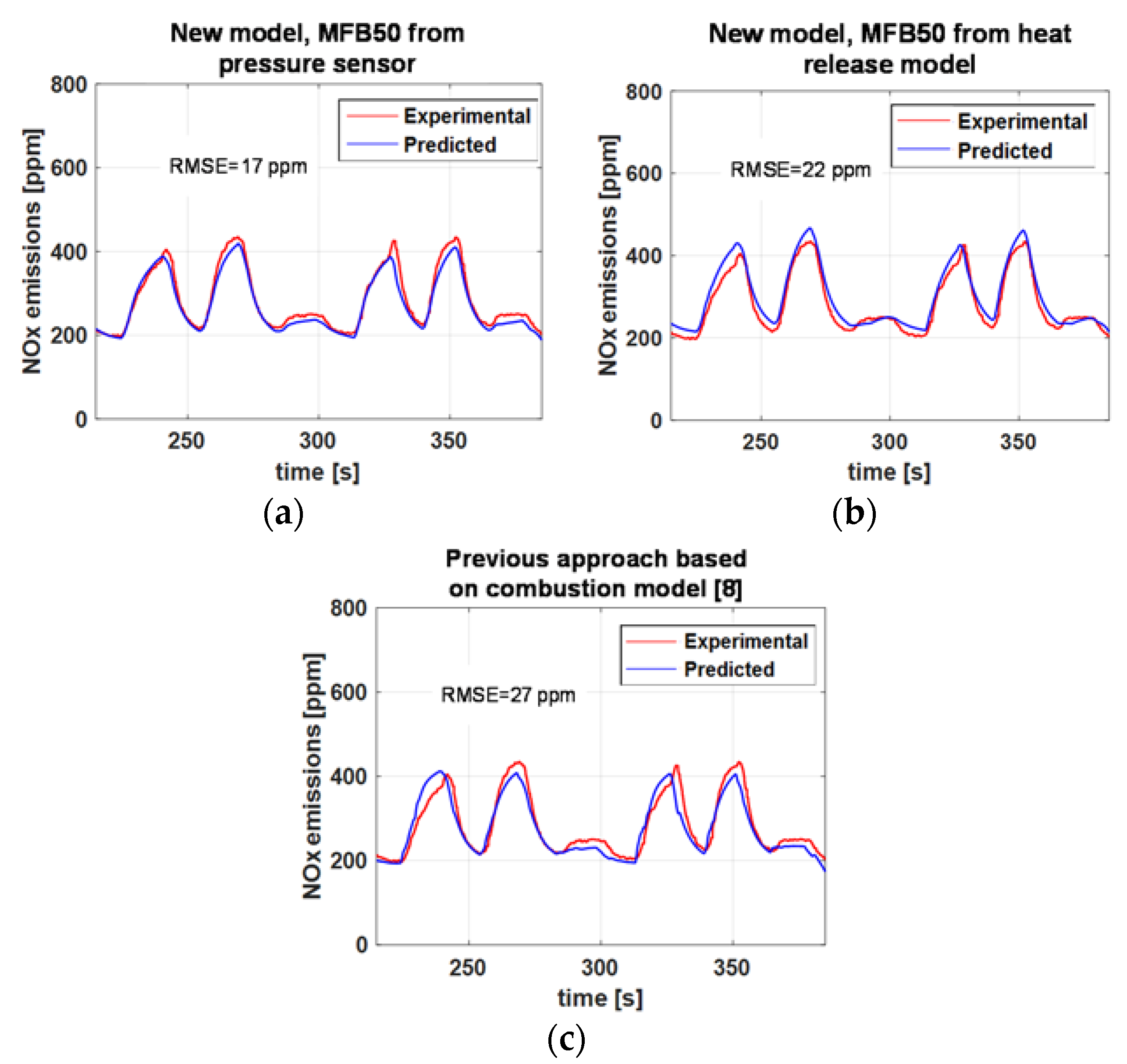
The main model results have been reported in Figure 9. In particular, the figures report the predicted and experimental values of the instantaneous engine-out NOx emissions over the considered ramps. In all the charts, the experimental values have been reported in red color, while the results of the model have been reported in blue color. The values of RMSE are also reported at the top of each graph.
More in detail, Figure 9a reports the predicted NOx trends using the NOx model, in which MFB50 was estimated through the in-cylinder pressure sensor, Figure 9b reports the predicted NOx trends using the NOx model, in which MFB50 is estimated by the predictive heat release model, and finally Figure 9c reports the predicted NOx levels using the previous NOx model reported in [8].
It should be noted that the predicted NOx trends that are reported in Figure 9 are the result of a filtering of the predicted raw trends, adopting a time constant τc = 5 s. This filtering is necessary for the comparison with the experimental trends, since the latter are obtained from the measurements of the gas analyzer, which suffers from a certain degree of smoothing and delaying (compared to the actual engine-out NOx levels over the transient), due to the mixing of the exhaust gases in the pipes that connect the engine to the gas analyzer. This effect had already been observed in [8]. In order to have an experimental measurement of the NOx emissions that is more representative of the actual dynamics which occurs in the engine exhaust manifold, a NOx sensor with high frequency response (not available for the considered tests) should be installed in the engine.
It can be seen in Figure 9a,b that the new NOx model is highly accurate over the considered transient tests, and its accuracy is of the same order of that of the previous approach [8] based on the predictive combustion model (Figure 9c). The accuracy of the proposed NOx model is good even when MFB50 is not extracted from the in-cylinder pressure sensor, but is estimated by the predictive heat release model (see Figure 9b).
6.3. Model Calibration with Limited Number of Experimental Tests
In this section, a sensitivity analysis of the model accuracy, with respect to the number of tests used for calibration, has been carried out. In particular, the original calibration dataset was reduced progressively (a random point selection was realized). The model was tuned for each reduced dataset, and applied to the whole dataset, and the accuracy was estimated through the RMSE parameter. The result of this analysis is reported in Table 5 for the steady-state tests, and in Table 6 for the transient tests.
It can be observed in the tables that the accuracy of the model is not significantly influenced by the percentage of points used for calibration. The slight reductions in the RMSE values that may occur when reducing the number of tests can be justified considering that the reduced datasets were generated randomly. The model outcomes are still acceptable when only 5% of available points are used for the model tuning, at both steady-state and transient conditions.
6.4. Analysis of the NOx Model Uncertainty
An analysis of the uncertainty of the proposed model has been carried out, according to the procedure reported in Section 4. Each of the model parameter (i.e., MFB50, O2, N, qf,inj), in general, is in fact characterized by a variance, which determines an uncertainty in the predicted NOx levels.
It was verified that MFB50 and O2 lead to the highest contribution in the uncertainty of the predicted NOx emissions, while the contribution of N and qf,inj is smaller (the maximum error of the encoder is of the order of 0.00075 N, while the error of the fuel meter is of the order of 0.1% of the measured value).
Two cases have been considered for this analysis:
- Case 1: MFB50 is estimated from the in-cylinder pressure sensor.
- Case 2: MFB50 is estimated by the predictive heat release model.
Table 7 reports the standard deviation σ of MFB50 and O2 that was adopted for the two cases.
The standard deviation of MFB50 that is associated to case 1 was derived using the information related to the accuracy of the pressure transducer, while the standard deviation of MFB50 that is associated to case 2 was obtained by means of a statistical analysis of the heat release model accuracy.
With reference to the intake O2 concentration, the standard deviation was obtained on the basis of the accuracy of the Paramagnetic Oxygen Detector (POD) device that is installed in the gas analyzer, and on the basis of the uncertainty in the gas concentration of the calibration cylinders.
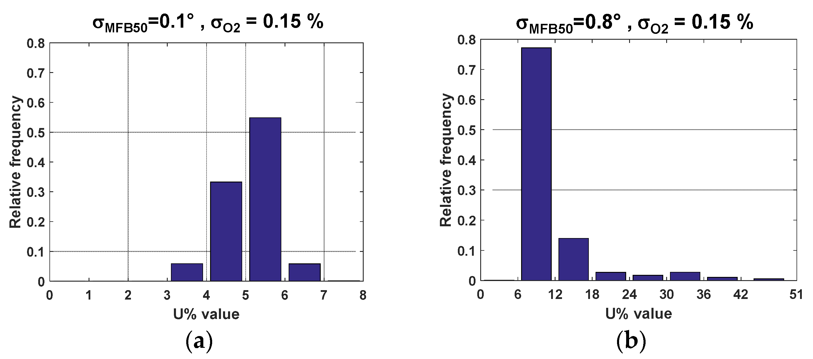
Figure 10 reports the results of this analysis. In particular, Figure 10a,c report, for the steady-state tests of Figure 3, the upper and lower values bands of the predicted NOx emissions taking into account the expanded uncertainty ‘Uc’ (i.e., NOx + Uc and NOx − Uc). Figure 10a refers to case 1 (MFB50 from pressure sensor), while Figure 10c refers to case 2 (i.e., MFB50 from heat release model). The values of the standard deviation of MFB50 and O2 are reported on the top of each chart. For the same two cases, Figure 10b,d report the statistical distributions of the relative expanded uncertainty of the predicted NOx emissions.
It can be seen from the charts that the use of an in-cylinder pressure sensor to estimate MFB50 (with a standard deviation σ = 0.1°) can lead to a relative uncertainty in the predicted NOx emissions that is between 2 and 8%, while the use of the heat release model to estimate MFB50 (with a standard deviation σ = 0.8°) leads to a relative uncertainty that is between 5% and 25%.
The uncertainty analysis has also been carried out for the transient tests reported in Figure 8. Figure 11 reports the statistical distributions of the relative expanded uncertainty of the predicted NOx emissions for case 1 (MFB50 from pressure sensor, Figure 11a) and case 2 (i.e., MFB50 from heat release model, Figure 11b).
It can be seen that, for the analyzed transient tests, the use of an in-cylinder pressure sensor to estimate MFB50 (with a standard deviation σ = 0.1°) can lead to a relative uncertainty in the predicted NOx emissions that is between 3% and 7%, while a broader distribution of uncertainty occurs if a heat release model is used to estimate MFB50 (with a standard deviation σ = 0.8°).
6.5. Impact of Intake O2 Error on the NOx Prediction Accuracy
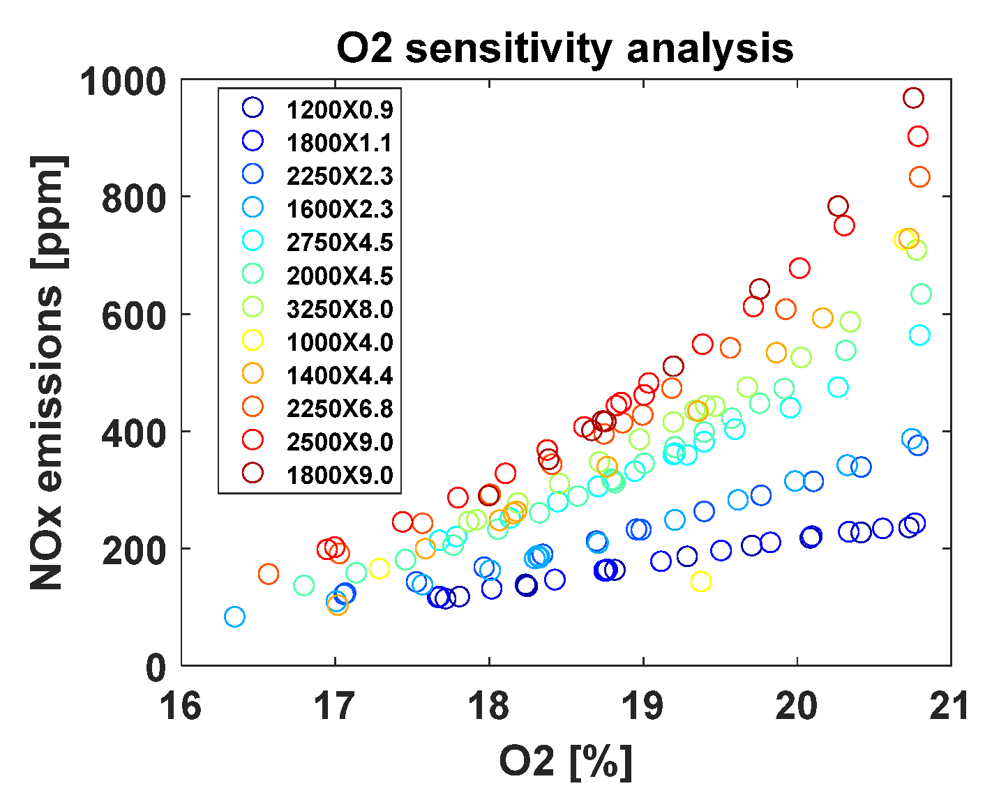
The intake oxygen concentration has a great impact on the NOx emissions. This can be observed in Figure 12, which reports, for the EGR sweep tests of Figure 3, the measured NOx emissions as a function of the measured intake O2 concentration.
It can be seen that the sensitivity increases with engine load: for the engine point N = 1800 rpm, BMEP = 9 bar, a variation of 1% of intake O2 leads to a variation of NOx emissions that is of the order of 200 ppm.
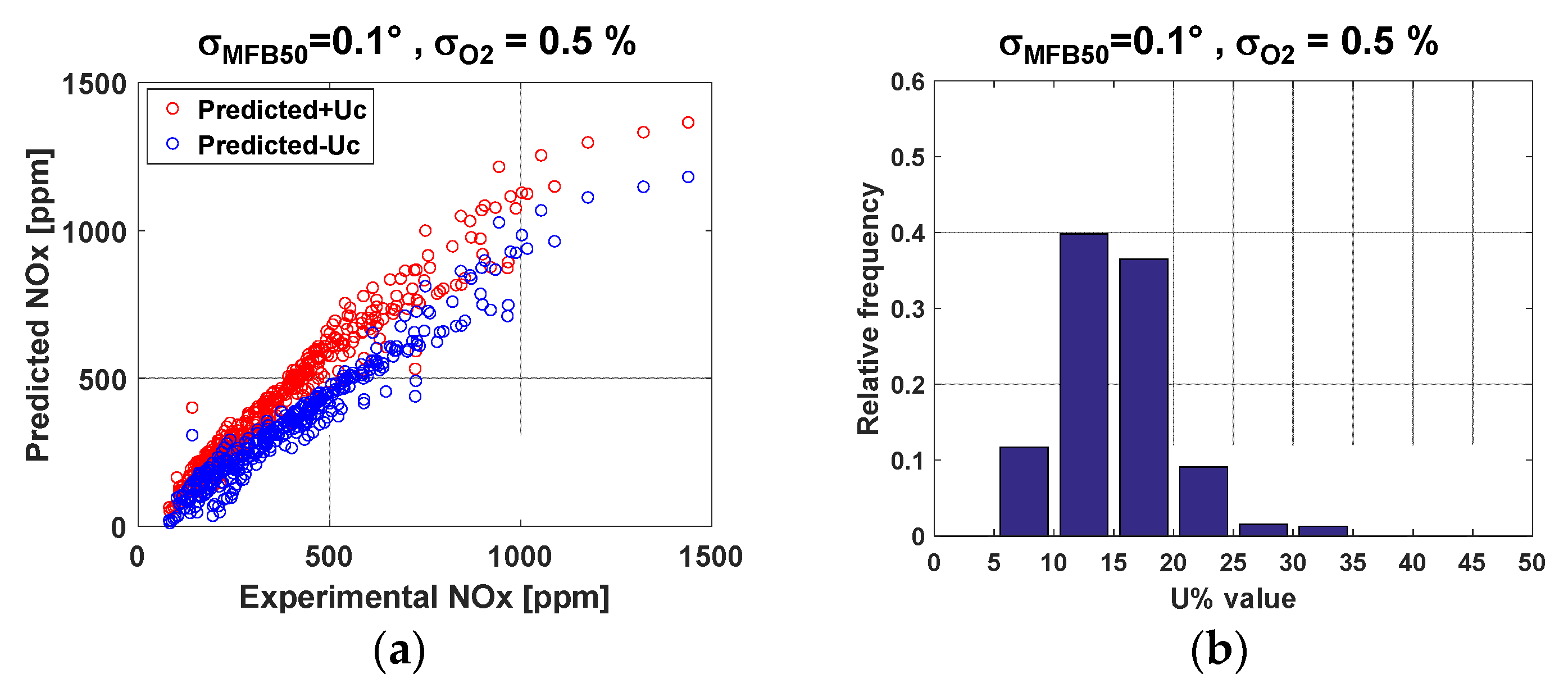
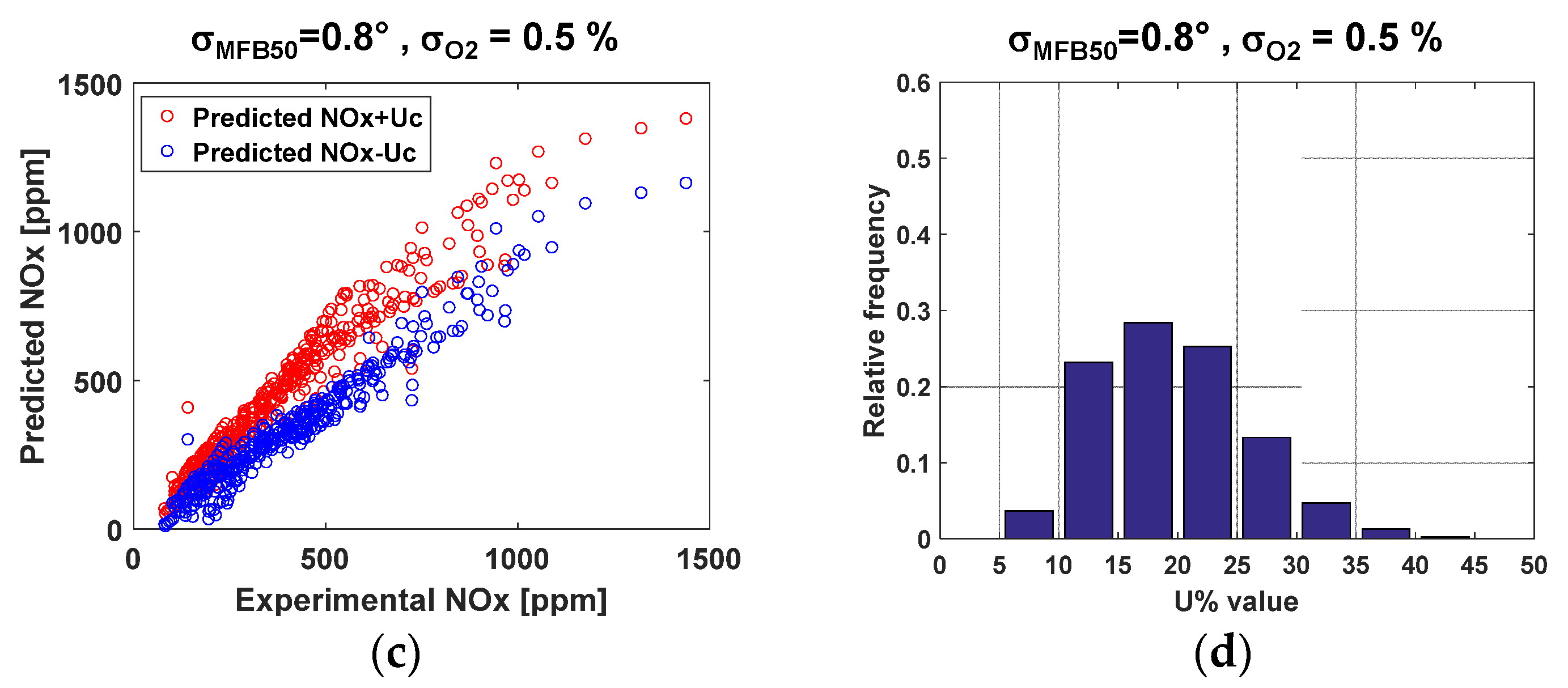
In order to evaluate the impact, on the uncertainty of the NOx model, of a case in which the variance in the intake O2 estimation is high, the analysis carried out in the previous section has been repeated by assuming a standard deviation σO2 = 0.5%. This standard deviation can be representative of the accuracy of intake O2 models typically adopted in ECUs. The results are reported in Figure 13. In particular, Figure 13a,c report, for the steady-state tests of Figure 3, the upper and lower values bands of the predicted NOx emissions taking into account the expanded uncertainty ‘Uc’ (i.e., NOx + Uc and NOx − Uc). Figure 13a refers to the case in which MFB50 is estimated from the pressure sensor, while Figure 13c refers to the case in which MFB50 is estimated by the heat release model. The values of the standard deviation σ are reported, for MFB50 and O2, on the top of each chart. For the same two cases, Figure 13b,d report the statistical distribution of the relative expanded uncertainty of the predicted NOx emissions.
It can be seen from the charts that if the standard deviation of the intake O2 is equal to 0.5%, the relative uncertainty of the predicted NOx emissions increases in a range between 5 and 25% if MFB50 is estimated by the pressure sensor (Figure 13b), while it increases in a range between 5 and 35% if MFB50 is estimated by the heat release model (Figure 13d).
This suggests that the adoption of an intake O2 sensor with high accuracy is recommended in order to have an accurate estimation of NOx emissions. An analysis of the current state of the art in the development of intake O2 sensors suggests that it is possible to achieve very high levels of accuracy which are stable over time. For example, the intake O2 sensor developed in [40] is characterized by a maximum relative error that is of the order of 2% (which corresponds to a standard absolute deviation σO2 = 0.2% for a measured value of intake O2 concentration equal to 20%, assuming that the maximum error has a coverage factor of 95%). This standard deviation is not far from that of the POD device that was used to validate the model in this paper (see the uncertainty analysis in the previous section).
6.6. Required Computational Time on ETAS ES910
The new NOx model was developed in Matlab/Simulink environment and was then implemented on a rapid prototyping (RP) device (i.e., ETAS ES910), through the ETAS Intecrio software, in view of a possible implementation for real-time NOx control. The aim of this investigation was to test the real-time capability of the NOx model, for the subsequent utilization in control-oriented tasks. The results of this investigation activity, in terms of computational time required by the model on the ETAS ES910 device per iteration, are shown in Table 8.
It can be seen that the new proposed NOx models require a much smaller computational time, when compared to the previous approach, in both cases in which MFB50 is estimated by a pressure sensor or from the heat release model. This can be explained by the fact that the 3-zone thermodynamic model included in the predictive combustion model is highly time-consuming (see also [8]).
7. Conclusions
A new semi-empirical model has been developed to predict nitrogen oxides (NOx) emissions in a 3.0 L diesel engine at both steady-state and transient conditions. The model has been designed in order to require a low computational effort, and to be robust with respect to the input variable variance. The proposed method relies on the estimation of the deviations of NOx emissions, with respect to the nominal engine values, as a function of the deviations of the intake oxygen concentration and of the combustion phasing ‘MFB50’. The model also takes into account the effects of engine speed, total injected quantity, and ambient temperature and humidity.
The method has been developed and assessed for a Fiat Powertrain Technologies (FPT) Euro VI 3.0 L diesel engine for commercial applications, within the frame of a research project in collaboration with FPT Industrial.
The model accuracy has first been evaluated at steady-state conditions, considering engine map tests, EGR sweep test and sweep tests of injection pressure and injection timing. The overall accuracy is quite high, since the RMSE values are of the order of 35 and 45 ppm when the combustion phasing is estimated through an in-cylinder pressure sensor or by a heat release model, respectively.
The model has then been tested in transient operation, over several ramps of speed and load, and demonstrated to be accurate, since the RMSE values are of the order of 20 ppm.
An uncertainty analysis was also carried out, in order to evaluate the impact of the input variable variance on the predicted NOx variance.
It was found that the variance of the NOx model can be quite good (2–8%), if the intake O2 concentration is measured with a sufficiently level of accuracy (e.g., with a standard deviation of 0.15%).
The model has also been tested on a rapid prototyping device, and it was shown that it requires a very short computational time, thus being suitable for implementation on the Engine Control Unit (ECU) for real-time NOx control tasks.
Author Contributions
Omar Marello conceived the combustion model, performed the simulations and took part in the acquisition of the experimental data; Roberto Finesso gave support for the experimental test planning and for the model development, and wrote the paper under the supervision of Ezio Spessa; Gilles Hardy supervised the research along with Ezio Spessa, provided technical support for the activity and revised the paper; Claudio Maino provided support for the paper revision and proofreading. Ezio Spessa supervised the research activity.
Conflicts of Interest
The authors declare no conflict of interest.
Abbreviations
| BMEP | Brake Mean Effective Pressure |
| c | Coefficient of sensitivity |
| CA | Crank angle |
| CFD | Computer fluid-dynamics |
| CLD | Chemiluminescence detector |
| DT | Dwell-time |
| ECU | Engine control unit |
| EGR | Exhaust gas recirculation |
| EOI | End of injection |
| EVO | Exhaust valve opening |
| FPT | Fiat powertrain technologies |
| Habs | Absolute humidity of the air |
| HCCI | Homogeneous charge compression ignition |
| HL | Lower heating value of the fuel |
| ICEAL-PT | Internal Combustion Engines Advanced Laboratory at the Politecnico di Torino |
| IMEP | Indicated mean effective pressure |
| IMEP360 | Gross indicated mean effective pressure |
| IMEP720 | Net indicated mean effective pressure |
| IVC | Intake valve closing |
| K | Combustion rate coefficient |
| m | Mass |
| MAF | Mass airflow sensor |
| mfuel | Total injected fuel mass per cycle/cylinder |
| Fuel injection rate | |
| MFB50 | Crank angle at which 50% of the fuel mass fraction has burned |
| N | Engine rotational speed |
| O2 | Intake charge oxygen concentration |
| p | Pressure |
| PCCI | Premixed charge compression ignition |
| pexh | Exhaust manifold pressure |
| pf | Injection pressure |
| PFP | Peak firing pressure |
| pint | Intake manifold pressure |
| PMEP | Pumping mean effective pressure |
| POD | Paramagnetic oxygen detector |
| q | Injected fuel volume quantity |
| Qch | Chemical heat release |
| qf,inj | Total injected fuel volume quantity per cycle/cylinder |
| Qfuel | Chemical energy associated with the injected fuel |
| Qnet | Net heat release |
| qpil | Injected fuel volume quantity of the pilot injection |
| qpil,tot | Total injected fuel volume quantity of the pilot injections |
| R2 | Squared correlation coefficient |
| RMSE | Root mean square error |
| SOC | Start of combustion |
| SOI | Electric start of injection |
| SOImain | Electric start of injection of the main pulse |
| t | Time |
| T | Temperature |
| Tamb | Ambient temperature |
| Tbmax,main | Maximum temperature of the burned gas zone during the combustion of the main pulse |
| Tb,MFB50 | Temperature of the burned gas zone at MFB50 |
| Tint | Intake manifold temperature |
| u2 | Variance |
| Uc | Expanded combined uncertainty |
| VGT | Variable Geometry Turbine |
| VPM | Virtual Pressure Model |
| Greek symbols | |
| Stoichiometric charge-to-fuel ratio | |
| ρ | Density |
| ρSOI | In-chamber ambient density evaluated at the SOI instant |
| ρSOC | In-chamber ambient density evaluated at the SOC instant |
| σ | Standard deviation |
| τ | Ignition delay coefficient |
| Subscripts | |
| air | Made of air |
| EGR | Made of EGR |
| main | Main pulse |
| pil | Pilot pulse |
References
- Vlachos, T.G.; Bonnel, P.; Perujo, A.; Weiss, M.; Villafuerte, P.; Riccobono, F. In-use emissions testing with portable emissions measurement systems (PEMS) in the current and future european vehicle emissions legislation: Overview underlying principles and expected benefits. SAE Int. J. Commer. Veh. 2014, 7, 199–215. [Google Scholar] [CrossRef]
- Johnson, T. Vehicular emissions in review. SAE Int. J. Engines 2014, 7, 1207–1227. [Google Scholar] [CrossRef]
- Catania, A.E.; d’Ambrosio, S.; Finesso, R.; Spessa, E.; Cipolla, G.; Vassallo, A. Combustion system optimization of a low compression-ratio PCCI diesel engine for light-duty application. SAE Int. J. Engines 2009, 2, 1314–1326. [Google Scholar] [CrossRef]
- Baratta, M.; Finesso, R.; Misul, D.; Spessa, E. Comparison between Internal and External EGR Performance on a Heavy Duty Diesel Engine by Means of a Refined 1D Fluid-Dynamic Engine Model. SAE Int. J. Engines 2015, 8, 1977–1992. [Google Scholar] [CrossRef]
- Riegel, J.; Neumann, H.; Wiedenmann, H. Exhaust gas sensors for automotive emission control. Solid State Ion. 2002, 152–153, 783–800. [Google Scholar] [CrossRef]
- Mrosek, M.; Sequenz, H.; Isermann, R. Identification of emission measurement dynamics for diesel engines. IFAC Proc. Vol. 2011, 18, 11839–11844. [Google Scholar] [CrossRef]
- Manchur, T.; Checkel, M. Time Resolution Effects on Accuracy of Real-Time NOx Emissions Measurements; SAE Technical Paper 2005-01-0674; SAE International: Warrendale, PA, USA, 2005. [Google Scholar] [CrossRef]
- Finesso, R.; Hardy, G.; Marello, O.; Spessa, E.; Yang, Y. Model-Based Control of BMEP and NOx Emissions in a Euro VI 3.0 L Diesel Engine. SAE Int. J. Engines 2017, 10, 2288–2304. [Google Scholar] [CrossRef]
- Finesso, R.; Spessa, E.; Yang, Y.; Conte, G.; Merlino, G. Neural-Network Based Approach for Real-Time Control of BMEP and MFB50 in a Euro 6 Diesel Engine; SAE Technical Paper 2017-24-0068; SAE International: Warrendale, PA, USA, 2017. [Google Scholar] [CrossRef]
- Egnell, R. Combustion diagnostics by means of multizone heat release analysis and No calculation. SAE Trans. J. Engines 1998, 107, 22. [Google Scholar] [CrossRef]
- Andersson, M.; Johansson, B.; Hultqvist, A.; Noehre, C. A Predictive Real Time NOx Model for Conventional and Partially Premixed Diesel Combustion; SAE Technical Paper 2006-01-3329; SAE International: Warrendale, PA, USA, 2006. [Google Scholar] [CrossRef]
- Finesso, R.; Spessa, E. A Real Time Zero-Dimensional Diagnostic Model for the Calculation of In-Cylinder Temperatures, HRR and Nitrogen Oxides in Diesel Engines. Energy. Convers. Manag. 2014, 79, 498–510. [Google Scholar] [CrossRef]
- Finesso, R.; Spessa, E. Real-Time Predictive Modeling of Combustion and NOx Formation in Diesel Engines under Transient Conditions; SAE Technical Paper 2012-01-0899; SAE International: Warrendale, PA, USA, 2012. [Google Scholar] [CrossRef]
- Seykens, X.; Baert, R.; Somers, L.; Willems, F. Experimental validation of extended no and soot model for advanced hd diesel engine combustion. SAE Int. J. Engines 2009, 2, 606–619. [Google Scholar] [CrossRef]
- Rao, V.; Honnery, D. A comparison of two NOx prediction schemes for use in diesel engine thermodynamic modeling. Fuel 2013, 107, 662–670. [Google Scholar] [CrossRef]
- Asprion, J.; Chinellato, O.; Guzzella, L. A fast and accurate physics-based model for the NOx emissions of Diesel engines. Appl. Energy 2013, 103, 221–233. [Google Scholar] [CrossRef]
- Asprion, J.; Chinellato, O.; Guzzella, L. Optimisation-oriented modelling of the NOx emissions of a Diesel engine. Energy Convers. Manag. 2013, 75, 61–73. [Google Scholar] [CrossRef]
- Kim, G.; Moon, S.; Lee, S.; Min, K. Numerical Analysis of the Combustion and Emission Characteristics of Diesel Engines with Multiple Injection Strategies Using a Modified 2-D Flamelet Model. Energies 2017, 10, 1292. [Google Scholar] [CrossRef]
- Lucchini, T.; D’Errico, G.; Cerri, T.; Onorati, A.; Hardy, G. Experimental Validation of Combustion Models for Diesel Engines Based on Tabulated Kinetics in a Wide Range of Operating Conditions; SAE Technical Paper 2017-24-0029; SAE International: Warrendale, PA, USA, 2017. [Google Scholar] [CrossRef]
- D’Ambrosio, S.; Finesso, R.; Fu, L.; Mittica, A.; Spessa, E. A control-oriented real-time semi-empirical model for the prediction of NOx emissions in diesel engines. Appl. Energy 2014, 130, 265–279. [Google Scholar] [CrossRef]
- Krishnan, A.; Sekar, V.C.; Balaji, J.; Boopathi, S.M. Prediction of NOx reduction with exhaust gas recirculation using the flame temperature correlation technique. In Proceedings of the National Conference on Advances in Mechanical Engineering, Kota, India, 18–19 March 2006; pp. 378–385. [Google Scholar]
- Guardiola, C.; López, J.J.; Martin, J.; García-Sarmiento, D. Semiempirical in-cylinder pressure based model for NOx prediction oriented to control applications. Appl. Therm. Eng. 2011, 31, 2375–3286. [Google Scholar] [CrossRef]
- Arregle, J.; López, J.J.; Guardiola, C.; Monin, C. Sensitivity Study of a NOx Estimation Model for On-Board Applications; SAE Technical Paper 2008-01-0640; SAE International: Warrendale, PA, USA, 2006. [Google Scholar] [CrossRef]
- Lee, S.; Lee, Y.; Kim, G.; Min, K. Development of a Real-Time Virtual Nitric Oxide Sensor for Light-Duty Diesel Engines. Energies 2017, 10, 284. [Google Scholar] [CrossRef]
- Guardiola, C.; Martín, J.; Pla, B.; Bares, P. Cycle by cycle NOx model for diesel engine control. Appl. Therm. Eng. 2017, 110, 1011–1020. [Google Scholar] [CrossRef]
- Brace, C. Prediction of Diesel Engine Exhaust Emissions using Artificial Neural Networks. In Proceedings of the IMechE Seminar S591, Lucas Electrical and Electronic Systems-Neural Networks in Systems Design, Solihull, UK, 10 June 1988. [Google Scholar]
- Roy, S.; Banerjee, R.; Bose, P.K. Performance and exhaust emissions prediction of a CRDI assisted single cylinder diesel engine coupled with EGR using artificial neural network. Appl. Energy 2014, 119, 330–340. [Google Scholar] [CrossRef]
- Catania, A.E.; Finesso, R.; Spessa, E. Predictive zero-dimensional combustion model for DI diesel engine feed-forward control. Energy Convers. Manag. 2011, 52, 3159–3175. [Google Scholar] [CrossRef]
- Alfieri, V.; Conte, G.; Finesso, R.; Spessa, E.; Yang, Y. HRR and MFB50 Estimation in a Euro 6 Diesel Engine by means of Control-Oriented Predictive Models. SAE Int. J. Engines 2015, 8, 1055–1068. [Google Scholar] [CrossRef]
- Finesso, R.; Marello, O.; Misul, D.; Spessa, E.; Violante, M.; Yang, Y.; Hardy, G.; Maier, C. Development and Assessment of Pressure-Based and Model-Based Techniques for the MFB50 Control of a Euro VI 3.0L Diesel Engine. SAE Int. J. Engines 2017, 10, 1538–1555. [Google Scholar] [CrossRef]
- Heywood, J.B. Internal Combustion Engine Fundamentals; McGraw-Hill Intern: Columbus, OH, USA, 1988. [Google Scholar]
- Finesso, R.; Spessa, E. Estimation of the Engine-out NO2/NOx Ratio in a EURO VI Diesel Engine; SAE Technical Paper 2013-01-0317; SAE International: Warrendale, PA, USA, 2013. [Google Scholar] [CrossRef]
- Fenimore, C.P. Formation of nitric oxide in premixed hydrocarbon flames. Symp. Combust. 1971, 13, 373–380. [Google Scholar] [CrossRef]
- Zeldovich, Y.B.; Sadovnikov, P.Y.; Kamenetskii, D.A.F. Oxidation of Nitrogen in Combustion; Shelef, M., Translator; Academy of Sciences of USSR, Institute of Chemical Physics: Moscow-Leningrad, Russia, 1947. [Google Scholar]
- Lavoie, G.A.; Heywood, J.B.; Keck, J.C. Experimental and theoretical study of nitric oxide formation in internal combustion engines. Combust. Sci. Technol. 1970, 1, 313–326. [Google Scholar] [CrossRef]
- Miller, R.; Davis, G.; Lavoie, G.; Newman, C.; Gardner, T. A Super-Extended Zel’dovich Mechanism for NOx Modeling and Engine Calibration; SAE Technical Paper 980781; SAE International: Warrendale, PA, USA, 1998. [Google Scholar] [CrossRef]
- Hegarty, K.; Dickinson, P.; Cieslar, D.; Collings, N. Fast O2 Measurement Using Modified UEGO Sensors in the Intake and Exhaust of a Diesel Engine; SAE Technical Paper 2013-01-1051; SAE International: Warrendale, PA, USA, 1998. [Google Scholar] [CrossRef]
- Test Procedure for the Measurement of Gaseous Exhaust Emissions from Small Utility Engines; SAE J1088_201303 Recommended Practice; SAE International: Warrendale, PA, USA, 2013.
- ISO/IEC GUIDE 98–3:2008(E). Uncertainty of measurement. Guide to the expression of Uncertainty in Measurement; International Organization for Standardization: Geneva, Switzerland, 2008. [Google Scholar]
- 2015 DOE Annual Merit Review REGIS. Available online: https://energy.gov/sites/prod/files/2015/06/f23/ace091_schnabel_2015_o.pdf (accessed on 15 October 2017).
Figure 1.
FPT F1C 3.0 L Euro VI diesel engine installed on the highly dynamic test bench at the Politecnico di Torino. The EATS ES910 rapid prototyping device can be observed on the right side.
Figure 1.
FPT F1C 3.0 L Euro VI diesel engine installed on the highly dynamic test bench at the Politecnico di Torino. The EATS ES910 rapid prototyping device can be observed on the right side.

Figure 2.
Scheme of the test bench (a) and engine (b) including the location of the main sensors.
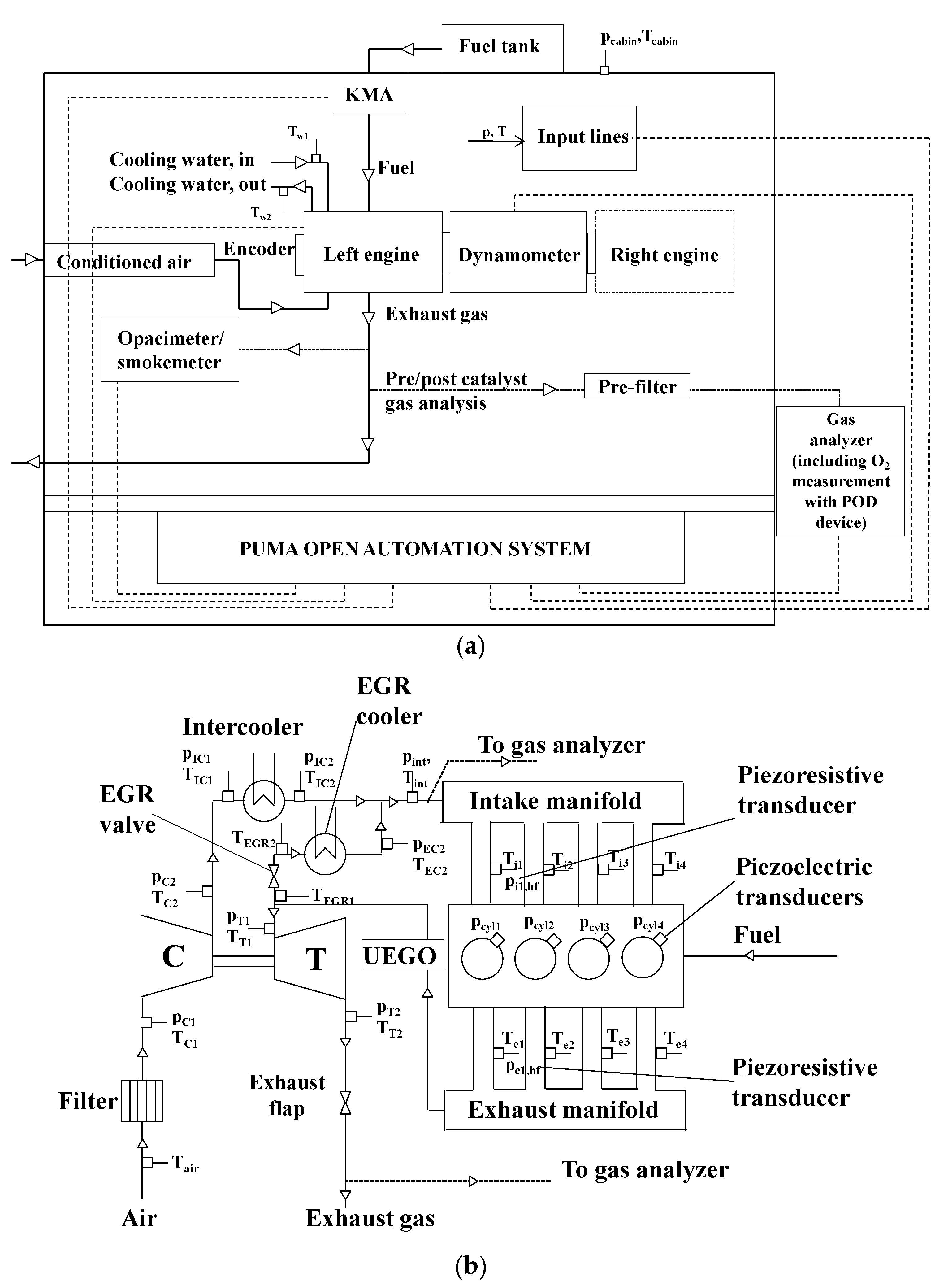
Figure 3.
Summary of the experimental tests.
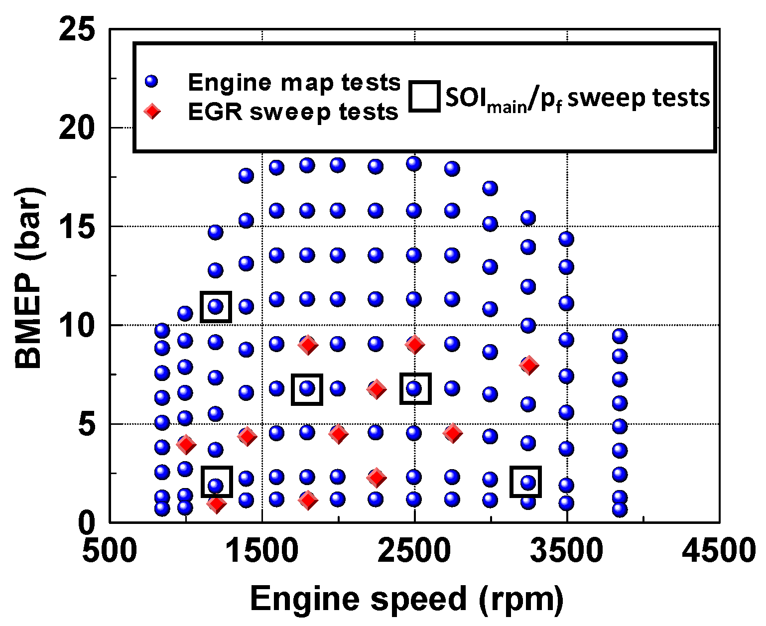
Figure 4.
Contour plots of measured NOx emissions as a function of injection pressure and SOImain, for the points indicated by the black squares.
Figure 4.
Contour plots of measured NOx emissions as a function of injection pressure and SOImain, for the points indicated by the black squares.
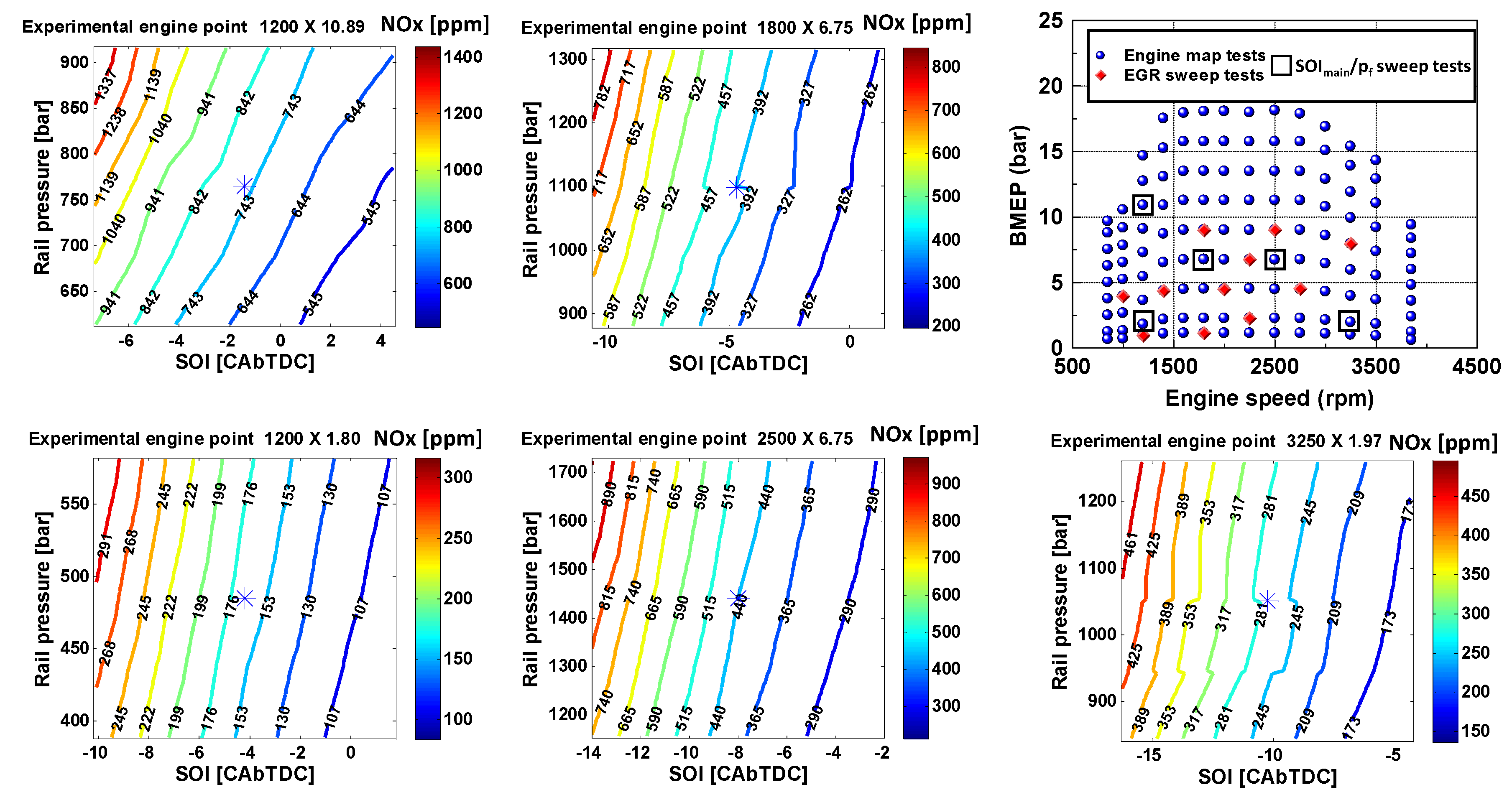
Figure 5.
Contour plots of measured NOx emissions as a function of injection pressure and MFB50, for the points indicated by the black squares.
Figure 5.
Contour plots of measured NOx emissions as a function of injection pressure and MFB50, for the points indicated by the black squares.
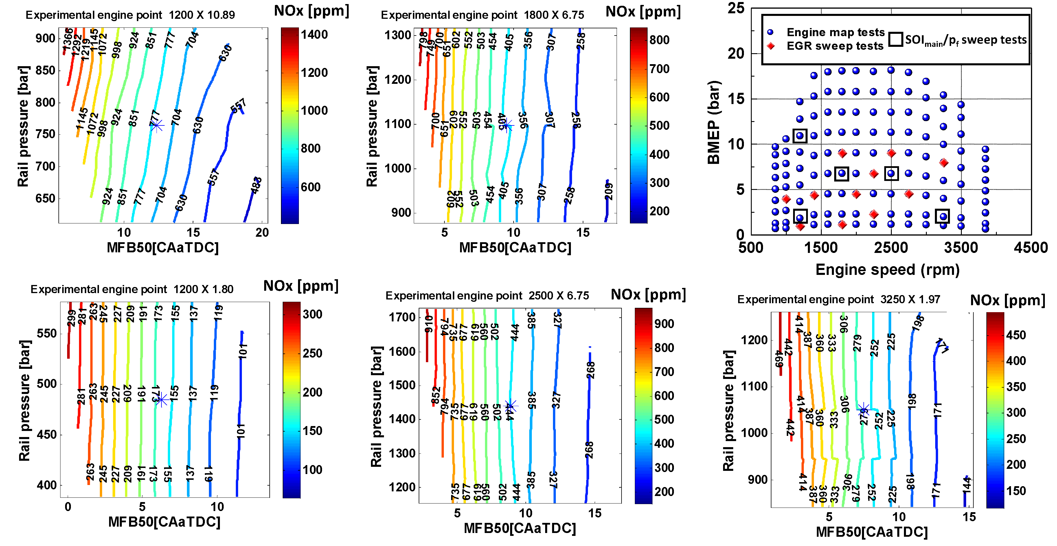
Figure 6.
Scheme of the predictive combustion model reported in [8].
Figure 6.
Scheme of the predictive combustion model reported in [8].

Figure 7.
Predicted vs. experimental values of engine-out NOx emissions for the steady-state tests reported in Figure 3; (a) new model, MFB50 from pressure sensor; (b) new model, MFB50 from heat release model; (c) NOx model presented in [8].

Figure 8.
Engine speed and torque as a function of time for the analyzed transient test.
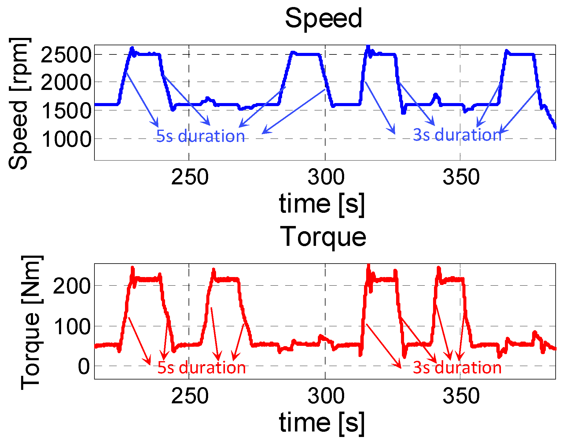
Figure 9.
Predicted and experimental trends of engine-out NOx emissions for the analyzed transient test. The predicted NOx trace has been filtered using a time constant of 5 s, as reported in [8]. (a) new model, MFB50 from pressure sensor; (b) new model, MFB50 from heat release model; (c) previous model presented in [8].

Figure 10.
Results of the uncertainty analysis of the NOx model for the steady-state tests of Figure 3, adopting a standard deviation σO2 = 0.15% (O2 from gas analyzer). (a,c) upper and lower values bands of the predicted NOx emissions taking into account the expanded uncertainty ((a) MFB50 from pressure sensor, (c) MFB50 from heat release model); (b,d) statistical distribution of the relative expanded uncertainty of the predicted NOx emissions ((b) MFB50 from pressure sensor, (d) MFB50 from heat release model).
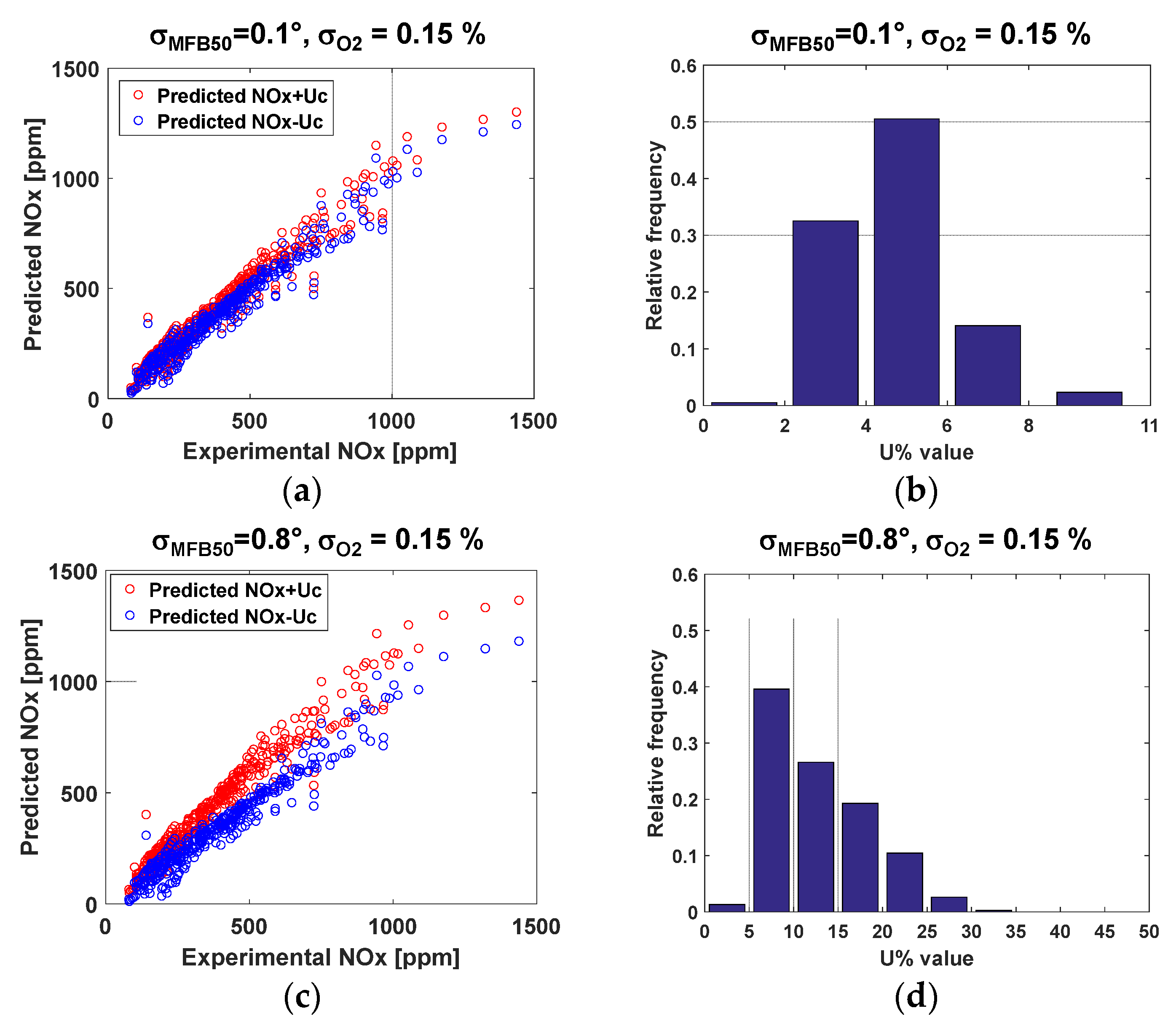
Figure 11.
Results of the uncertainty analysis of the NOx model for the transient test of Figure 8, adopting a standard deviation σO2 = 0.15% (O2 from gas analyzer). The statistical distribution of the relative expanded uncertainty of the predicted NOx emissions is reported ((a) MFB50 from pressure sensor, (b) MFB50 from heat release model).

Figure 12.
Measured NOx emissions as a function of the measured intake O2 concentration for the EGR sweep tests reported in Figure 3.
Figure 12.
Measured NOx emissions as a function of the measured intake O2 concentration for the EGR sweep tests reported in Figure 3.

Figure 13.
Results of the uncertainty analysis of the NOx model for the steady-state tests of Figure 3, assuming a standard deviation σO2 = 0.5% (e.g., O2 from model). (a,c): upper and lower values bands of the predicted NOx emissions taking into account the expanded uncertainty ((a) MFB50 from pressure sensor, (c) MFB50 from heat release model); (b,d): statistical distribution of the relative expanded uncertainty of the predicted NOx emissions ((b) MFB50 from pressure sensor, (d) MFB50 from heat release model).

Table 1.
Main technical specifications of the engine.
| Engine Specifications | |
|---|---|
| Engine type | FPT F1C Euro VI diesel engine |
| Number of cylinders | 4 |
| Displacement | 2998 cm3 |
| Bore × stroke | 95.8 mm × 104 mm |
| Rod length | 160 mm |
| Compression ratio | 17.5 |
| Valves per cylinder | 4 |
| Turbocharger | VGT type |
| Fuel injection system | High pressure Common Rail |
Table 2.
Main specifications of the ETAS ES910 device.
| ETAS ES910 Device | |
|---|---|
| Main processor | Freescale PowerQUICCTM III MPC8548 with 800 MHz clock Double precision floating point unit |
| Memory | 512 MByte DDR2-RAM (400 MHz clock) |
| 64 MByte Flash | |
| 128 kByte NVRAM | |
Table 3.
Main properties of the diesel EN590 fuel.
| Property | Units | Diesel EN 590 |
|---|---|---|
| Cetane number | - | 53.1 |
| Flash Point | °C | 70 |
| Density at 15 °C | kg/m3 | 844 |
| Viscosity at 40 °C | mm2/s | 2.860 |
| Lower heating value | MJ/kg | 43.4 |
Table 4.
(a) Uncertainty of NOx calibration cylinders. (b) Main sources of error of the CLD device. (c) Expanded uncertainty of the measured NOx for different measured values.
Table 4.
(a) Uncertainty of NOx calibration cylinders. (b) Main sources of error of the CLD device. (c) Expanded uncertainty of the measured NOx for different measured values.
| (a) | ||
| Measuring Range | NOx Concentration in the Span-Gas of the Calibration Cylinder | Relative Expanded Uncertainty Uc |
| low-NOx | 150 ppm | 2% |
| high-NOx | 1000 ppm | 2% |
| (b) | ||
| Error type | Error | |
| Linearity | ≤2% of measured value (10–100% of full scale range) | |
| ≤1% of full scale range whichever is smaller | ||
| Drift 24 h | ≤1% of full scale range | |
| Reproducibility | ≤0.5% of full scale range | |
| (c) | ||
| Measured NOx | Uc | Relative Uc |
| 50 ppm | 1.6 ppm | 3.1% |
| 100 ppm | 2.5 ppm | 2.5% |
| 500 ppm | 16 ppm | 3.3% |
| 1300 ppm | 33 ppm | 2.5% |
Table 5.
Values of RMSE related to the prediction of NOx emissions, as a function of the percentage of data used for the model calibration, when applying the model to the steady-state tests reported in Figure 3.
Table 5.
Values of RMSE related to the prediction of NOx emissions, as a function of the percentage of data used for the model calibration, when applying the model to the steady-state tests reported in Figure 3.
| % of Tests Used for Calibration | NOx RMSE (MFB50 from Pressure Sensor) | NOx RMSE (MFB50 from Heat Release Model) |
|---|---|---|
| 100 | 34 ppm | 44 ppm |
| 50 | 34 ppm | 44 ppm |
| 25 | 36 ppm | 46 ppm |
| 20 | 37 ppm | 45 ppm |
| 15 | 38 ppm | 45 ppm |
| 10 | 40 ppm | 46 ppm |
| 5 | 46 ppm | 53 ppm |
Table 6.
Values of RMSE related to the prediction of NOx emissions, as a function of the percentage of data used for the model calibration, when applying the model to the transient test reported in Figure 8.
Table 6.
Values of RMSE related to the prediction of NOx emissions, as a function of the percentage of data used for the model calibration, when applying the model to the transient test reported in Figure 8.
| % of Tests Used for Calibration | NOx RMSE (MFB50 from Pressure Sensor) | NOx RMSE (MFB50 from Heat Release Model) |
|---|---|---|
| 100 | 17 ppm | 22 ppm |
| 50 | 16 ppm | 23 ppm |
| 25 | 14 ppm | 27 ppm |
| 20 | 14 ppm | 27 ppm |
| 15 | 15 ppm | 25 ppm |
| 10 | 13 ppm | 28 ppm |
| 5 | 18 ppm | 18 ppm |
Table 7.
Standard deviation of MFB50 and O2 for the evaluation of the uncertainty of the NOx model.
| Input Parameter | Case 1 (MFB50 from Pressure Sensor) | Case 2 (MFB50 from Heat Release Model) |
|---|---|---|
| MFB50 | σ = 0.1° | σ = 0.8° |
| O2 | σ = 0.15% | σ = 0.15% |
Table 8.
Average computational time required by the NOx models, when implemented on the ETAS ES910 RP device.
Table 8.
Average computational time required by the NOx models, when implemented on the ETAS ES910 RP device.
| New NOx (MFB50 from Pressure Sensor) | New NOx Model (MFB50 from Heat Release Model) | NOx Model Presented in [8] |
|---|---|---|
| <50 μs | ~200–300 μs | ~1500 μs |
© 2017 by the authors. Licensee MDPI, Basel, Switzerland. This article is an open access article distributed under the terms and conditions of the Creative Commons Attribution (CC BY) license (http://creativecommons.org/licenses/by/4.0/).
Share and Cite
MDPI and ACS Style
Finesso, R.; Hardy, G.; Maino, C.; Marello, O.; Spessa, E. A New Control-Oriented Semi-Empirical Approach to Predict Engine-Out NOx Emissions in a Euro VI 3.0 L Diesel Engine. Energies 2017, 10, 1978. https://doi.org/10.3390/en10121978
AMA Style
Finesso R, Hardy G, Maino C, Marello O, Spessa E. A New Control-Oriented Semi-Empirical Approach to Predict Engine-Out NOx Emissions in a Euro VI 3.0 L Diesel Engine. Energies. 2017; 10(12):1978. https://doi.org/10.3390/en10121978
Chicago/Turabian StyleFinesso, Roberto, Gilles Hardy, Claudio Maino, Omar Marello, and Ezio Spessa. 2017. "A New Control-Oriented Semi-Empirical Approach to Predict Engine-Out NOx Emissions in a Euro VI 3.0 L Diesel Engine" Energies 10, no. 12: 1978. https://doi.org/10.3390/en10121978
Note that from the first issue of 2016, this journal uses article numbers instead of page numbers. See further details here.