Using a Local Framework Combining Principal Component Regression and Monte Carlo Simulation for Uncertainty and Sensitivity Analysis of a Domestic Energy Model in Sub-City Areas

Abstract

Domestic energy modelling is complex, in terms of user input and the approach used to define the model; therefore, there is an increase in the sources of uncertainties. Previous efforts to perform sensitivity and uncertainty analyses have focused on national energy models, while in this research, the objective is to extend traditional sensitivity analysis and use a local framework combining principal component regression and Monte Carlo Simulation. Therefore, in our method the total amount of the energy output’s variance is decomposed, in relative terms, according to the contribution of the different predictor parameters. Our framework provides compelling evidence that local area characteristics are important in energy modelling and those national and regional indexes and values may not properly reflect the local conditions, resulting in programmes and interventions that will be sub-optimal. Furthermore, our uncertainty methodology uses a three dimensional integrative taxonomy and a concept map. The concept map identified concrete terminal causes of uncertainty within the taxonomic framework of sources, issues, sub-issues and a further abstraction of those quantities in terms of accuracy and precision. Understanding uncertainties in this way provides a possible framework for modellers, policy makers and data collectors to improve practice in key areas and to reduce uncertainty.

1. Introduction

Despite the importance of the domestic energy modelling in sub-city areas, the energy sector lacks a rigorous analytical framework to account for the uncertainties. The most common practice is to assign a single uncertainty value to the modelled output. We develop a taxonomy (Taxonomy comes from the Greek taxis meaning arrangement or order, and monos meaning law/science (or knowledge)) that shows how uncertainties are propagated through the modelling process (data—model—refinement—validation) and in the resulting estimates of annual energy consumption. Furthermore, our concept map lays out all these factors in a common diagram, so that energy modelling in sub-city areas can be better understood and synchronized in other cities.

In the last ten years, we found interesting research dealing with uncertainty and sensitivity of energy models, and advanced statistics, examples are: Eisenhower et al. extended traditional sensitivity analysis in order to decompose the pathway as uncertainty flows through the dynamics and identified which internal or intermediate processes transmit the most uncertainty to the final output [1]; Grömping assigned shares of “relative importance to each of a set of regressors when applying linear regression” [2] and Nguyen et al. employed several sensitivity analysis methods commonly used in building simulation to assess the significance of various input parameters in specific mathematical models and computer building energy models [3]. Summerfield et al. argue that uncertainty appears in domestic energy modelling as follows: (i) input data, both in terms of the accuracy of the individual input entry and the range of values associated with a particular building component; (ii) in assumptions about the energy calculation engine, or inaccuracies in the values implicitly assumed in the calculation for the weather characteristics surrounding the building, among other assumptions; (iii) in differences between the measures ‘as modelled’ and the specification ‘as constructed’; (iv) in differences in the occupancy patterns; and; (v) in issues with post-occupancy surveying and monitoring of the building [4]. Additionally, Rubin argue that if the individual dwelling energy results are to be aggregated within the sub-city areas, then all of the dwelling profiles for the whole area have to be filled; if not, issues of missing data become important [5].

Our paper provides a tri-dimensional taxonomy of uncertainty using a concept map. Our concept map requires the identification of the sources, issues and sub-issues of the uncertainties in the modelling process. In addition to the taxonomic structure, due to variations in energy phenomena that need to be numerically calculated, this paper also considers data distributions reflecting the uncertainty available to allow the use of numerical simulation methods for uncertainty quantification and propagation. For this uncertainty analysis, therefore, it is possible to use methods such as those based on Monte Carlo analysis due to variations in phenomena that can be numerically calculated.

For the sensitivity analysis of the input variables, our paper uses, in Section 3 and Section 4, a framework which combines principal component regression and Monte Carlo Simulation Method. The principle of Monte Carlo Simulation is the propagation of the input (predictors) probability distributions through the model. This provides a general probabilistic basis for uncertainty evaluation in the energy estimation outcome. Monte Carlo Simulation is used as a method to study the uncertainty propagation through the model. This study uses a dimensional approach opposite to a categorical approach to synthesis [6]. The advantages of using our framework are to explore many combinations of energy predictors and analyze all possible outcomes for significantly more accurate results and to identify the factors with the most impact, i.e., identify the factors in the energy predictors with the greatest impact on energy consumption. Our framework, see Section 4.2, uses the gas consumption of bungalows in Castle, a particular district in Newcastle upon Tyne, a city in the north east of England. Our proposed framework is quite general. Thus, it can be presented as a ‘local energy model’ as an applicative example.

This paper follows our previous work [7] using the Newcastle upon Tyne Carbon RouteMap Modelling Framework (NCRF). NCRF inherited the Newcastle Carbon Route Map (NCRM) [8], which is an early incarnation of a building level data set for Newcastle. The initial phase of this research involved substantial data management, cleaning, restructuring and additions to this initial data set. The resultant data set incorporated, in a single database table, a large number of building-related data sets. NCRF utilises this data set and adds to the energy modelling aspect through linking with the English House Survey (EHS) as input to the Cambridge Housing Model (CHM). This provides the means to produce building-level energy consumption estimates which in turn can be analysed both spatially and aspatially (e.g., by building type).

2. The Uncertainty Characterization

This section introduces the uncertainty characterization, but first introduces the two broad types of uncertainty: parametric and structural uncertainty; then suggests a relationship between the number of predictors (and their accuracy) in the accuracy of the model output. These two concepts, types and accuracy, are important to understand as this approach is used to frame the uncertainty and sensitivity in further sections.

Hickman et al. argues that the term uncertainty has been used to describe two different high level concepts where uncertainty can be found, the parameters and the structure [9]. Parametric (aleatory) uncertainty is the random variability in some parameter or measurable quantity, and structural (epistemic) uncertainty is an imprecision in the knowledge about a model, or its estimates. The distinction between these two concepts indicates that in the case of structural uncertainty, this can be decreased if there is an effort in data gathering that improves the quality of decision making and therefore reduces the uncertainty, but this cannot affect the fundamental random variability of the individual parameters.

When modelling sub-city areas, many parameters (or predictors) of the household real characteristics, the physical dwelling, the energy system and the close environment have to be set. However, when there is low information (e.g., household behaviour), usually designers choose to set several predictors with standard parameters in the structure of the model. If these standard parameters do not fit with the local area characteristics, a discrepancy between the modelled and measured energy consumption is observed. Therefore, we have to consider the structural uncertainties in the model. In the example, there are two main user behaviour parameters that influence the energy balance of the building: the indoor air temperature and the air exchange rate. The air exchange rate is caused by the infiltration, leakages in the building envelope, and the opening of windows and doors, these two effects are not completely separated and usually difficult to disaggregate. Consequently, they are presented in models as the total amount of air exchanged between the inner and the external space. To gain a better insight into this uncertainty, at least two options are available: either modify the existing model structure or use a systematic variation of the input predictors. The aim ‘modifying the structure’ is to change the model equations for every parameter, which is not desirable; therefore, extending, or changing, the original existing model [10] requires an impressive amount of modelling effort for all the parameters that use a standard definition and actual data to fill in. For the second option, which is the one used in this paper, it is possible to use the ‘standard model’ and apply a systematic variation of the input parameters to a Monte Carlo simulation method. In the Monte Carlo Simulation method (see Section 4), the probability distributions of the uncertain parameters are derived from measured data. Then, random numbers, for every uncertain parameter, are drawn from these distributions and combined to ‘one set of parameter inputs’ and applied trough the model description to gain an increased understanding of the relationships between predictors and the energy output variables.

Over this increased data gathering effort, Chapman argues that the rate of error in data input increases linearly with increasing data requirements, i.e., the more data that are measured and entered, the chances are that they could generate more errors, and the accuracy of a model increases with the logarithm of the number of data items required, i.e., the benefit of additional data is less than their linear increment [11]. Accuracy of the model means the degree to which the model could predict the estimates of energy given perfect data input, i.e., redundant (or dependent) input data do not improve the linear accuracy of the model. In short, adding more data makes things worse.

Figure 1 provides a Venn diagram [12] to illustrate the organization within the uncertainty characterization space and lists some of the specific methods for each subset: uncertainty quantification and uncertainty propagation.

The main terms defined in Figure 1 and in use in this paper are: uncertainty characterization, uncertainty quantification, and uncertainty propagation. The meaning of each of these terms is as follows [12]: ‘Uncertainty characterization is any proposition (declaration) that measures, quantitatively or qualitatively, the degree of uncertainty associated with a parameter and prediction; Uncertainty quantification is a subset of the uncertainty characterization in which only quantitative measures (in this research probabilistic density functions) are defined for uncertain parameters and predictions; Uncertainty propagation means making inferences about the uncertainty characterization in the output predicted parameters (model results) based on the uncertainty characterization of the input parameters’.

The techniques for propagating uncertainties can generally be classified [13] as intrusive or non-intrusive. Intrusive methods require reformulating the mathematical physical model. Non-intrusive methods use ensembles of simulations, where simulation ensemble members are created by assigning a probability density to the uncertain NCRF inputs according to various schemes that match each input in the sample. The impact of the input uncertainties and the model are analysed for the NCRF energy outcome, i.e., the annual energy consumption of that individual property type. This paper uses a non-intrusive uncertainty propagation method, because even though it is possible to modify the framework equations, this will require an impressive amount of modelling effort for all the predictors that use standard definitions. In the rest of this section, uncertainty propagation will assume non-intrusive uncertainty propagation.

The stochastic nature of the NCRF samples makes it necessary to estimate the probability density function of the output of the model from the statistical distribution for each of the model parameters, and a technique for propagating uncertainties (the Monte Carlo simulation method). The Monte Carlo simulation method is a problem-solving technique used to approximate the probability of certain outcomes (consequences) by running multiple trial runs, called simulations, using random variables.

The next section presents the key uncertainties in the energy model using a particular taxonomy originally used in the medical field [14]. The taxonomy clarifies the uncertainty by classifying systems in terms of concepts of knowledge, a graph (for plotting) these concepts and a hierarchy. The hierarchy links terms of a membership relation and a connectivity arrow joins each of the selected concepts to a source. This paper uses a hierarchical taxonomy to understand the uncertainty characterization in the NCRF domestic energy processes.

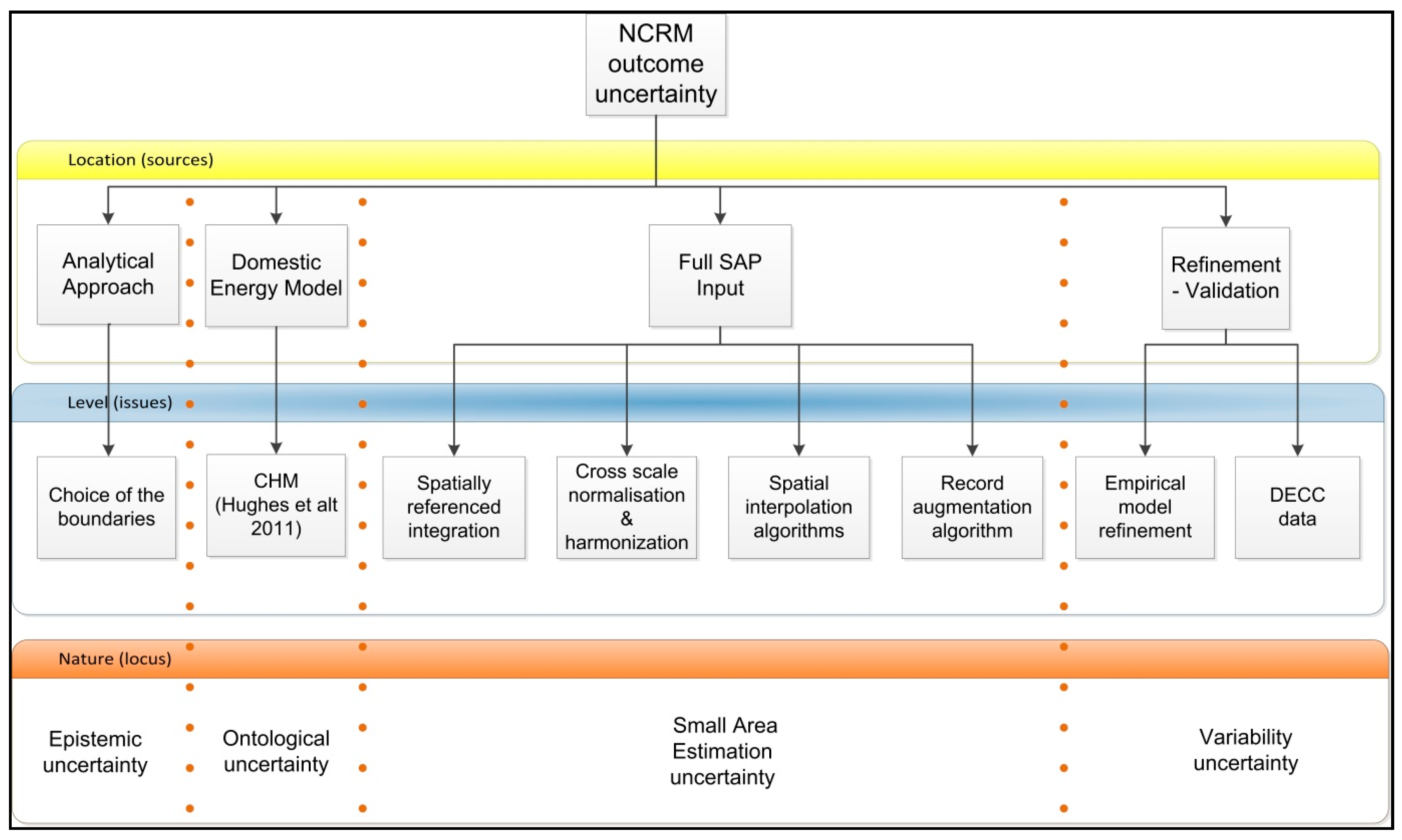
2.1. A Taxonomy of Key Uncertainties Using High-Level Frameworks

This section proposes a three dimensional integrative taxonomy of uncertainty representing a conceptual framework that helps to organize our knowledge by drawing our attention to relevant sources, issues and the nature of uncertainty in the NCRF estimates. This section shows how uncertainties are propagated through the modelling process (data—model—refinement—validation) and in the resulting estimates of annual energy consumption.

Figure 2 shows a three dimension integrative taxonomy of the uncertainty adapted from [14] by identifying the nature (location), the cause (level) and the extent (nature) of the uncertainty. The first dimension is the location (source) dimension of uncertainty that relates to where the uncertainty manifests within the complex energy model; the second dimension is the level (issues) dimension of uncertainty that relates to where the substantive issues (and from there the sub issues if meaningful) of uncertainty manifest along the whole spectrum between deterministic knowledge and total ignorance; and the third dimension is the nature (locus) dimension of uncertainty which relates to whether the uncertainty is due to the lack of knowledge or is due to the inherent variability of the variable being described.

The model outcome uncertainty in Figure 2 is the accumulated uncertainty caused by the uncertainties in all of the locations (context, model, inputs to the energy model, and refinement) that are propagated through and are reflected in the resulting estimates of annual energy consumption (aggregated in geographic boundaries or repeated for the same property type, floor area and year of construction). This uncertainty outcome could be considered a prediction error, since it is different from the United Kingdom’s Department of Energy and Climate Change (DECC) median value. As DECC values for energy consumption are known, a validation exercise was carried out to compare the median DECC value (as the true value) and NCRF predicted values in order to establish the prediction error.

Figure 2 accounts for the aggregate of uncertainties in all sources. However, it should be noted that NCRF could be used as an energy policy analysis model and estimate energy at other boundaries where there is no aggregation (beyond DECC known values), i.e., to estimate annual energy consumption outcomes for aggregated (or repeated) situations where DECC values are not publicly available. For those cases, the taxonomy shown in Figure 2 is still valid.

In Figure 2, the uncertainty issues are related to the methodology of the energy estimations. The first dimension ‘Location’ of uncertainty refers to: analytical approach, domestic energy model, full SAP (The UK Government’s Standard Assessment Procedure for the Energy Rating of Dwellings (SAP) was developed by Building Research Establishment (BRE) based on the BRE Domestic Energy Model (BREDEM) and was published by BRE and the Department of the Environment in 1992) input and refinement/validation. This section explains the three dimensions associated with the ‘analytical approach’, leading to Section 2.2 based on the uncertainty in the other sources identified, namely, the ‘domestic energy model’, ‘full SAP input’ and ‘refinement/validation’.

The analytical approach refers to the conditions and circumstances that underlie the choice of the boundaries of the system, the framing of the concepts and the terminology of the research question to be addressed within those boundaries. In this paper, the term analytical approach refers to the following issues: (i) the energy model and (ii) the size of the data space occupied by a model [15], which is related to its complexity. The NCRF energy estimates correspond to an engineering method which calculates the energy consumption of end-uses for dwellings based on the heat transfer and thermodynamic properties. Model complexity arises from the fact that NCRF has multiple inputs at different scales. It has two data sets at a resolution of the individual dwelling, one data set of rough approximations of household occupancy and three average regional scale landscape and climatic data sets.

The third dimension of the uncertainty is the nature of uncertainty. An important feature of uncertainty is the distinction between: (i) epistemic uncertainty (the uncertainty due to the imperfection of our knowledge), which may be reduced by doing more research and using added empirical efforts; and (ii) variability uncertainty, which is due to the inherent variability of the data. Between these two extremes, there is ‘ontological uncertainty’, which can be seen as having a semi-structured uncertainty, and ‘small area estimation uncertainty’, which can be seen as having a semi-variability uncertainty, as shown in columns of Figure 2.

The arrows in Figure 2 associate the NCRF outcome uncertainty with the first dimension sources, and in turn associate each source with its issues. The figure also presents the outer left source analytical approach having a structural (epistemic) uncertainty in the locus third dimension and from there an increasing parametric uncertainty, at the far right, with the refinement, i.e., the validation source.

CHM uses standard parameters that do not fit with the local area characteristics, then a discrepancy between the modelled and measured energy consumption can be observed. This means that this paper has to consider the structural uncertainties in the taxonomy of Figure 2. Also, the ‘CHM model’ is an idealized model of the domestic stock, and there is the possibility of an undetected error in the design that introduces ‘ontological uncertainty’. As an example, CHM does not consider some energy saving/generation technologies like the small-scale hydro-electric generator which is being considered in SAP 2009. The introduction of technologies that might be unfamiliar to the CHM model may carry a higher degree of ontological uncertainty.

The input data to CHM correspond to a full SAP data set. The cross-study analysis, spatial interpolation methods for asserting parameters, and the record augmentation strategy show how this paper performs indirect estimates from secondary sources (EHS, UK Census) in a city sample. The output estimation is the underlying expected value for any area given the independent variables included in the NCRF estimates and not the real value for the ‘small area’ in question. For this reason, as this is not a direct measure of the constructed SAP record for each dwelling in the city, but rather an estimation for each building, it can be considered as numeric uncertainty, i.e., towards the righthand side in Figure 2.

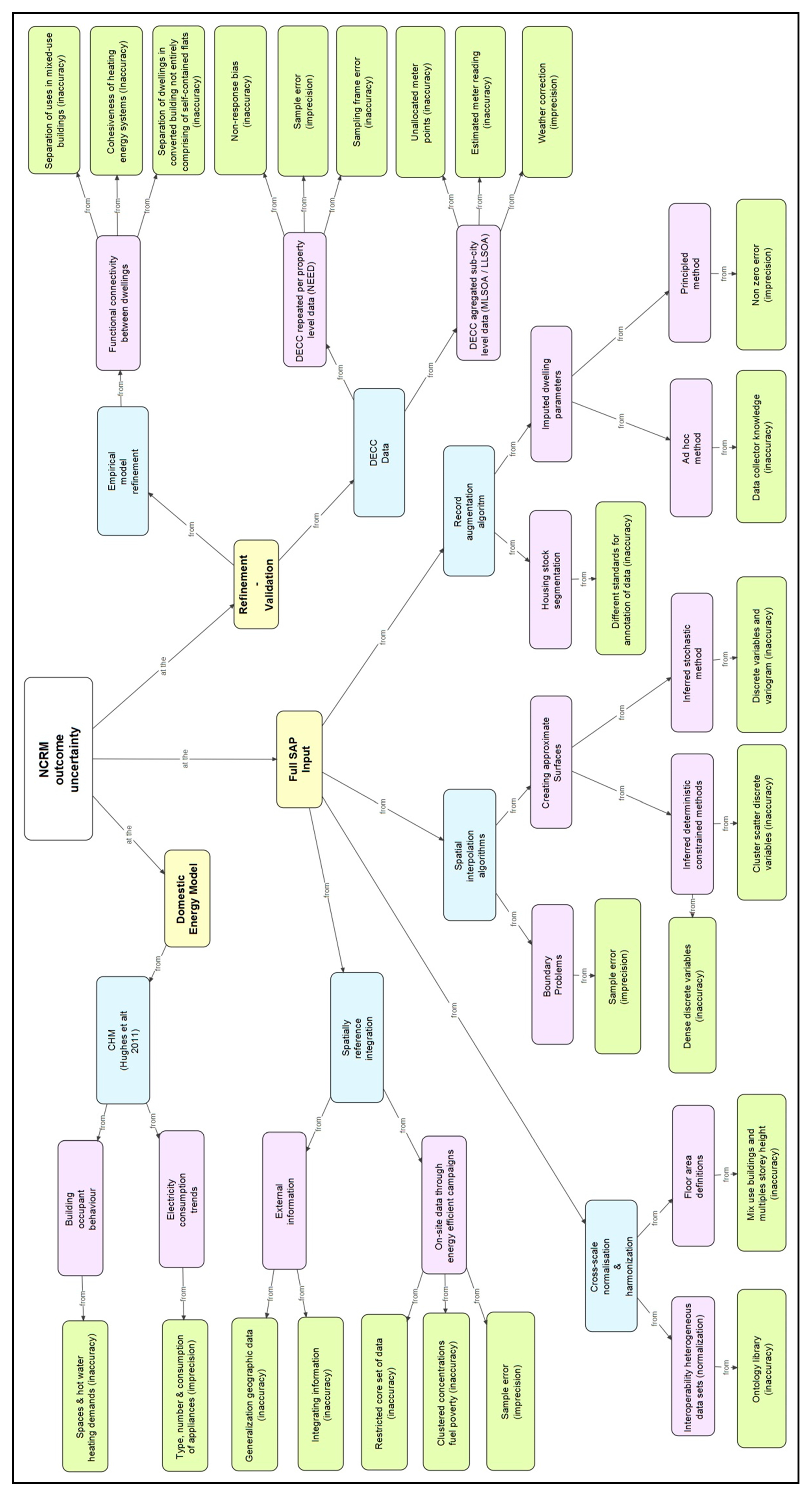
2.2. The NCRF Outcome Parametric Uncertainty Using a Concept Map

This section explains the second dimension (issues) for the sources of parametric uncertainty using a concept map. The idea is to show the key issues that connect and relate to the main sources of uncertainty and rank them with the most general, with inclusive issues coming first, and then links to smaller, more specific concepts until it reaches the quantification of the uncertainty in terms of an inaccuracy or imprecision. The concept map (CM) is proposed as a human friendly knowledge-representation of uncertainties, and is a tool especially defined for application in the learning process. It is easy to create, and is flexible and intuitive for people to understand [16,17,18].

The formalization in a CM of the quantified parametric uncertainties in the NCRF outcome is presented in Figure 3. Figure 3 is an extension of a previous work published on the uncertainties of the CHM [19] (see [19] for the uncertainties in this source model). This paper uses the CHM uncertainty model as a starting point for an emerging spatial, area-based urban, domestic energy model of uncertainties. Figure 3 shows the CM section derived from [19] plus the additional CM sections describing uncertainty sources from NCRF: ‘Full SAP input’ and ‘refinement/validation’.

In Figure 3, the green colour corresponds to the sources of uncertainties, and orange represents the issues (activities and disagreements) causing the uncertainties in the corresponding sources. Purple represents the sub-issues (a logically visible subdivision of an issue) and finally the terminal slots in green represent a further abstraction of those quantities that cause uncertainty in terms of accuracy and precision. The accuracy is the degree of closeness of measurements (of a quantity) to that quantity's actual true value and the precision (also called the reproducibility or repeatability) is the degree to which repeated measurements under unchanged conditions show the same results.

From Section 2.1 and Section 2.2, the uncertainty taxonomy can be summarized according to few dominant factors: (i) the underlying assumptions about processes exogenous to the model (e.g., climate variables). This will reflect in regional average parameters to be entered into the model; (ii) the underlying assumptions about endogenous processes in the model (e.g., spatial interpolation). Because none of the district zones in Newcastle upon Tyne are homogeneous, the resulting algorithm produces different surface structures in complex areas; (iii) the assumption in judgements, such as the ontology of the CHM model, e.g., in the building occupant behaviour, cannot only be a function of the usable floor area as in the SAP; (iv) the simplifying assumptions in the structure, e.g., the sum of meter points or domestic energy consumption at the Lower Layer Super Output Area (LLSOA) level does not always equal the sum of meter points of domestic energy consumption at the associated Middle Layer Super Output Area (MLSOA) level due to unallocated meters; and, finally (v) different weather correction methodologies in Department of Energy and Climate Change (DECC)/National Energy Efficiency Data-Framework (NEED) and CHM lead to some discrepancies (inaccuracy), which probably vary somewhat from year to year, because the exact methodology for weather correction for NEED/DECC is not fully disclosed.

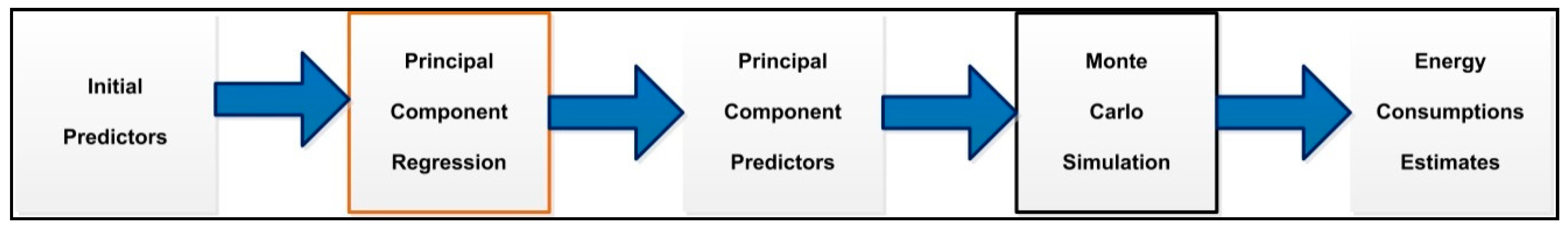
3. Framework Combining Principal Component Regression and Monte Carlo Simulation

Cullen and Frey argue that probabilistic sensitivity analysis explores two potentially important outcomes: first, the shift in the central tendency of a model results due to the shape in the distribution for the model inputs [20]. Comparing the results of the analysis, it is possible to identify subsets of input that have a profound influence on the central tendency of the output. Second, when principal components have been used to identity inputs which are significant contributions to output variance, the output variance may change, and, therefore, the relative importance of different sources of variability needs to be assessed.

Examples of Monte Carlo simulations for probabilistic modelling are being used in the field of nutrition; an example is the Office of Food Additive Safety (OFAS) (OFAS is in the Office of Food and Drug Administration (FDA) in the United States) that uses the Monte Carlo simulation to calculate percentile intakes for substances [21]. These simulations generate results for models in which several inputs can be defined by a distribution of values. Rather than using a single value for an input, the simulation selects a value at random from the distribution of possible values for that input, and uses that value to calculate an outcome for the model; also, Matthys et al. uses a probabilistic modelling of dietary exposure to micronutrients [22].

The probabilistic sensitivity analysis is used in this paper to assess the relative importance of model input predictors in the variance and central tendency of the energy consumption in a sample. The output from the Monte Carlo simulation is a range of possible outcomes from which a probability distribution function is prepared. The rest of the paper deals with a ‘what if scenario’ sensitivity framework. In this framework, the importance is in how the uncertainty of the NCRF gas consumption of bungalows can be explained in terms of the different sources of uncertainties.

For the energy consumption estimates (y), two types of different although related questions can be asked: (i) what is the uncertainty in the y(x) given the uncertainty in the n predictors x? And (ii) how important are the individual elements of x with respect to the uncertainty in y(x)? The goal of uncertainty analysis is to answer the first question, and the goal of sensitivity analysis is to answer the second question. However, the analysis of both is very closely connected. Helton et al. argue that the basic components that underlie the implementation of a sampling-based uncertainty and sensitivity analysis are: [23] (i) the definition of distributions D₁, D₂, …, D_n that characterize the elements x₁, x₂, …, x_n of x; (ii) the sample x₁, x₂, …, x_n, obtained from the x in consistency with the distributions D₁, D₂, …, D_n; (iii) propagation of the sample through the analysis to produce a mapping [x_i, y(x_i)], for i between 1 and n; (iv) the presentation of uncertainty analysis results (i.e., approximations to the distributions of the elements of y constructed from the corresponding elements of y(x_i); and (v) the determination of sensitivity analysis results (i.e., exploration of the mapping [x_i, y(x_i)], for i between 1 and n). In this paper only probabilistic characterizations of uncertainty are considered. Alternative uncertainty representations [24] are outside the scope of this paper.

For the definition of the distributions D₁, D₂, …, D_n, this is typically done through an expert review process [25] and is shown in Section 4. For the sample, the control of correlations is an important aspect of sample generation; specifically, correlated variables should have correlations close to their specified values, and uncorrelated variables should have correlations close to zero: in this paper a random sample was chosen from the NCRF and the correlations found in the principal component analysis. The propagation of the sample through the analysis to produce the mapping [x_i, y(x_i)], for i between 1 and n, is often the most computationally demanding part of a sampling based uncertainty and sensitivity analysis. This paper uses regression analysis [23] to provide an algebraic representation of the relationships between y and one or more of the x_i. Regression analysis is usually assumed to involve the construction of linear models of the form ŷ = b₀ + b_ix_i. For purposes of sensitivity analysis, there is usually no reason to construct a regression model containing all the uncertain variables; rather, a more appropriate procedure is to construct regression models with the most influential variables [23] (i.e., in our paper usable floor area, dwelling type, construction date, cavity wall insulation, primary heating system—type of system, and boiler group as shown in Section 4.2) i.e., the principal component result for an NCRF subset. A similar procedure is also used in [26], who argue that good practices for sensitivity analysis include regression and correlation analysis among the input variables and model outcomes to allow the determination of which of the input variables is most sensitive. The sensitivity analysis is important in energy modelling. The International Energy Agency [27] considers that ‘the key purpose of sensitivity analysis is to identify and focus on key data and assumptions that have most influence on a result’.

Hughes et al. performed a Monte Carlo analysis of the CHM using a random sample of selected inputs, but perhaps the caveat of their approach was that uniform distributions were assumed for the majority of parameters because of the lack of reliable data [19]. This paper uses the fitted distribution for every predictor in the NCRF sample.

3.1. Variables Used in the Monte Carlo Analysis

This section explains the reduced variables used to the Monte Carlo analysis and Section 4 shows the Monte Carlo analysis results. A Monte Carlo uncertainty analysis is then undertaken to provide an indication of the impact of multiple uncertainties on model outputs (see Section 2). The concept map was developed to outline a number of potential sources of uncertainty in the absence of reliable information [19]. The model for the Monte Carlo analysis is for individual property types. The model is represented using only survey data (not interpolated data) in the detailed model. The detailed model energy profile has ten variables: usable floor area (floorarea), dwelling type (dwtype7x), construction date (fodconst), number of floors above ground (storeyx), predominant type of wall structure (typewstr), cavity wall insulation (felcavff), main heating fuel (finmhfue), primary heating system (Finchtyp), boiler group (finmhboi) and tenure (tenure8x). The gas consumption in terms of the variables is shown in the Equation (1):

$$\begin{array}{cc}\hfill Ga{s}_i=u_i+{\beta }_1& +{\beta }_{2}floorare{a}_i+{\beta }_{3}dwtype7x_i+{\beta }_{4}fodcons{t}_i+{\beta }_{5}storey{x}_i\hfill \\ & +{\beta }_{6}typewst{r}_i+{\beta }_{7}felcavf{f}_i+{\beta }_{8}finmhfu{e}_i+{\beta }_{9}Finchty{p}_i\hfill \\ & +{\beta }_{10}finmhbo{i}_i+{\beta }_{11}tenure8x_i\hfill \end{array}$$

(1)

where Gas_i, the value of the dependent variable in observation i has two components: (i) the disturbance term, u_i; and (ii) the non-random components, each being described as the explanatory (or independent) variables and the fixed quantities β₁, …, β₁₁ as the parameters of the equation.

A regression analysis was performed and the results found that the following variables are constants or have missing correlations: number of floors above ground (storeyx), predominant type of wall structure (typewstr), main heating fuel (finmhfue) and tenure (tenure8x). This is the reason are being deleted from the analysis. Therefore the final fitted regression is given by Equation (2).

$$\begin{array}{cc}\hfill Gas{1}_i=b_1& +b_{2}floorare{a}_i+b_{3}dwtype7x_i+b_{4}fodcons{t}_i+b_{5}felcavf{f}_i\hfill \\ & +b_{6}Finchty{p}_i+b_{7}finmhbo{i}_i\hfill \end{array}$$

(2)

where the Gas1 indicates that it is the fitted value of annual heating gas consumption, not the actual value; the explanatory variables are: (i) usable floor area (floorarea); (ii) dwelling type (dwtype7x); (iii) construction date (fodconst); (iv) cavity wall insulation (felcavff); (v) primary heating system—type of system (Finchtyp); and (vi) boiler group (finmhboi). There is also a continuing assumption that the explanatory variables (each one) are a ‘no stochastic exogenous variable’, and b₁, …, b₇ are the regression estimates of the coefficients.

However, there is an issue underpinning this method that has to be considered. The unit distance of measure in categorical attributes is diverse. The notion of similarity or distance for categorical data is not as straightforward as for continuous data. The key characteristic of categorical data is that the different values that a categorical attribute takes are not inherently ordered. Thus, it is not possible to directly compare two different categorical values [28]. Additionally, the magnitude (or distance) between the full categorical score values (the range) is different and has no origin. For example, the categorical range in the heating variable is 16, i.e., the different combinations of fuel type and heating systems, while the categorical range of wall construction variable is six, i.e., the different combinations of wall type and wall insulation, and a categorical value of 15 in the variable heating system is not necessarily fifteen times more efficient than a categorical value of one, so the same applies for wall construction. Last, categorical scores have no origin; a score of zero in wall construction does not necessarily imply an absence of the wall. However, for numerical attributes, distance measures are a natural concept. In NCRM a unit distance could mean using a different type of boiler or being in a range in a dwelling size or dwelling age. The impact on the energy consumption is bigger in a unit distance pertaining to dwelling size compared with any other unit distance.

3.2. Principal Component Regression

Probabilistic sensitivity analysis [20] explores two potentially important outcomes: first, the shift in the central tendency of the model results due to the shape in the distribution for the model inputs. Comparing the results of the analysis, it is possible to identify subsets of input that have a profound influence on the central tendency of the output. Second, when principal components have been used to identity inputs which are significant contributions to output variance, the output variance may change and therefore the relative importance of different sources of variability must be assessed.

Our framework uses principal component regression and the Monte Carlo simulation; therefore, in this method, the total amount of the output’s variance is decomposed, in relative terms, according to the contribution of the different predictor parameters as shown in Figure 4. We argue that for purposes of sensitivity analysis, there is usually no reason to construct a regression model containing all the uncertain variables, rather, a more appropriate procedure is to construct regression models with the most influential variables [23] (i.e., in our study usable floor area, dwelling type, construction date, cavity wall insulation, primary heating system—type of system, and boiler group), i.e., the principal component result for an NCRM subset. A similar procedure is also in Manache and Melching [26], who argue that good practices for sensitivity analysis include regression and correlation analysis among the input variables and model outcomes to allow the determination of which of the input variables is most sensitive.

In Figure 4, the variability, or uncertainty, associated with an important input parameter is propagated through the model, resulting in a large contribution to the overall output variability.

The principal component analysis confirms the regression results. The component matrix in the principal component analysis shows a systematic correlation (association) between dwelling size, built form and number of floors (principal component one PC₁), and between age and wall construction (principal component two PC₂) (see

Table 1. Principal component analysis component matrix.

Total Variance Explained
Component	Initial Eigenvalues
	Total	% of Variance	Cumulative %
1	2217	37	37
2	1369	23	60

). Principal components (from principal components analysis) reflect both common and unique variance of the variables and may be seen as a variance-focused approach seeking to reproduce both the total variable variance with all components and to reproduce the correlations. Additionally, PC₁ and PC₂ satisfy the criterion of explaining 60% or more of the total variance (see

Table 2. Principal component analysis total variance explained.

Component Matrix a
	Component
	1	2
age	−0.156	0.823
number of floors	0.879	−0.006
dwelling size	−0.693	−0.073
wall construction	0.193	0.824
building form	0.888	−0.080
heating	0.337	−0.015

Extraction Method: Principal Component Analysis. ^a 2 components extracted.

). The reason is because of the bungalow sample: the predictor number of storeys (all bungalows have just one storey) and the wall type (mostly are cavity) are both constants. Therefore, for the bungalow sample, the predictors in the principal component PC₁ are dwelling size, building form, heat fuel and heating systems, the last two now are included in the variability of the bungalow subset, and the variables in the principal component PC₂ are dwelling age and wall insulation. Equation (2) represents the fitted regression equation and also a regression of the principal component variables. Jolliffe argues that the use of the principal component analysis approach is to “overcome the problem of multicollinearity, namely, the use of biased regression estimators” [29].

The sample chosen for the Monte Carlo analysis is the 55 observations of Castle bungalows with construction date from 1965 to 1982 and usable floor area from 76 to 100 sqm. The choice of this sample is arbitrary in a way and could be any other sample; however, Castle bungalows are bigger than North East England bungalows, and in broad terms, we would like to confirm that the usable floor area is a sensitive energy parameter in the sub-city areas.

The properties of the regression estimates of the coefficients depend crucially on the validity of the specification of the model. The consequences of misspecification of the variables in a relationship are: (i) if this study leaves out a variable that has to be included, the regression estimates are in general biased. The standard errors of the coefficients and the corresponding t test are in general invalid; and (ii) if this study includes a variable that is not in the equation, the regression coefficients are in general inefficient but not biased. The standard errors are in general valid, but, because the regression estimation is inefficient, they will be needlessly large [30]. Therefore, because of (ii), this paper will use, for the Monte Carlo Simulation, the fitted model (Equation (2)).

Table 3. Distribution values of variables used in the Monte Carlo analysis.

Statistics	Dwelling Type	Construction Date	Cavity Wall Insulation	Primary Heating Systems	Boiler Type
Mean	3.35	6.47	1.55	1.33	3.2
Mode	3	5	2	1	3
Standard Deviation	0.480	0.920	0.503	0.747	1.580
Variance	0.230	0.846	0.253	0.558	2.496
Range	1	4	1	2	5
Minimum	3	4	1	1	1
Maximum	3	4	2	3	6
Sum	184	356	85	73	176
Percentile 25	3	6	1	1	3
Percentile 50	3	6	2	1	3
Percentile 75	4	7	2	1	3

describes the variables and distributions used for Monte Carlo analysis, which were obtained by counting the occurrences of values within a Castle bungalow group (or sample). In this way, Table 3 summarizes the distribution of values and

Table 4. Probability distribution function used in the Monte Carlo analysis.

Variable	Distribution	Mean	Standard Deviation
Dwelling type	Normal	3.35	0.480
Construction date	Normal	6.47	0.920
Cavity wall insulation	Normal	1.55	0.503
Primary heating system—type of system	Normal	1.33	0.747
Boiler type	Normal	3.20	1.580
-	-	Minimum	Maximum
Usable floor area	Uniform	76	100

the distribution variables.

From Table 3, a formal probability density function can be superimposed for each of the variables, i.e., a normal probability distribution with mean and standard deviation based in the Castle bungalow sample. An alternative approach could be to use the observed data to generate a probability density function; this procedure may produce probability densities that are symmetrical, asymmetrical or multimodal depending on the sample; the most common method is to use kernel estimation [31]. The computation of the kernel estimation method is tedious and requires a large sample to reliably fit a probability density function [32]. The Castle bungalow sample is small, so this research will assign a normal probability distribution to all explanatory variables except usable floor area.

For the usable floor area, it follows that an increase in the usable floor area increases the demand for heating gas (to keep a desired temperature in the dwelling). Interestingly, 48 of the bungalows (87% of the sample) have two rooms and the expected value for the floor area of the sample (88 m²) is equal to the expected value to that of the uniform distribution ((100 m² + 76 m²)/2 = 88 m²). This means a uniform probability density function is the better fit for the usable floor area probability density function; also, since a uniform distribution is shaped like a rectangle, the probabilities will be easy to determine.

Table 4 shows the normal probability density function for the explanatory variables in the fitted model of annual gas consumption (Equation (2)).

In Table 4, the mean is the expected value, and the standard deviation measures the amount of variation or dispersion from the mean (average). For instance, the bungalow dwelling type is either detached or semi-detached in the sample (a low value of standard deviation) whereas the bungalow boiler type is spread out over a large range of values: warm air, standard boiler, combinational boiler or combinational condensing boiler in the sample (a high standard deviation).

In summary, this section has assigned a probability density function for each of the six explanatory variables of the fitted model used in the Monte Carlo simulation described in Section 4. The probability density functions were assigned by superimposing the assigned probability density function on the sample histogram. The Monte Carlo simulation will propagate the probability density functions of the explanatory variables through the NCRF model and the output (the annual energy consumption) of the Castle bungalows.

4. Monte Carlo Simulation and Sensitivity Analysis for Sub-City Samples

This section introduces in Section 4.1 the framework of the NCRF sensitivity analysis and in Section 4.2 the actual Monte Carlo simulation analysis results.

4.1. Sensitivity Analysis Framework

The key purpose of sensitivity analysis is to identify (and focus) on key data and assumptions that have most influence in the NCRF energy model output estimates.

Hughes et al. performed a local sensitivity analysis and a linearity test for the 31 most sensitive parameters of the CHM England’s (national) housing energy model [19]. This paper extends the Hughes sensitivity results to sub-city areas. This section reflects on the innovative approach taken to model the uncertainty in both the inputs and the pathway as uncertainty flows through the model.

Sensitivity analysis in [19] describes the sensitivity of 102 parameters, including housing data, climate data, demand temperature, heating regimens and a number of SAP parameters. The Hughes study assumes a One-at-a-time (OAT) sensitivity analysis, or changing input parameters individually, while holding the others constant, and assessing the effect on the output. In simple terms, the sensitivity analysis considers the impact due to parameters varied in isolation [33], which this research improves by considering the correlation of the explanatory variables found in the principal component analysis in the sensitivity model.

Other authors also reflect on OAT sensitivity analysis, e.g., Saltelli et al. argue that OAT use is “predicated on assumptions of model linearity which appear unjustified in the cases reviewed” [34]. Good practices for sensitivity analysis are also increasingly seen based on regression analysis [26], variance based methods [35] and meta-modelling [36]. All these treat the model as a black box. When information is available, as is the case on this research, on the sample and the characteristics of the model, an innovative solution (other than OAT) can be designed for the sensitivity analysis. This research approach uses a regression analysis approach.

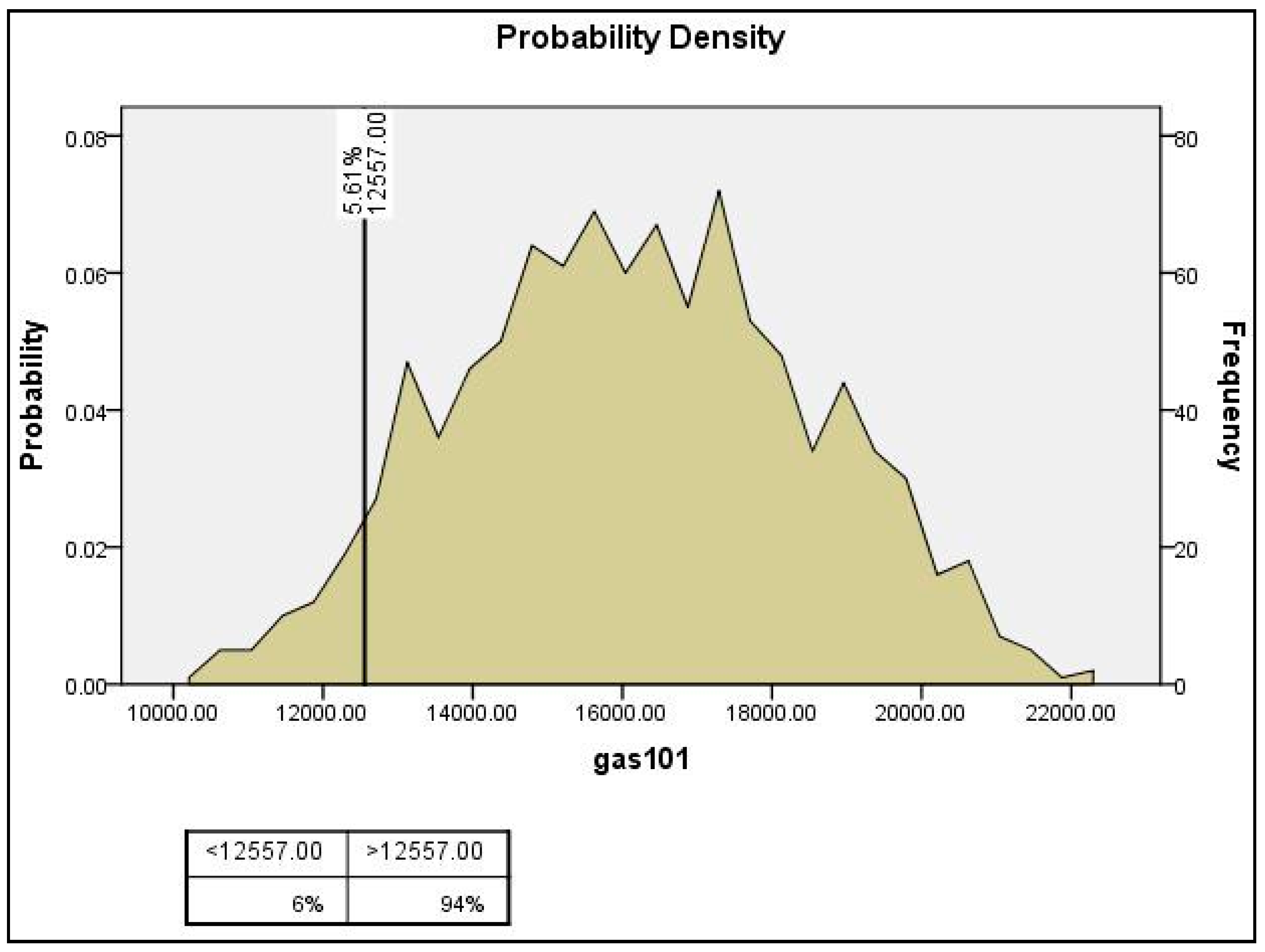
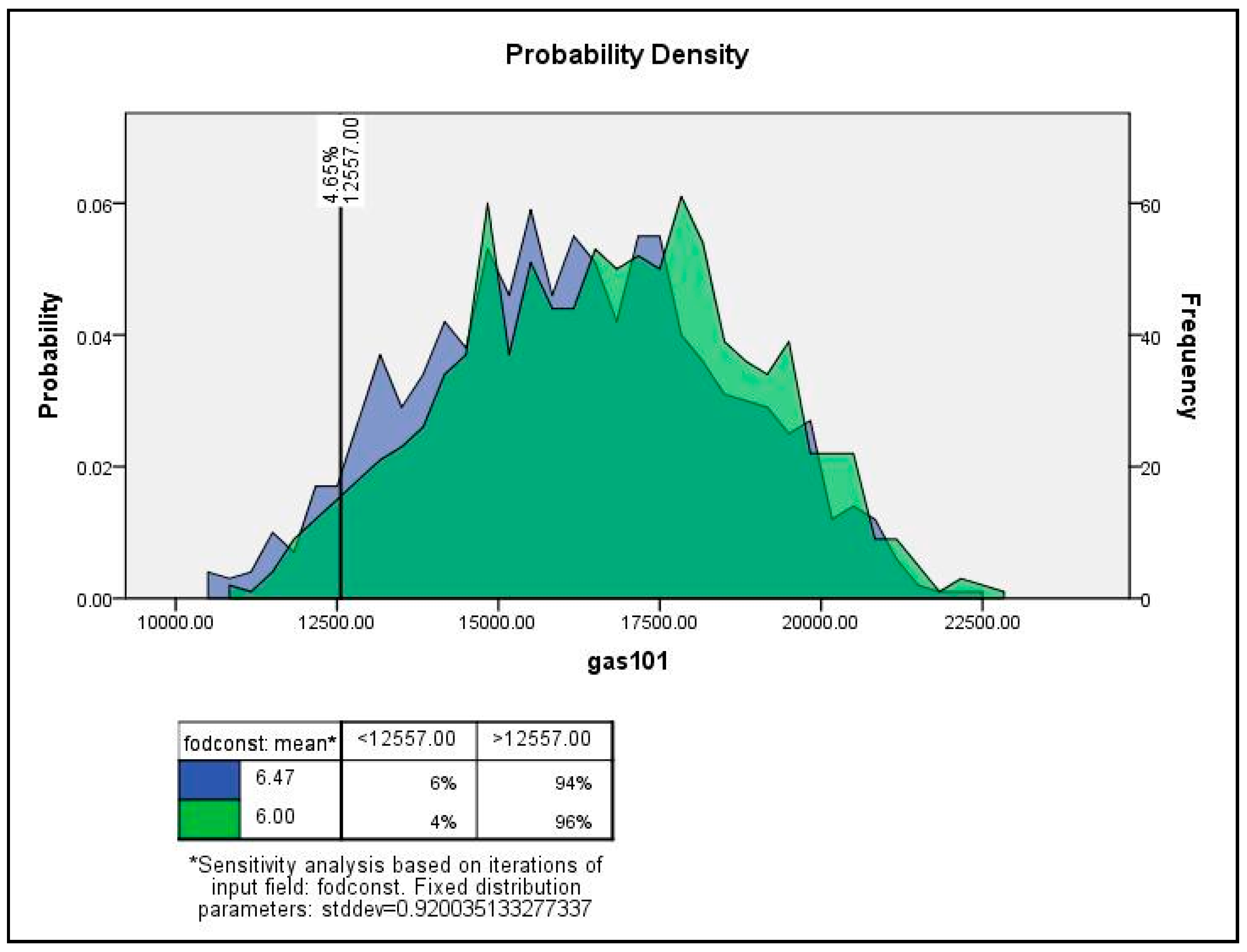
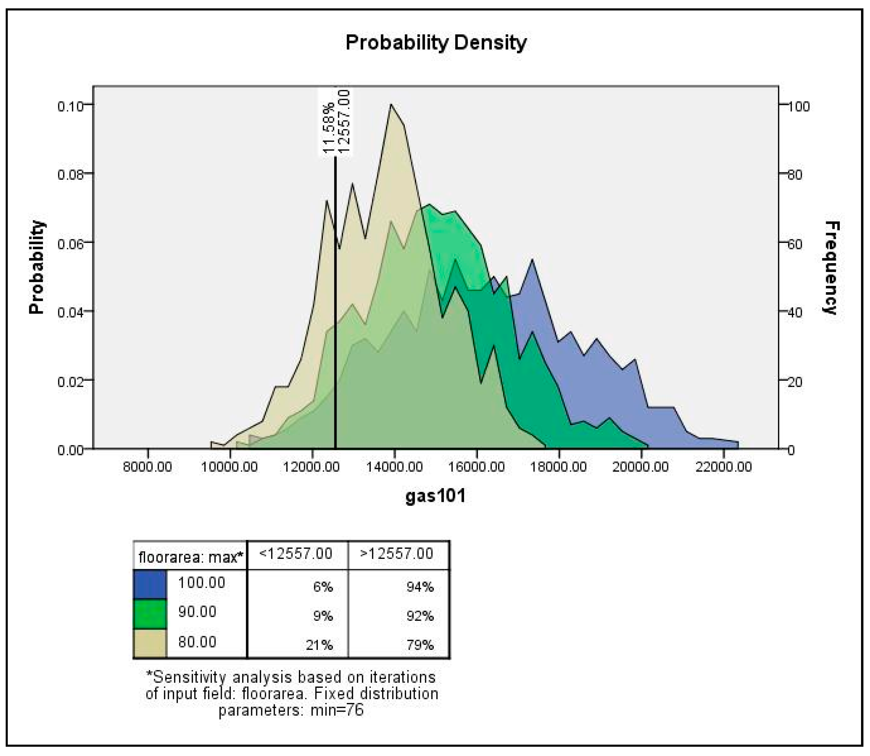
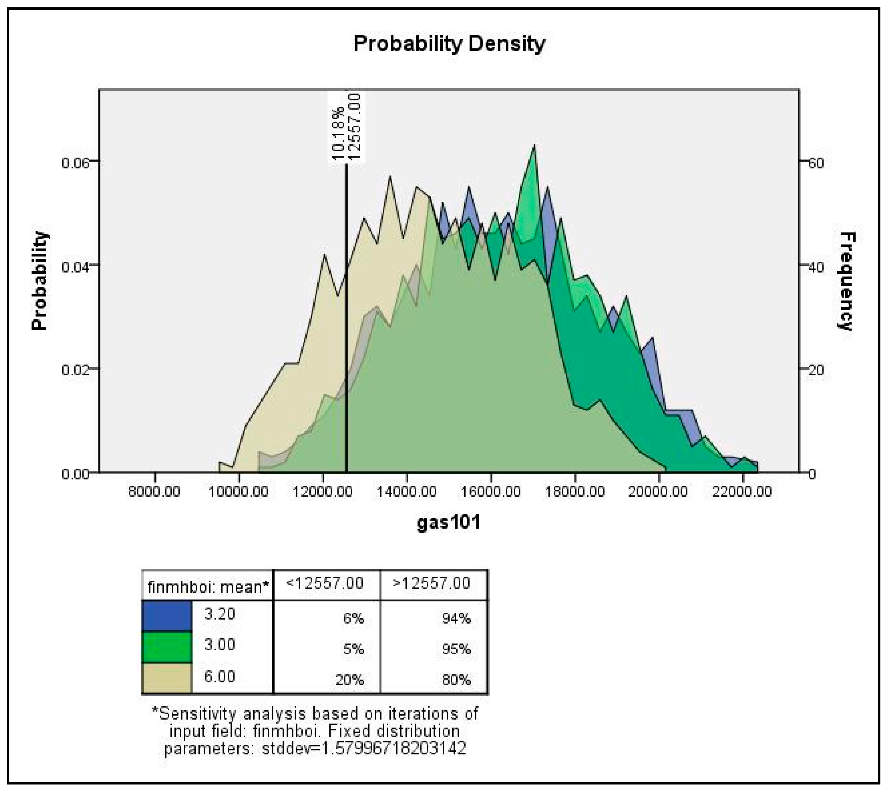
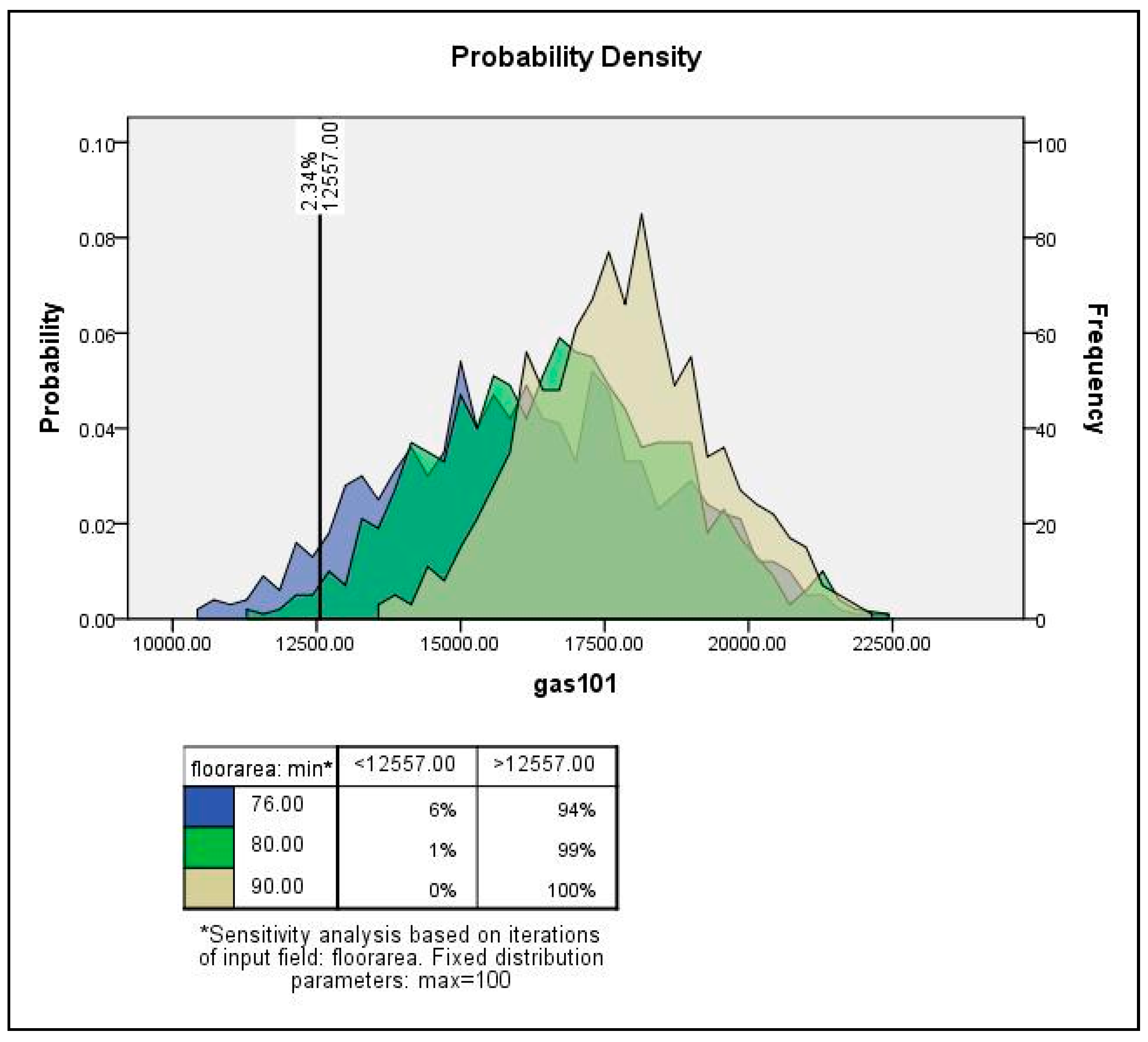
4.2. Monte Carlo Simulation and Sensitivity Analysis

Monte Carlo simulation is typically characterized by a large number of explanatory variables. This paper uses a parameter sensitivity analysis to quantify the effect of the explanatory variables (parameters) in the energy model output (annual heating gas consumption in dwellings). This information is then used to decide which explanatory variable should be optimized (or determined more accurately) through further survey or passed to a careful refined data process.

This section performs first a Monte Carlo by simulating the explanatory variables of the model (or the predictors) scoring the output of interest (in this research the DECC median value) as a base line. We then ‘tweak’ different predictor parameters of the model in a ‘what if’ and sensitivity analysis, i.e., using the NCRF estimated model sample results as a starting point and then change parameters from this base line. The Monte Carlo simulation results are analysed over a sample of 57 NCRF Castle bungalow dwellings age 1965 to 1962 and floor area 76 to 100 sqm.

The experimental framework uses the Monte Carlo simulation in the following roadmap: (i) a deterministic relation between annual heating gas consumption as the output (Y) and the predictors (X₁, ... X₆) are found (see fitted model Equation (2)); (ii) the probability density functions of X₁, ..., X₆ are fitted from sampled data along with the parameters (see Table 4); (iii) the correlations of existing inputs X₁, ..., X₆ are inputted to the Monte Carlo simulation; (iv) for each independent variable X₁, ..., X₆, 57 random numbers (57 Castle bungalows) are simulated that follow the probability density function properties of the previous step. As a result, a (57 rows × 6 columns) matrix of simulated independent data is then available; (v) the deterministic relation between Y and (X₁, ..., X₆) is applied to the previous matrix. As a result, 57 simulated values for Y are generated; and (vi) the resulting distribution for Y is finally examined for reasonable assumptions about the nature of uncertainty expected from the model and source data (see Section 2).

In summary, the NCRF sensitivity analysis is interested in what is the likelihood of achieving the 2009 DECC energy gas consumption (median value) for a new bungalow dwelling. The dependant variable is annual heating gas consumption and the predictors are: (i) usable floor area; (ii) dwelling type; (iii) construction date; (iv) cavity wall insulation; (v) primary heating fuel—type of system; and (vi) boiler group. The coefficients of the regression analysis are shown in

Table 5. Coefficients of the regression analysis ^a.

Model	Unstandardized Coefficients		Standardized Coefficients	Inferential Statistical t-Test	Significance Probabilty
	Beta Coefficients	Standard Error	Beta Coefficients
(Constant)	−2972.591	8527.128	-	−0.349	0.729
Floor area	249.533	68.817	0.452	3.626	0.001
Dwelling type	683.926	856.747	0.092	0.798	0.429
Dwelling age	−719.608	495.683	−0.186	−1.452	0.153
Cavity wall insulation	1379.358	789.407	0.195	1.747	0.087
Primary heating fuel	889.723	862.686	0.187	1.031	0.308
Boiler type	−1192.025	406.517	−0.530	−2.932	0.005

^a Coefficients considering the dependent variable the heating gas consumption.

.

Table 5 shows in the column ‘unstandardized coefficients’, the value of the constant, which is the intercept or the predictors (X₁, ..., X₆) if Y is ‘0’, in other words, if the predictors are ‘0’ the annual heating gas consumption is −2972.591. It also gives the predictor coefficients, i.e., the value that Y would change by if the corresponding predictors (X₁, ..., X₆) would change by 1 unit. Those values are 249.533, 683.926, −719.608, 1379.358, 889.723 and −1192.025, respectively, e.g., if the usable floor area goes up by 1, the annual heating gas consumption is predicted (see Equation (3)) to go up by 249.533. The standardized coefficient can be interpreted like the Pearson coefficient in bivariate associative analysis, i.e., a 0–1 scale with 1 being perfect correlate. Table 5 also shows the t-test and significance level (the probability of observing such an extreme value by chance).

$$\begin{array}{cc}\hfill Ga{s}_i=& -2972.591+249.533floorare{a}_i+683.926dwtype7x_i\hfill \\ & -719.608fodcons{t}_i+1379.358felcavf{f}_i+889.723Finchty{p}_i\hfill \\ & -1192.025finmhbo{i}_i\hfill \end{array}$$

(3)

Figure 5 shows the base line scenario analysis results for the probability of a new bungalow dwelling matching the median DECC value (see step vi in the roadmap above in this section). Figure 5 shows the likelihood (5.61%) of making the DECC median value in the Monte Carlo base line. The Statistical Package for the Social Sciences (SPSS) was used to create the probabilities density functions in this section and the output shows the NCRF estimates on the x axis. A peculiarity of SPSS is that it provides y axes showing the probability on the left and the frequency on the right. However, the shape of the curve and its position relative to the median DECC value is the key aspect of Figure 5.

Figure 5 shows the base line scenario analysis results for the probability of a new bungalow dwelling matching the median DECC value. There are two kinds of information in Figure 5: the dark-yellow graph, and the vertical line (with the associated table below the graph).

The vertical line represents the Median of the NEED values for heating gas consumption in bungalows in the study area. The dark yellow graph represents the heating gas consumption data for all bungalows in the study area from NCRF estimates. The small table below Figure 5 shows the percentage of the area below the curve to the left and right of the median DECC value. This means that based on our NCRM data, the likelihood of a new bungalow having an energy consumption less that the median value is 6% and greater than the DECC median value is 94%.

The black line on the top dark yellow graph is the probability density function (PDF) of the annual heating gas consumption (gas101) of the Castle bungalows. The PDF describes the relative likelihood for this random variable to take on the DECC median value. The horizontal axis shows the values of the annual heating gas consumption and the vertical axis shows the probability (on the left) and the relative frequency of occurrence (on the right). The likelihood (probability) of a new bungalow in Castle to have annual energy consumption less than 12,557 kWh (the DECC medium value) is the integral of the probability density function (is 0.0561 or 5.61%) up to 12,557 kWh. Other information in Figure 5 include: the probability of having an NCRF bungalow with a consumption less than 10,000 kWh is cero and the probability of having a bungalow with a consumption less than 22,000 kWh is almost one (100%).

In summary, the vertical line represents the annual energy consumption DECC (median value) (12,557 kWh) and the likelihood of a new bungalow having this value is 5.65% (almost 6%). In other words, the probability for a new bungalow having annual energy consumption less than 12,557 kWh is less than 5.65% and the probability for a new bungalow to have annual energy consumption more than 12,557 kWh is greater than 94.35%. The same type of representation is used in the ‘what if’ analysis.

The ‘what if’ analysis of changing parameters on the model and the effect on the likelihood of meeting the DECC median value are shown in Figure 6, Figure 7, Figure 8, Figure 9, Figure 10 and Figure 11. The sensitivity analysis modifies three predictors: Figure 6 is the year of construction estimator fitted by a normal probability distribution; Figure 7, Figure 8 and Figure 9, show changes in the usable floor area fitted by a uniform distribution, and Figure 10 and Figure 11 show changes boiler type fitted again by a normal probability distribution.

In Figure 6, Figure 7, Figure 8, Figure 9, Figure 10 and Figure 11 for all scenarios, the dark blue shows the base line, the green a small variation, the dark-yellow a medium variation and the purple colour a large variation of the estimator. The vertical line inside the graph shows the likelihood for a bungalow to have the DECC median value for the base scenario in the particular test.

In Figure 6, a decrease in the expected (mean) value of the year of construction of new bungalows drives the graph away from the DECC median value (decreases the likelihood to meet the median DECC value), i.e., a decrease in the year of construction increases the annual heating gas consumption, presumably as the older bungalows have inferior insulation. Even if they have improved insulation, it is unusual to retrofit underfloor insulation or the like and the building regulations were not as restrictive as current ones.

In Figure 7, an increase in the minimum value of the floor area (being a uniform distribution) decreases the likelihood of meeting the median DECC value. An increase in the minimum value floor area also increases the energy consumption (because only bigger bungalows remain in the sample) or decreases the availability of local bungalows with smaller areas. Note also that the likelihood of finding bungalows in the range of 90 to 100 sqm, in the North East of England (NEE) is zero.

In Figure 8, a decrease in the maximum value of the floor area increases the likelihood of meeting the median DECC value. This produces the opposite to Figure 7 as the bungalows that remain in the sample are of small area, so the annual heating gas consumption is small. Also, the graph seems to suggest that the representative bungalow in NEE is smaller than in the Castle bungalow sample (the likelihood is close to 20%).

In Figure 9, a decrease in the minimum value of floor area (or increasing the range) results in the probability density almost matching the median DECC value. An interesting case is when the minimum value is changed from 76 sqm (dark-blue) to 50 sqm (purple). In this case, the NCRF median annual heating gas consumption almost matches the median DECC value. This confirms the fact that the Castle bungalows (local area bungalows) are of bigger floor area than the NEE (regional bungalows).

In summary, the usable floor area is a very sensitive parameter. For bungalows, if the range of usable floor area is towards the higher end then the likelihood of matching the DECC median decreases. If the range is in the lower values then the likelihood increases of matching the DECC median. This seems to confirm that NEE bungalows are smaller than Castle and, in broad terms, the usable floor area is the most sensitive parameter in the sub-city areas. This confirms that local area characteristics differ from regional medians.

In Figure 10, there is an increase in the mean of the boiler type towards more inefficient boiler types, and in Figure 11, a decrease in the mean of the boiler type towards more efficient boilers. A change in the boiler type to a more efficient one increases the likelihood of reaching the median DECC value. This suggests that the Castle boilers are not efficient (or that there are opportunities to implement energy efficiency measures in terms of replacing the boiler with an efficient one in Castle bungalows) compared to the NEE median dwelling, i.e., local area characteristics are important in energy planning.

5. Summary and Discussion

This paper characterized (and quantified where possible) the uncertainty in creating the domestic energy estimates.

There are a considerable number of uncertainties in the model, input, refinement and validation. This paper has proposed a three dimensional taxonomy to characterize the uncertainty: in the source, the issues (and the sub-issues) causing the uncertainty and whether that issue is due to the lack of knowledge or is due to the inherent variability of the variable being described. In order to provide a human friendly understanding of uncertainty, a Concept Map was proposed which identified concrete terminal causes of uncertainty within the taxonomic framework. Understanding uncertainty in this way provides a possible framework for modellers, policy makers and data collectors to improve practice in key areas and reduce uncertainty.

A Monte Carlo type analysis was carried out to understand the sensitivity of key energy parameters. Although this has been carried out on only one sample of data, it provides compelling evidence that local area characteristics are important in energy modelling and that national and regional indices and values may not properly reflect the local conditions resulting in programmes and interventions that will be sub-optimal.

In addition, it seems there is potential for this type of analysis to investigate and corroborate interventions within geographical or building age/type bounds through developing what-if scenarios for particular interventions (e.g., it is more important to increase the efficiency of boilers in bungalows in Castle because their footprint is larger than the regional estimates).

The core idea of our framework is to learn about a system by simulating it with random sampling. That approach is powerful, flexible and very direct. It is the simplest way to solve a problem, and the only feasible way. In our paper, the emphasis is on drawing a picture to gain qualitative insight. Such visualization is a very common use of Monte Carlo simulation methods where sometimes the picture is the goal in itself.

Finally, in this research the emphasis was on two (in a way) separate streams. First, the emphasis was on getting policy makers to understand how it is possible to model a ‘what if’ question scenario, realizing that uncertainty has to be taken into account in the model estimates. Second, the identification of the policy makers’ and stakeholders’ needs is not an easy task, and sometimes this is a process of negotiation (and is not really written in a project call specification), recognizing that there is a high degree of politics involved. However, what is important is the quality assurance in the conceptualization, structure and validation of both the model and output data estimates so they can be trusted by the decision makers.

References

1. Eisenhower, B.; O’Neill, Z.; Fonoberov, V.A.; Mezić, I. Uncertainty and sensitivity decomposition of building energy models. J. Build. Perform. Simul. 2012, 5, 171–184. [Google Scholar] [CrossRef]
2. Grömping, U. Estimators of relative importance in linear regression based on variance decomposition. Am. Stat. 2007, 61, 139–147. [Google Scholar] [CrossRef]
3. Nguyen, A.-T.; Reiter, S. A performance comparison of sensitivity analysis methods for building energy models. Build. Simul. 2015, 8, 651–664. [Google Scholar] [CrossRef]
4. Summerfield, A.J.; Raslan, R.; Lowe, R.J.; Oreszczyn, T. (Eds.) How useful are building energy models for policy? A UK perspective. In Proceedings of the 12th Conference of International Building Performance Simulation Association, Sidney, Australia, 14–16 November 2011. [Google Scholar]
5. Rubin, D.B. Multiple imputation after 18+ years. J. Am. Stat. Assoc. 1996, 91, 473–489. [Google Scholar] [CrossRef]
6. Kessler, R.C. The Categorical versus dimensional assessment controversy in the sociology of mental illness. J. Health Soc. Behav. 2009, 43, 171–188. [Google Scholar] [CrossRef]
7. Calderón, C.; James, P.; Urquizo, J.; McLoughlin, A. A GIS domestic building framework to estimate energy end-use demand in UK sub-city areas. Energy Build. 2015, 96, 236–250. [Google Scholar] [CrossRef]
8. Calderón, C.; James, P.; Alderson, D.; McLoughlin, A.; Wagner, T. Data Availability and Repeatability for Urban Carbon Modelling: A CarbonRouteMap for Newcastle upon Tyne; Retrofit: Manchester, UK, 2012. [Google Scholar]
9. Hickman, J.; Baybutt, P.; Bell, B.; Carlson, D.; Conradi, L.; Denning, R. PRA Procedures Guide: A Guide to the Performance of Probabilistic Risk Assessments for Nuclear Power Plants: Chapters 9–13 and Appendices A–G (NUREG/CR-2300, Volume 2); Report No.: NRC FIN G-1004; Office of Nuclear Regulatory Research, U.S. Nuclear Regulatory Commission: Washington, DC, USA, 1983.
10. Macdonald, I.A.; Clarke, J.A. Applying uncertainty considerations to energy conservation equations. Energy Build. 2007, 39, 1019–1026. [Google Scholar] [CrossRef] [Green Version]
11. Chapman, J. Data accuracy and model reliability. In Proceedings of the BEPAC Conference, Canterbury, UK, 10–11 April 1991; pp. 10–19. [Google Scholar]
12. Unwin, S.; Moss, R.; Rice, J.M.S. Characterizing Uncertainty for Regional Climate Change Mitigation and Adaptation Decisions; Pacific Northwest National Laboratory, U.S. Department of Energy: Washington, DC, USA, 2011.
13. Lin, G.; Engel, D.W.; Eslinger, P.W. Survey and Evaluate Uncertainty Quantification Methodologies; Contract No.: PNNL-20914; Pacific Northwest National Laboratory (PNNL): Richland, WA, USA, 2012.
14. Han, P.K.J.; Klein, W.M.P.; Arora, N.K. Varieties of uncertainty in health care: A conceptual taxonomy. Med. Decis. Mak. 2011, 31, 828–838. [Google Scholar] [CrossRef] [PubMed]
15. Myung, I.J. The importance of complexity in model selection. J. Math. Psychol. 2000, 44, 190–204. [Google Scholar] [CrossRef] [PubMed]
16. Shapiro, S.C.; Eckroth, D. Encyclopedia of Artificial Intelligence; John Wiley & Sons, Inc.: New York, NY, USA, 1987. [Google Scholar]
17. Novak, J.D.; Cañas, A.J. The Theory Underlying Concept Maps and How to Construct Them; Florida Institute for Human and Machine Cognition: Pensacola, FL, USA, 2006. [Google Scholar]
18. Sowa, J.F. Semantic Networks. In Encyclopedia of Cognitive Science; John Wiley & Sons, Ltd.: New York, NY, USA, 2006. [Google Scholar]
19. Hughes, M.; Palmer, J.; Cheng, V.; Shipworth, D. Sensitivity and uncertainty analysis of England’s housing energy model. Build. Res. Inf. 2013, 41, 156–167. [Google Scholar] [CrossRef]
20. Cullen, A.; Frey, C. Probabilistic Techniques in Exposure Assessment: A Handbook for Dealing with Variability and Uncertainty in Models and Inputs; Springer: New York, NY, USA, 1999. [Google Scholar]
21. U.S. Food and Drug Administration. Guidance for Industry: Estimating Dietary Intake of Substances in Food. 2015. Available online: http://www.fda.gov/RegulatoryInformation/Guidances/ucm074725.htm#ftn50 (accessed on 14 August 2015).
22. Matthys, C.; Bilau, M.; Govaert, Y.; Moons, E.; De Henauw, S.; Willems, J.L. Risk assessment of dietary acrylamide intake in Flemish adolescents. Food Chem. Toxicol. 2005, 43, 271–278. [Google Scholar] [CrossRef] [PubMed]
23. Helton, J.C.; Johnson, J.D.; Sallaberry, C.J.; Storlie, C.B. Survey of sampling-based methods for uncertainty and sensitivity analysis. Reliab. Eng. Syst. Saf. 2006, 91, 1175–1209. [Google Scholar] [CrossRef]
24. Helton, J.C.; Johnson, J.D.; Oberkampf, W.L. An exploration of alternative approaches to the representation of uncertainty in model predictions. Reliab. Eng. Syst. Saf. 2004, 85, 39–71. [Google Scholar] [CrossRef]
25. Cooke, R.M. Experts in Uncertainty: Opinion and Subjective Probability in Science; Oxford University Press: New York, NY, USA, 1991; 330p. [Google Scholar]
26. Manache, G.; Melching, C.S. Identification of reliable regression- and correlation-based sensitivity measures for importance ranking of water-quality model parameters. Environ. Model. Softw. 2008, 23, 549–562. [Google Scholar] [CrossRef]
27. International Energy Agency (IEA). Sensitivity and Uncertainty—Annex 31: Energy-Related Environmental Impact of Buildings; IEA: Otawa, ON, Canada, 2004. [Google Scholar]
28. Boriah, S.; Chandola, V.; Kumar, V. Similarity Measures for Categorical Data: A Comparative Evaluation. In Proceedings of the SIAM Conference on Data Mining, Atlanta, GA, USA, 24–26 April 2008; Society for Industrial and Applied Mathematics: Philadelphia, PA, USA, 2008; pp. 243–254. [Google Scholar]
29. Jolliffe, I.T. Principal Component Analysis; Springer: New York, NY, USA, 2002; Available online: http://www.springer.com/us/book/9780387954424 (accessed on 20 September 2017).
30. Dougherty, C. Introduction to Econometrics, 3rd ed.; Oxford University Press Inc.: New York, NY, USA, 2007. [Google Scholar]
31. Silverman, B.W. Density estimation for statistics and data analysis. In Monographs on Statistics and Applied Probability; Chapman and Hall: London, UK, 1986. [Google Scholar]
32. Quinn, G.P.; Keough, M.J. Experimental Design and Data Analysis for Biologists. 2002. Available online: http://www.amazon.co.uk/Experimental-Design-Data-Analysis-Biologists/dp/0521009766 (accessed on 10 September 2017).
33. Hughes, M. A Guide to the Cambridge Housing Model; The Department of Energy & Climate Change (DECC): London, UK, 2011.
34. Saltelli, A.; Annoni, P. How to avoid a perfunctory sensitivity analysis. Environ. Model. Softw. 2010, 25, 1508–1517. [Google Scholar] [CrossRef]
35. Confalonieri, R.; Bellocchi, G.; Tarantola, S.; Acutis, M.; Donatelli, M.; Genovese, G. Sensitivity analysis of the rice model WARM in Europe: Exploring the effects of different locations, climates and methods of analysis on model sensitivity to crop parameters. Environ. Model. Softw. 2010, 25, 479–488. [Google Scholar] [CrossRef]
36. Ziehn, T.; Tomlin, A.S. GUI–HDMR—A software tool for global sensitivity analysis of complex models. Environ. Model. Softw. 2009, 24, 775–785. [Google Scholar] [CrossRef]
Figure 1. Uncertainty characterization [12].
Energies 10 01986 g001
Figure 2. NCRF outcome uncertainties.
Energies 10 01986 g002
Figure 3. NCRF model concept map.
Energies 10 01986 g003
Figure 4. Framework combining principal component regression and Monte Carlo Simulation.
Energies 10 01986 g004
Figure 5. Typical Castle bungalow age: 1965 to 1962 and floor area: 76 to 100 sqm.
Energies 10 01986 g005
Figure 6. ‘What if’ scenario sensitivity analysis decreasing the year of construction.
Energies 10 01986 g006
Figure 7. ‘What if’ scenario sensitivity analysis increasing the minimum usable floor area.
Energies 10 01986 g007
Figure 8. ‘What if’ scenario sensitivity analysis decreasing the maximum floor area.
Energies 10 01986 g008
Figure 9. ‘What if’ scenario sensitivity analysis decreasing the minimum floor area.
Energies 10 01986 g009
Figure 10. ‘What if’ scenario sensitivity analysis changing to an increasing inefficient boiler.
Energies 10 01986 g010
Figure 11. ‘What if’ scenario sensitivity analysis changing to an increasing efficient boiler.
Energies 10 01986 g011