Day-Ahead Wind Power Forecasting Using a Two-Stage Hybrid Modeling Approach Based on SCADA and Meteorological Information, and Evaluating the Impact of Input-Data Dependency on Forecasting Accuracy

Abstract

The power generated by wind generators is usually associated with uncertainties, due to the intermittency of wind speed and other weather variables. This creates a big challenge for transmission system operators (TSOs) and distribution system operators (DSOs) in terms of connecting, controlling and managing power networks with high-penetration wind energy. Hence, in these power networks, accurate wind power forecasts are essential for their reliable and efficient operation. They support TSOs and DSOs in enhancing the control and management of the power network. In this paper, a novel two-stage hybrid approach based on the combination of the Hilbert-Huang transform (HHT), genetic algorithm (GA) and artificial neural network (ANN) is proposed for day-ahead wind power forecasting. The approach is composed of two stages. The first stage utilizes numerical weather prediction (NWP) meteorological information to predict wind speed at the exact site of the wind farm. The second stage maps actual wind speed vs. power characteristics recorded by SCADA. Then, the wind speed forecast in the first stage for the future day is fed to the second stage to predict the future day’s wind power. Comparative selection of input-data parameter sets for the forecasting model and impact analysis of input-data dependency on forecasting accuracy have also been studied. The proposed approach achieves significant forecasting accuracy improvement compared with three other artificial intelligence-based forecasting approaches and a benchmark model using the smart persistence method.

1. Introduction

The deployment of renewable energy sources (RESs) such as wind power generation systems (WPGSs) has gained significant attention in many countries following the signing of the Kyoto agreement. This is because wind energy is easily accessible (i.e., is available everywhere), clean, zero-emission (i.e., environmentally friendly) and simple (i.e., has a less complex structure than conventional energy sources). This has been made possible by the recent advent of power electronic converters and control technologies. In spite of being considered to be a next-generation energy source, and its considerable ecological benefits, the intermittency and volatility of wind speed and other weather variables makes the output power of WPGS completely uncertain, in contrast to conventional energy resources. Due to this uncertainty, it can be difficult to connect large amounts of wind power into a power grid. Nevertheless, this hardship is not insurmountable. In order to increase the economic competence and popularity of wind power, and to decrease the consequences of power fluctuation resulting from over- or underestimation of generation, accurate forecasting of wind power is very important. An accurate forecasting system can assist TSOs, DSOs and power trading industries in making the right decisions on critical issues. From a smart-grid perspective, this can allow TSOs, DSOs, and dispatching schedulers to enhance the power grid control and management. Hence, accurate day-ahead (short-term) output power forecast of WPGS in large power grids or microgrids is very important for the efficient, economical, stable and sustainable operation of the power supply.

A number of techniques have been implemented recently to forecast wind power and speed. The current techniques can be categorized as statistical, physical, or time-series methods, according to the forecasting models they utilized [1]. Recently, researchers have utilized a combination of statistical and physical models to obtain an optimal strategy that is still valid for forecasting systems with longer horizons. In these strategies, the statistical model plays a supplementary role to the forecasting input data collected by physical methods.

Although two main kinds of technique have been explored for wind power forecasting (comprehensive assessments of these techniques are presented in [2,3]), as indicated earlier, the combination of statistical and physical methods is more frequently used than the others [4,5]. Additionally, many other spatial correlation approaches have been presented for short-term wind power forecasting, with the aim of achieving better forecasting accuracy [6]. On the other hand, over time and, with the advent of advanced computer programming languages, more sophisticated and intelligent techniques have been proposed for short-term wind power forecasting. For example, Artificial Neural Networks (ANNs) [7,8,9], ANNs with Gaussian process estimation and adaptive Bayesian learning [10], combinations of wavelet transform and ANNs [11], fuzzy logic methods in [5,12], Kalman filters [13], support vector machines [14], and adaptive neuro-fuzzy inference systems (ANFIS) [15] have all been proposed for wind power forecasting.

Among the references listed above, those wind power forecasting approaches based on artificial intelligence have shown improved forecasting accuracy compared to the others. Nevertheless, most of those approaches are based solely on the wind power time series data taken from SCADA (supervisory control and data acquisition) historical records of wind farms, and do not incorporate meteorological variables. Such techniques face serious challenges when there is data missing from the historical SCADA records used as the training input dataset, and are therefore unable to provide accurate forecasts.

Further investigating the available research studies in the area, new forecasting strategies and methods of input-output data treatments are still in demand, with the aim of improving wind power forecasting accuracy and reducing the uncertainty in wind power forecasting, while maintaining practically reasonable computation times. This target has led to two-stage techniques, consisting of hybrid models in each stage. These techniques make use of both statistical (WPGS SCADA records) and physical (NWP weather parameters) data sources to develop relatively accurate short-term wind power forecasting models. Specifically, two-stage hierarchical forecasting approaches based on ANFIS [16], a combination of PSO and ANNs (hybrid PSO-ANN) [17], and a combination of genetic algorithms (GA) and ANNs (hybrid GA-ANN) [18] have been implemented for short-term wind power forecasting, making use of historical SCADA records for wind speed and power, as well as NWP weather variables. The findings from these papers have shown improved forecasting accuracy; furthermore, the approaches are effective for wind farms with missing or skipped SCADA records, but only if there are reasonably good approximations of NWP meteorological variables available in the vicinity of the wind farm site. However, in these approaches, a comparative selection of other possible combinations of input parameter sets for the forecasting model have not been considered; additionally, the influences of input-data selection on forecasting accuracy have not been studied. Moreover, the details of the algorithms used for the optimization of the ANN connection weights and ANFIS membership function parameters have not been discussed, thus far.

Reference [16] employed historical SCADA records of wind speed and power, as well as NWP weather variables, to establish a hierarchical wind power forecasting model. A comparative selection of other possible combinations of input parameter sets for the model was been presented; however, the forecasting accuracy obtained was not sufficiently accurate, due to the ANFIS membership function training algorithm used in the paper. This could be improved by utilizing more global optimization algorithms.

References [17,18] also proposed double-stage hierarchical hybrid models for short-term wind power forecasting by making use of historical SCADA records of wind speed and power, and NWP weather variables. The forecasting accuracies obtained in these models are promising; nevertheless, there is still room to possibly improve their forecasting accuracy, and this could be achieved by adding some additional features and combining them with other algorithms.

In this paper, a novel and robust two-stage day-ahead wind power forecast modeling approach based on the combination of the Hilbert-Huang transform (HHT), GAs and artificial neural networks (ANN) is proposed. The proposed two-stage hybrid HHT-GA-ANN forecasting approach is compared with two-stage back propagation artificial neural network (BP-ANN), two-stage hybrid GA-ANN, and two-stage hybrid Wavelet-GA-ANN approaches to reveal its robustness with respect to computation time and forecasting accuracy. This paper is an extension of the conference paper in [18].

The major contributions of this paper are summarized below:

(1)

Present a novel and robust double stage hierarchical hybrid strategy for short-term wind power prediction taking into account both statistical (actual wind speed and power SCADA records) and physical (NWP meteorological variables: wind speed, wind direction, air pressure, air temperature and humidity) factors;

(2)

Enhance prediction accuracy with respect to the prediction accuracy levels obtained with three other artificial intelligence-based approaches, as well as in comparison to a benchmark model using the smart persistence method;

(3)

Provide a practical solution to prediction challenges for wind farms having missed or jumped SCADA records of wind speed and power.

The paper is organized as follows. Section 2 describes the proposed two-stage forecasting approach. Section 3 provides the description and preprocessing of the input dataset of the forecasting model. The architecture of the HHT-GA-ANN forecasting system, along with a brief overview of the working principles of HHT, GA and ANN, is presented in Section 4. Section 5 provides different metrics used to evaluate prediction accuracy. The numerical findings and forecasting results for the real case-study wind farm being examined are provided in Section 6. The conclusions of the paper are outlined in Section 7.

2. Proposed Day-Ahead Wind Power Forecasting Strategy

The proposed forecasting strategy is based on the combination of HHT, GA and ANN. HHT is utilized to decompose the NWP meteorological variables, SCADA wind speed and power series into a set of improved-characteristic subseries. The decomposed historical values of these subseries are used to train the ANN. The future subseries values of NWP meteorological variables are then used to forecast the future wind power subseries using the ANN. The GA is utilized to optimize the parameters of the connection weights between the neurons of the ANN to achieve a higher forecasting accuracy and improved performance. Finally, the forecasted future wind power series is reconstructed by applying the inverse HHT.

The proposed strategy has two HHT-GA-NN stages, shown in Figure 1. In the initial stage, HHT-GA-ANN is implemented to forecast wind speed at the exact wind turbine hub height on the wind farm installation site. In this stage, in order to train the ANN, historical NWP meteorological variables (wind speed, wind direction, air pressure, air temperature and humidity) are used as inputs and historical actual wind speed SCADA measurement records are used as the target output. In the second stage, HHT-GA-ANN is modeled to map the wind speed versus power characteristics solely based on actual historical SCADA wind farm records. Subsequently, the wind speed predicted by the HHT-GA-ANN model in the initial stage is fed to the HHT-GA-ANN model developed (trained) in the second stage in order to forecast the future output power of the wind farm.

3. Data Description and Preprocessing

3.1. Wind Farm SCADA System

SCADA, as the main data acquisition and control system for wind farms, is a critical component, and plays a key role in wind power forecasting systems. Operating a real-time SCADA system offers the operator the ability to supervise the wind farm by managing all of the system parameters online. This possibility, for the real wind farm studied in this paper, allowed the operator to set appropriate actions in critical situations on the basis of a ten-minute and/or one-hour record of the wind farm information. In addition, this SCADA management system provides comprehensive records of the wind farm converters’ status and power outputs, as along with the operational availability of the wind turbines, which then act as the basis for short-term wind power forecasting.

In this paper, SCADA wind power data was a vector containing the historical SCADA wind power records for one year, with a time-step of 10 min (52,560 measured power values). The SCADA power record for the wind farm was based on the Beijing time zone (BJT), and wind farm in the case study was located in Beijing, China.

3.2. NWP Model and Meteorological Variables

Meteorological data has a considerable impact on wind power prediction. There are a number of methods that can be used to obtain meteorological data: observation/measurement, data mining, and NWP models. The most accurate and reliable technique for obtaining meteorological data is through measurement at the desired site, but this is not always feasible, and the data is not always accessible. Data mining techniques are relatively flexible, yet their capability to downscale the meteorological data is inadequate. NWP meteorological models employ equations based on physical conservation of energy, and this allows a more reasonable downscaling of the weather data. NWP models with higher resolutions or smaller coverage areas play a critical role in the improvement of wind power forecasting accuracy.

In recent times, with regard to the availability of sophisticated computational systems, a great deal of wind power forecasting research has been carried out utilizing weather data from NWP models. These research studies have used various NWP models, such as COSMO, WRF, RAMS and MM5 [19,20,21,22]. Moreover, several extrapolation methods, such as logarithmic law and wind shear power law, have been presented by researchers as offering accurate meteorological information at the desired wind turbine hub height using weather data gathered at 10 m above the ground [23]. In this study, the forecasting system uses meteorological predictions of a specific NWP model, called the WRF model, obtained in the vicinity of the wind farm installation site.

This WRF model is initialized at about 00:00 and 12:00 by Crontab task each day. Its domain size is 76 × 76 latitude-longitude grids, each with 3 km horizontal and vertical resolutions. The boundary conditions are set using GFS global forecasts. The WRF forecast horizon is 102 h ahead, with a 15 min time interval. The forecasts are issued twice a day, before 6:00 and 18:00. Each forecast issue is valid for about 90 h.

In this paper, the WRF meteorological data is a matrix with a set of values consisting of meteorological variables, arranged in 5 columns. Each column of the matrix is associated with one meteorological variable, and contains the variable’s historical values for one year with a time-step of 15 min (35,040 historical values). Columns 1–5 represent the wind speed, wind direction, air pressure, air temperature, and humidity values, respectively. In total, this matrix has 175,200 historical weather variable values. The WRF meteorological data record is based on Greenwich Mean Time (GMT), which is eight hours behind BJT.

3.3. Data Preprocessing

In the data preprocessing stage, the input dataset is processed to further simplified forms before the HHT-decomposition and ANN-training stages are started:

(1)

Both the SCADA wind power and NWP meteorological data are converted to hourly-average data with one-hour time-step to match the time interval of the two data sources;

$$x_{hourly}\left(t\right)=\frac{{\displaystyle \sum _{t=1}^6{x}_{10-\min }\left(t\right)}}{6}, \mathrm{for} \mathrm{the} \mathrm{SCADA} \mathrm{data}$$

(1)

$$x_{hourly}\left(t\right)=\frac{{\displaystyle \sum _{t=1}^4{x}_{15-\min }\left(t\right)}}{4}, \mathrm{for} \mathrm{the} \mathrm{WRF} \mathrm{data}$$

(2)

where, x_10-min(t), x_15-min(t) and x_hourly(t) are the 10-min interval SCADA power data value, the 15-min interval WRF meteorological data value, and the corresponding hourly-average data value, respectively.

(2)

The NWP meteorological data records are shifted to BJT to match with the time zone of the SCADA power data record;

$$x_{BJT}\left(t\right)=x_{GMT}\left(t+8\right)$$

(3)

where, x_BJT(t) and x_GMT(t) are the hourly average values of the meteorological data in BJT and GMT, respectively.

(3)

Missed or skipped data from either source is substituted by equivalent data using the following jumped data-filling technique.

$$x_i={\lambda }_1{x}_{i-24}+{\lambda }_2{x}_{i+24}$$

(4)

where x_i represents the data value of the ith sampling point, and λ₁ and λ₂ are the weights for calculation (taken as 0.5 in this paper). x_i−24 and x_i+24 represent the data values at the same time on the previous day and the next day, respectively.

4. Proposed Configuration for the Hybrid HHT-GA-ANN Model

4.1. Hilbert-Huang Transform (HHT)

The magnitude of the generated power data acquired from wind generation systems changes in each time instant. Identification of the wind generation system and the nonstationary and nonlinear wind data condition requires the decomposition of the original data into different subseries components. The HHT decomposes the NWP meteorological and SCADA data series into a set of subseries. These subseries offer better performance characteristics than the original NWP meteorological and SCADA data series, and hence they can be used to forecast wind power more accurately. The reason for the better performance characteristics of the subseries is the high-accuracy signal decomposition ability of the HHT. Using the HHT, time localization of frequency appearance of the original data is performed in order to determine the instantaneous frequency of the time series data.

The instantaneous frequency can be determined using the Hilbert transform (HT) [24]. For the mono-component time series function f(t), HT is defined by:

$$y\left(t\right)=\frac{1}{\mathsf{\pi }}{\displaystyle \underset{-\infty }{\overset{\infty }{\int }}\frac{f\left(\tau \right)}{t-\tau }}d\tau$$

(5)

where, f(t) and y(t) denote the complex conjugate pair which defines the analytical time series function z(t) as:

$$z\left(t\right)=f\left(t\right)+jy\left(t\right)$$

(6)

Equation (6) can be expressed in a polar coordinate system as:

$$z\left(t\right)=a\left(t\right)e^{j\theta \left(t\right)}$$

(7)

where,

$$\begin{array}{l}a\left(t\right)=\sqrt{f{\left(t\right)}^2+y{\left(t\right)}^2}\\ \theta \left(t\right)=\arctan \left(\frac{y\left(t\right)}{f\left(t\right)}\right)\end{array}$$

(8)

Here, a(t) and θ(t) denote the instantaneous magnitude and phase of the analytical time series function z(t). a(t) and θ(t) provide the best local fit of a magnitude- and phase-varying trigonometric function to the f(t). The instantaneous frequency ω(t) can be derived from the instantaneous phase as:

$$\omega \left(t\right)=\frac{d\theta \left(t\right)}{dt}=\frac{\dot{y}\left(t\right)f\left(t\right)-y\left(t\right)\dot{f}\left(t\right)}{f^2\left(t\right)+y^2\left(t\right)}$$

(9)

The instantaneous frequency ω(t) is practically sensible only if θ(t) is a mono-component function (a mono-component function is a symmetrical or purely oscillatory function that oscillates around the zero-mean value [24]). Because θ(t) is obtained from f(t), f(t) should also be mono-component function. Nevertheless, most real-world time series functions, and especially those obtained from NWP meteorological forecasts and wind farm SCADA records, are not mono-component. Huang [24] has presented the Empirical Mode Decomposition (EMD) method in order to decompose a multi-component time series function into a mono-component subseries basis. With EMD, the original function is described by a sum of Intrinsic Mode Functions (IMFs) that are analogous to the harmonic function basis in Fourier transform (FT) or the approximations and details in Wavelet transform (WT). IMFs are mono-component functions that should meet the following criteria: (1) the number of zero-crossings and the number of extrema must be equal or differ, at maximum, by one; (2) the average value of the envelopes determined by local maxima and minima must be equal to zero at every point.

Hence, based on the assumption that any data consists of various simple IMFs, the EMD algorithm is developed to decompose a time series function (data or signal) into subseries functions, IMFs. IMFs are obtained from the original signal using a sifting procedure. In this procedure, lower and upper envelops are established by placing a cubic spline through the local minima and maxima. The mean of the envelops m₁ is subtracted from the function f(t) to get the first component h₁. Ideally, h₁ is an IMF, but practically this seldom happens. In order to generate an IMF, the sifting procedure is consecutively applied k times to h_i, until an IMF is obtained:

$$h_{1k}=h_{1\left(k-1\right)}-m_{1k}$$

(10)

The sifting procedure terminates when the standard deviation between two successive results is smaller than a given minimum value. The first IMF, which holds information concerning the highest frequency, is given by:

$$c_1=h_{1k}$$

(11)

Then, c₁ is subtracted from the initial time series function, and the residue r₁, which carries information regarding the lower frequency components (f(t) is multi-component function), is given by:

$$r_1=f\left(t\right)-c_1$$

(12)

In the EMD algorithm, r₁ is taken as the starting signal and the process repeats—c₂ is computed, etc., n times until one of the following criteria is met: (1) r_n or c_n has small energy; or (2) r_n is a monotonic signal. Applying the abovementioned procedure, the original time series function f(t) is decomposed as:

$$f\left(t\right)={\displaystyle \sum _{i=1}^n{c}_i}+r_n$$

(13)

Every IMF (c_i) is subject to HT using Equation (9) to calculate instantaneous frequencies. As f(t) is a multi-component function, it has more than one instantaneous frequency. Hence, the decomposition of the function f(t) using HHT [24] has the form below:

$$f\left(t\right)=\mathrm{Re}\left({\displaystyle \sum _{i=1}^n{a}_i\left(t\right)}\exp \left(j{\displaystyle \int {\omega }_i\left(t\right)dt}\right)\right)$$

(14)

where, the magnitude a_i(t) and the frequency ω_i(t) are instantaneous or time-variant. The Huang EMD preprocessor-based Hilbert transform, represented by Equation (14), is known as the Hilbert-Huang transform (HHT).

Hence, HHT decomposes the original signal into data driven basis oscillatory functions. Based on Equations (9), (13) and (14), it can be concluded that the HHT gives a complete, adaptive and approximately orthogonal subseries representation of the original time series signal. The frequency and time resolutions of the HHT are as large as the sampling rate permits.

One of the limitations of the EMD algorithm is that it produces unwanted (nonexistent) components at low frequencies [25]. To circumvent this, the cross-correlation μ_i of c_i with the initial time series signal f(t) is checked [25]. Only the IMFs with cross-correlation μ_i greater than a prespecified minimum value λ are taken as real IMFs. All the other IMFs are considered to be pseudo-components, and are summed to the residual r_n. This version of the HHT transform is denoted the Improved HHT transform, and shows a considerably enhanced performance at low frequencies as well.

On the other hand, FT decomposes a time series signal into predetermined simple harmonic functions (fixed resolution in time and frequency) [24]. The WT decomposition subseries representation of a signal also consists of an a priori, predefined set of approximations and details (wavelet is selected first) [26]. That is, neither the FT nor WT are able to show the instantaneous frequency and intrinsic behavior of a signal [27]. However, the HHT is able to determine the instantaneous frequency with high accuracy, and hence its decomposition is more accurate and representative. Thus, the HHT transform is chosen for the proposed day-ahead wind power forecasting model due to its having the highest accuracy for extracting detailed features of the NWP meteorological and wind farm SCADA data. That is, in this paper, the instantaneous magnitudes of the modal basis functions (IMFs) of the HHT transform (of the NWP meteorological and wind farm SCADA data) are employed as input variables of the GA-ANN wind power forecasting model.

The EMD algorithm is summarized in Algorithm 1.

Algorithm 1. The Improved HHT transform EMD algorithm

(1) Initialize: r0 = f(t), and i = 1 (2) Extract the ith IMF, IMFi (a) Initialize: hi(k−1) = ri, k = 1 (b) Extract the local minima and maxima of hi(k−1) (c) Interpolate the local minima and maxima using cubic spline technique to form lower and upper envelopes of hi(k−1) (d) Compute the mean mi(k−1) of the lower and upper envelopes of hi(k−1) (e) Let hik = hi(k−1) − mi(k−1) (f) Check whether hik meets the IMF conditions (g) If hik is an IMF then set IMFi = hik, else go to step (b) with k = k + 1 (3) Check cross-correlation μi of IMFi with f(t) (a) if μi ≥ λ then keep the ith IMFi, else eliminate the ith IMFi and add it to the residue ri, and then go to step (2) (4) Define: ri+1 = ri − IMFi If ri+1 still has at least two extrema then go to step (2), else the decomposition process is completed and ri+1 is the residue of the original time series signal

4.2. Genetic Algorithm (GA)

The majority of field-oriented engineering problems are expressed by mixed continuous-discrete, and discontinuous and con-convex design variables. Conventional nonlinear optimization methods are computationally expensive, inefficient, and generally result in a relatively optimal solution very close to the initial point, when applied to solving these types of engineering problems.

Genetic algorithms (GAs) are more appropriate for solving such problems, as they are capable of discovering the global best solution with a high degree of probability over a wide solution space. GAs were first proposed thoroughly by Holland [28]. The basic idea of GAs is based on the concept of biological evolution, and detailed working principles are described in the work of Rechenberg [29].

GAs were inspired by Darwin’s principle of survival of the fittest. The algorithm relies on the principle of genetics and natural selection. The basic elements of natural genetics—reproduction, crossover, and mutation—are employed in the genetic search process to produce better solutions and new offspring over generations.

GAs are different from conventional standard optimization methods by virtue of the aspects listed below [30]:

• A population of initial solutions, instead of a single solution, is utilized to start the solution-search process, hence GAs are less likely to get trapped at local solution-like points.
• GAs do not employ objective function derivatives, only the values of the objective function are employed in the search process.
• The GA design variables are coded as binary strings like chromosomes in natural genetics. Hence, the search mechanism is naturally fitted for solving integer and discrete programming problems. The length of the strings can also be adjusted for any required resolution in the context of continuous design variables.
• In each new generation, new string sets (offspring) are generated by making use of probabilistic transition principles, not deterministic principles.

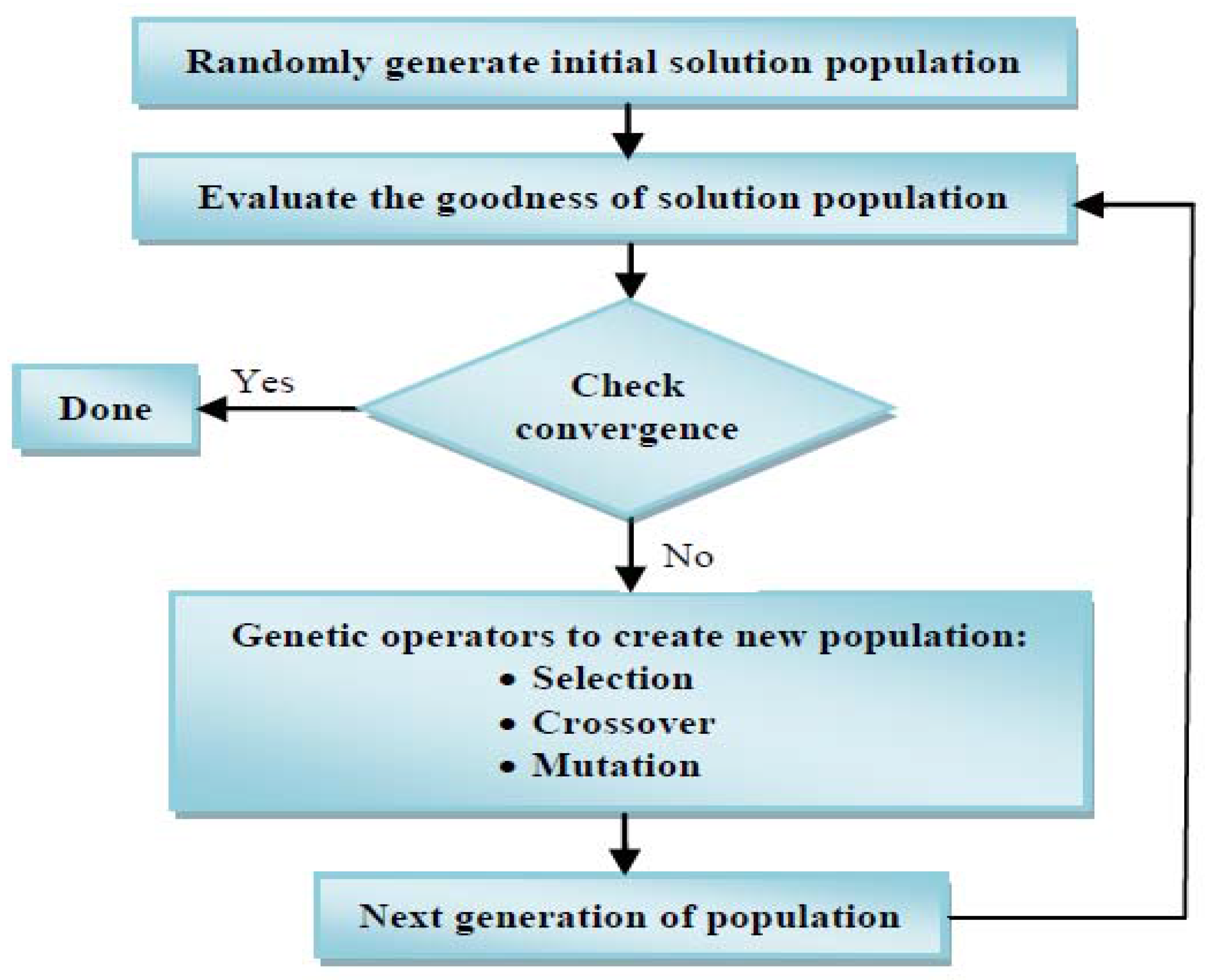
Figure 2 shows a flowchart diagram of GA.

As shown in Figure 2, the GA solution for an optimization problem starts with a population of random initial guess points (strings) representing a population of initial design vectors. The GA population size (n) is normally fixed. Each design vector (or string) is computed to determine its fitness value. A new population set is produced with the aid of the three GA operators: reproduction, crossover, and mutation. The newly generated population is also further evaluated to determine its associated fitness value, and then checked for the process convergence. One cycle of operator performance (reproduction, crossover, and mutation) and the evaluation of the associated fitness value is said to be one generation in GA. If the convergence metric is not satisfied, the population is iteratively performed again by the three operators, and the newly generated population is evaluated for the fitness value. This process continues through several generations until the convergence metric is met and the search process is over [30].

4.3. Artificial Neural Network (ANN)

ANN is an effective data-modeling mechanism that is capable of capturing and approximating the complex input/output relationships of datasets. It is a data processing model that was inspired by the mechanism by which human biological nervous systems, like the brain, manipulate information. The key feature of this model is its novel structure for information processing. The ANN model is composed of several data-processing elements (neurons) arranged in different layers of input, hidden, and output neurons. These neurons are tightly interconnected via some weighted connections, and all operate in unison to solve some specific data-modeling problem [31,32].

ANNs, like humans, learn things by example/experience. An ANN can be configured for a desired data processing application, such as data classification, pattern recognition, prediction, data fitting, through a learning/training process. Learning in biological systems is achieved through fine adjustments of the synaptic connections between neurons. In fact, this is true for ANNs as well. For the validation process, as well, ANN mimics the human brain, which offers proof of the existence of several ANNs that are effective at perceptual, cognitive, and control tasks at which humans are very successful.

In ANN modeling, the number of neurons in the hidden layer should be carefully selected. However, there is no explicit method to optimally size the hidden layer. In this paper, the size of the hidden layer was decided experimentally by a trial and error procedure. Different structures with different hidden layer sizes were investigated, and the best ANN structure was chosen based on root mean squared error (RMSE) criteria.

The ANN structure chosen in this paper is of the multi-layer feedforward (MLFF) type, shown in Figure 3, with parameters defined in

Table 1. Parameters of ANN.

Parameter	Value
Type	Multi-layer feedforward
Number of hidden layers	1
Number of hidden neurons	15
Hidden layer activation fn.	Hyperbolic tangent sigmoid (tansig)
Number of output layers	1
Number of output neurons	1
Output layer activation fn.	Pure linear (purelin)
Learning Rate	0.01
Number of epochs	1000
Learning goal/error	1.0 × 10−3

.

An illustrative representation of a multi-layer feedforward ANN is shown in Figure 3.

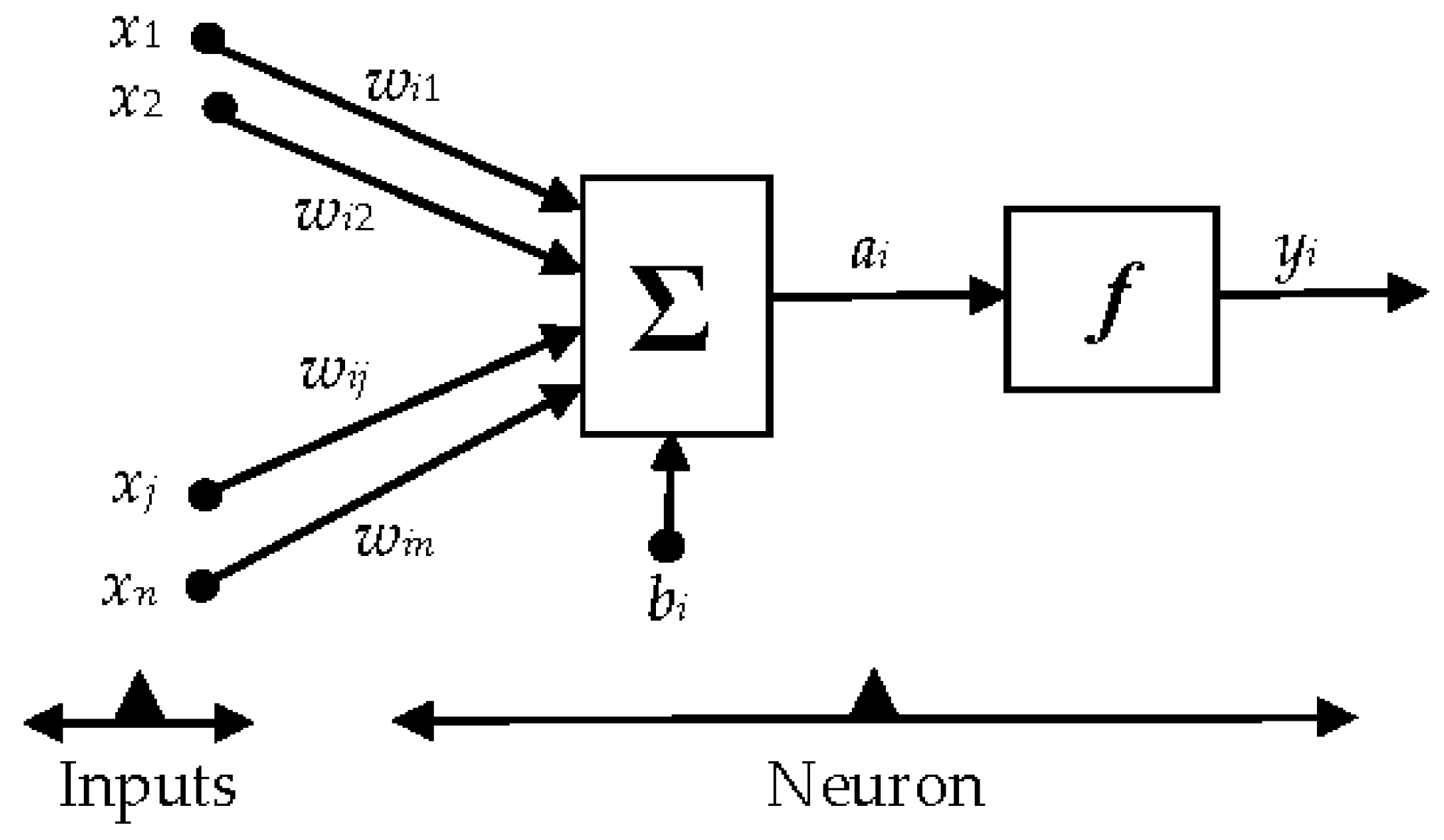
A descriptive representation indicating the mathematical model of a single neuron, ith neuron, of an ANN is also shown in Figure 4.

The mathematical relationship between the ANN inputs x_i and output y_i is given by:

$$y_i=f_i\left({\displaystyle \sum _{j=1}^n{w}_{ij}}·x_j+b_i\right)$$

(15)

where, x_j is the jth input to the ith neuron/node; y_i is the output of the ith node; w_ij is the connection weight between the neurons; b_i is the bias term of a neuron; and f_i is called the activation function of a neuron. The activation function plays a key role in the ANN training process, and determines the characteristics of the ANN.

Basically, MLFF ANN is a Back-Propagation (BP) algorithm-based network whose connection weight parameters are tuned with a BP algorithm based on some collection of input-output data. This allows the ANN network to learn. BP carries out a gradient descent within the solution’s vector space towards a global minimum value along the steepest vector of the error surface.

Though BP learning algorithms are fast, they can be trapped by local minima and are thus unable to attain global minima.

To overcome the BP algorithm difficulties, in this paper, the ANN in each stage of the forecasting model employs the GA optimization technique to optimally tune the weight parameters between neurons. The GA optimization method has the advantages of computational simplicity for a prespecified size of ANN structure. In this study, the ANN weight parameters are formed as variables of the GA, and the mean squared error is used as the objective cost function in GA. The objective of proposed approach is to achieve a minimum value for this cost function. This process continues until the forecast error reaches a desired value.

4.4. Proposed Two-Stage Hybrid Forecasting Model

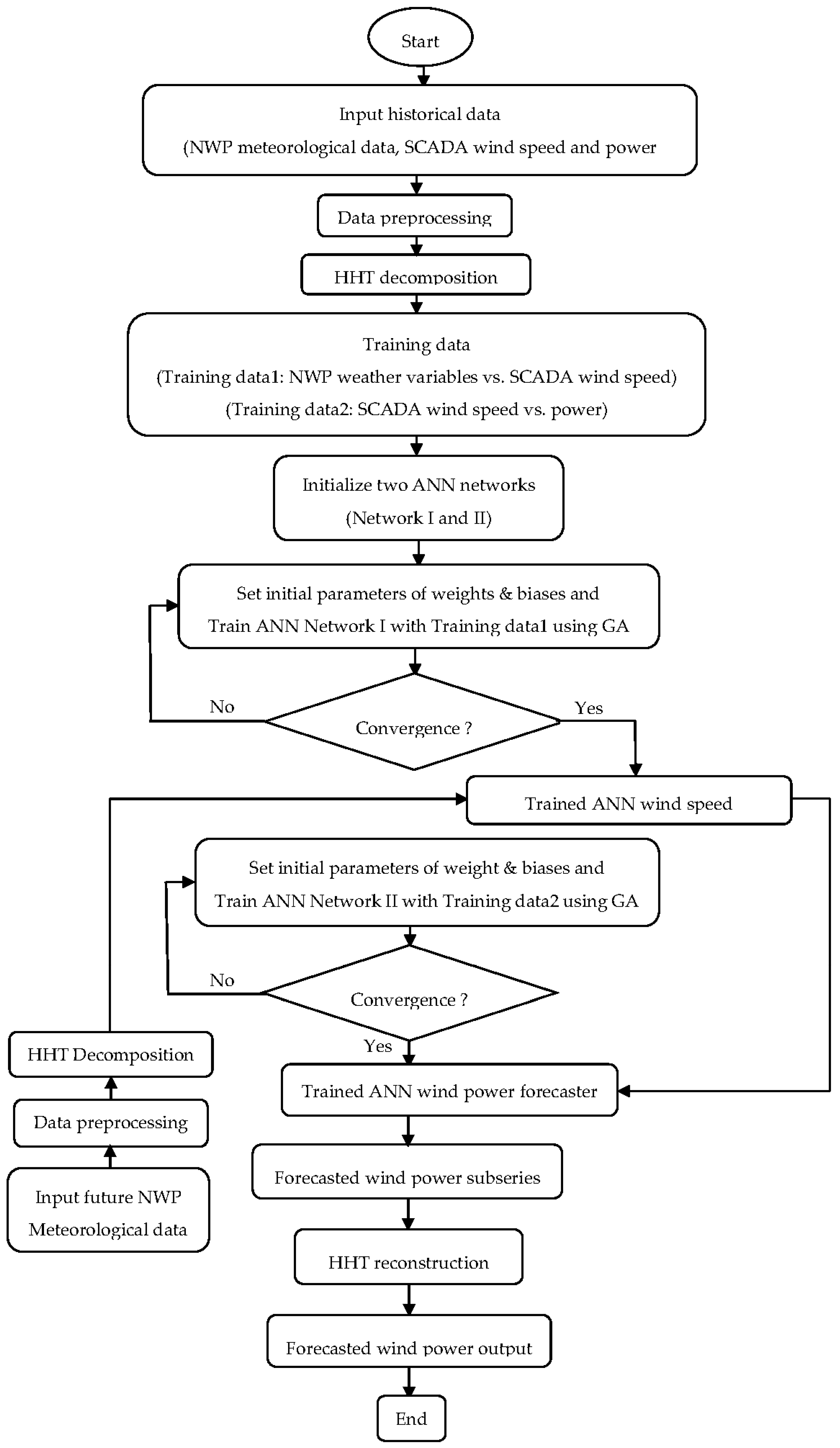
The two-stage hybrid algorithm used to realize the proposed wind power forecasting approach is presented step-by-step in Figure 5.

As shown in Figure 5, HHT techniques are implemented for data decomposition and reconstruction purposes, respectively, in the first and last stages.

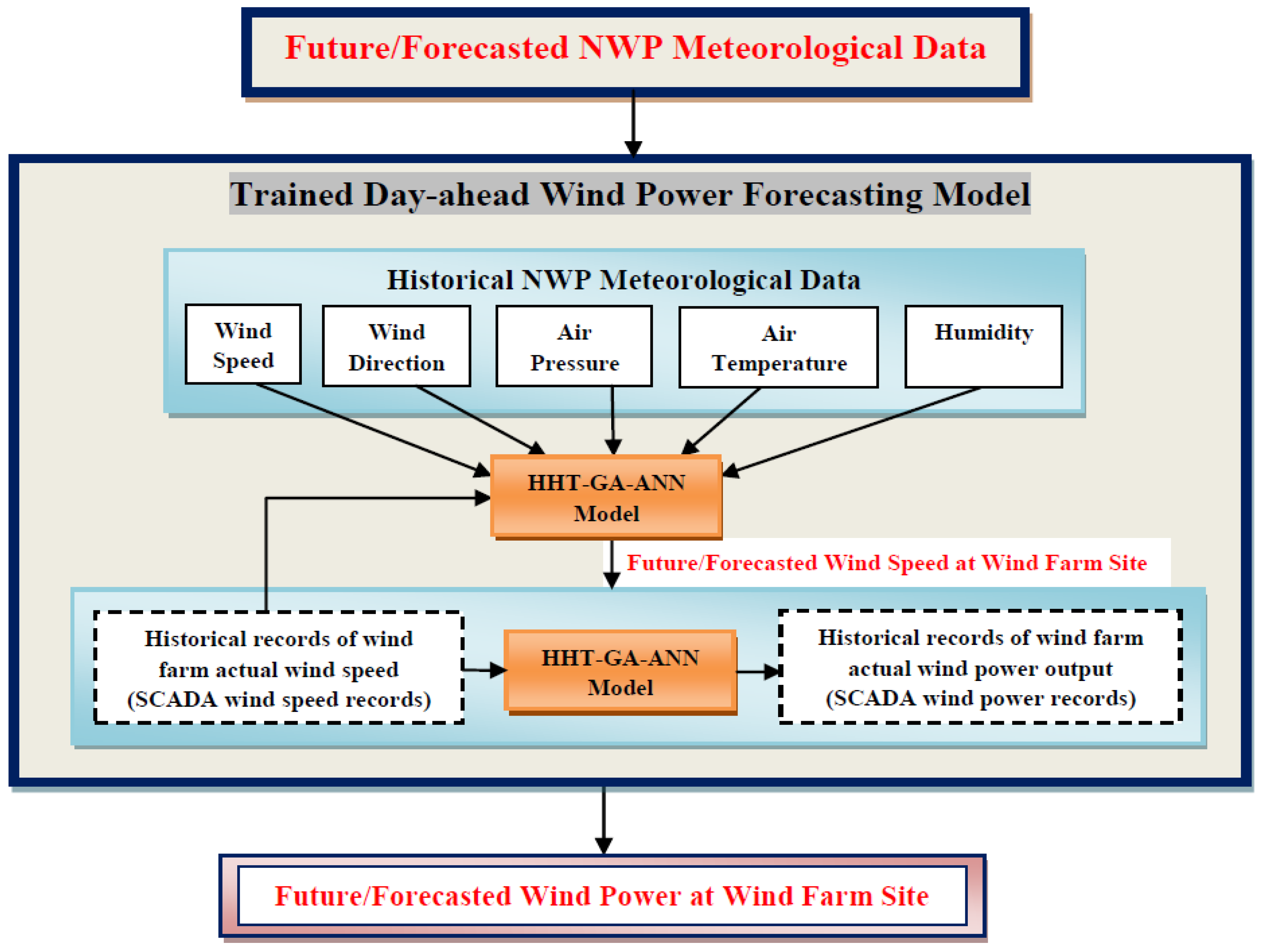
Each of the original series of NWP meteorological variables (wind speed, wind direction, air pressure, air temperature and humidity) and actual SCADA wind speed are decomposed separately into modal basis functions by the HHT, and each set of subseries is used separately to train the ANN Network I in the first stage, as shown in Figure 5. This is implemented to obtain a trained model, enabling the forecasting of wind speed at the exact wind turbine hub height on the wind farm installation site from regional forecasts of NWP meteorological variables. Similarly, the original series of actual SCADA wind power is decomposed into basis functions by the HHT. Each subseries, together with the actual SCADA wind speed subseries, is used separately to train the ANN Network II in the second stage, as shown in Figure 5. This is implemented to obtain a trained model, enabling one to map the wind turbine speed-power curve characteristics exactly, based on actual wind farm SCADA measurement records.

Then, the wind speed subseries predicted by the GA-ANN model in the initial stage is fed to the developed (trained) GA-ANN model in the second stage in order to forecast the future output power subseries of the wind farm.

Finally, the future power subseries signals are recombined in the final stage to form the final forecasted wind power series of the wind farm.

The parameters associated with the ANN and GA in the paper are defined in Table 1 and

Table 2. Parameters of GA.

Parameter	Value
Population size	100
Number of generations	1000
Selection method	Roulette wheel
Crossover type	Scattered
Crossover rate	0.8
Mutation type	Constraint dependent
Mutation rate	0.001

, respectively.

5. Forecasting Accuracy Evaluation Metrics

In order to estimate the accuracy of the hybrid HHT-GA-ANN wind power forecasting model, the mean absolute percentage error (MAPE), the sum squared error (SSE), the root mean squared error (RMSE), the standard deviation of error (SDE), the normalized mean absolute error (NMAE), and the forecast skill (FS) metrics were used. These performance evaluation metrics are computed as a function of the actual wind power generated, and defined as follows.

The MAPE metric is defined as:

$$\mathrm{MAPE}=\frac{100}{N}{\displaystyle \sum _{h=1}^N\left|\frac{P_h^a-P_h^f}{{\overline{P}}_h^a}\right|}$$

(16)

$${\overline{P}}_h^a=\frac{1}{N}{\displaystyle \sum _{h=1}^N{P}_h^a}$$

(17)

where, $P_h^a$ and $P_h^f$ are the actual and predicted wind power at hour h, respectively, ${\overline{P}}_h^a$ is the mean actual wind power of the forecast horizon, and N is the forecast horizon which equals to 24 for daily MAPE.

The SSE metric is defined as:

$$\mathrm{SSE}={\displaystyle \sum _{h=1}^N{\left(P_h^a-P_h^f\right)}^2}$$

(18)

The RMSE metric is defined by:

$$\mathrm{RMSE}=\sqrt{\frac{1}{N}{\displaystyle \sum _{h=1}^N{\left(P_h^a-P_h^f\right)}^2}}$$

(19)

The SDE metric is defined by:

$$\mathrm{SDE}=\sqrt{\frac{1}{N}{\displaystyle \sum _{h=1}^N{\left(e_h-\overline{e}\right)}^2}}$$

(20)

$$e_h=P_h^a-P_h^f$$

(21)

$$\overline{e}=\frac{1}{N}{\displaystyle \sum _{h=1}^N{e}_h}$$

(22)

where, $e_h$ is the forecast error at hour h and $\overline{e}$ is the mean error of the forecast horizon.

The NMAE metric is defined as:

$$\mathrm{NMAE}=\frac{1}{N}{\displaystyle \sum _{h=1}^N\frac{\left|P_h^a-P_h^f\right|}{P_{inst}}}$$

(23)

where, P_inst is the maximum installed power capacity of the wind farm.

The variability of a forecasting model, after fitting, is a measure of the uncertainty of the model, and can be measured by computing the variance of the forecast error. The forecast is more precise if the value of this variance is smaller [16,33]. Based on Equation (16), daily error variance can be computed as:

$${\sigma }_{e,day}^2=\frac{1}{N}{\displaystyle \sum _{h=1}^N{\left(\left|\frac{P_h^a-P_h^f}{{\overline{P}}_h^a}\right|-(e_{day})\right)}^2}$$

(24)

$$e_{day}=\frac{1}{N}{\displaystyle \sum _{h=1}^N\left|\frac{P_h^a-P_h^f}{{\overline{P}}_h^a}\right|}$$

(25)

The FS metric evaluates the quality of forecasting models by comparing the forecast performances with smart persistence forecasts, which assumes a constant weather index [34]. For day-ahead forecasts, the persistence forecast is defined as:

$$P_h^f\left(t\right)=P_h^a\left(t-24\right)$$

(26)

The FS metric is computed by considering the relationship between the RMSEs of the proposed model and the smart persistence (reference) model, as follows [34]:

$$\mathrm{FS}=1-\frac{{\mathrm{RMSE}}_{\mathrm{Forecast}\mathrm{Model}}}{{\mathrm{RMSE}}_{\mathrm{Smart}\mathrm{Persistence}}}$$

(27)

The forecast skill given above is such that when FS = 1, the wind power forecast is considered to be perfect, and when FS = 0 the forecast model’s RMSE is as large as the smart persistence’s RMSE (no enhancement against the reference). A negative FS indicates worse performance of the forecast model than the reference. As per the definition, the smart persistence model must have a forecast skill FS = 0.

6. Case Study and Simulation Results

In this paper, the two-stage hybrid HHT-GA-ANN model was applied for day-ahead wind power prediction of a microgrid wind farm in Beijing, China. The wind farm had one wind turbine unit with a 2500 kW generation capacity.

Time series data for the NWP meteorological forecast (wind speed, wind direction, air pressure, air temperature and humidity) and actual SCADA measurements of wind speed and power for the case study wind farm were recorded from 1 May 2014 to 31 April 2015. Of this dataset, 85% was used for the ANN training, while 15% was used for validation. A random selection was used to choose the ANN training and validation datasets from the original dataset.

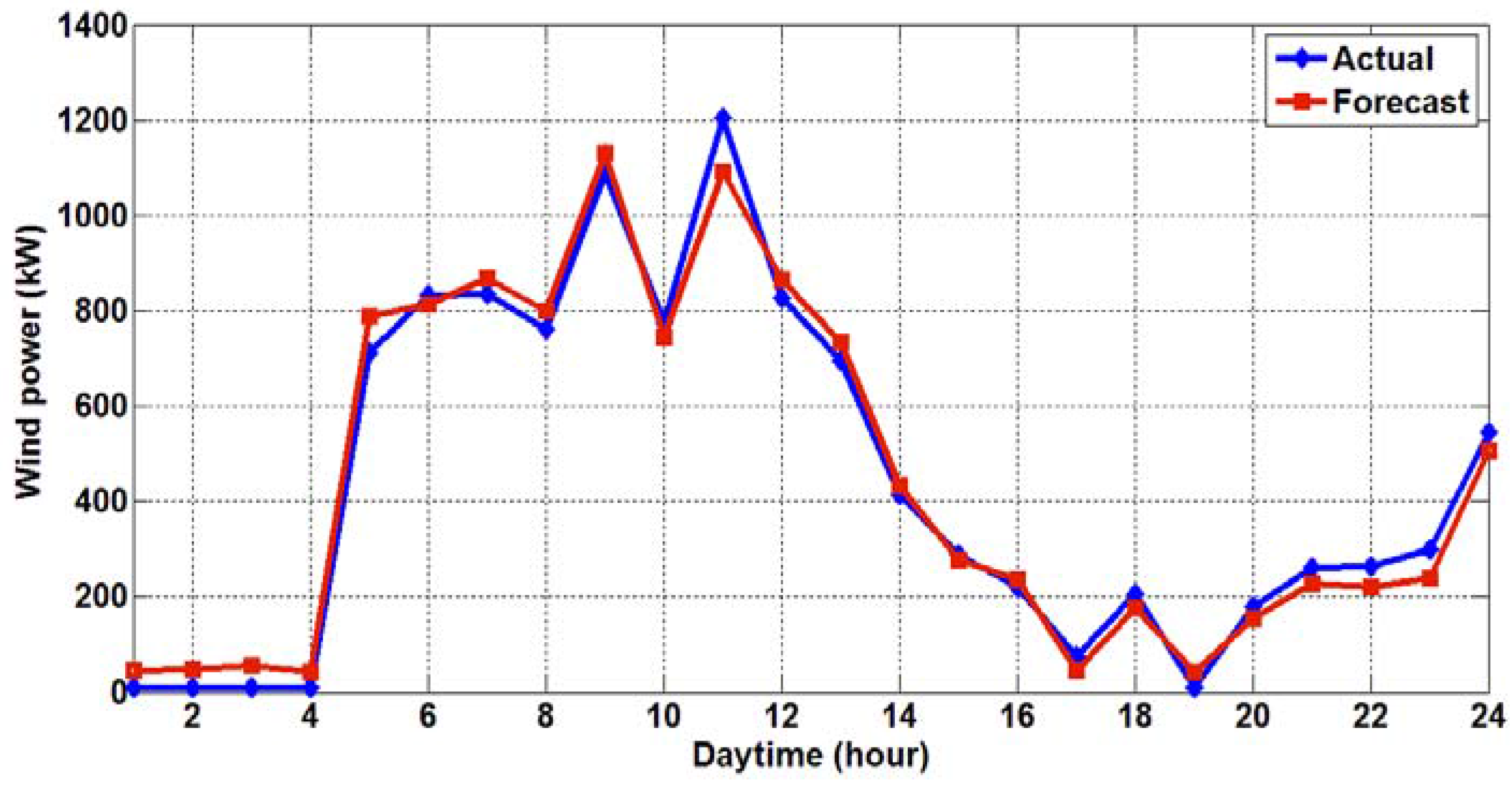
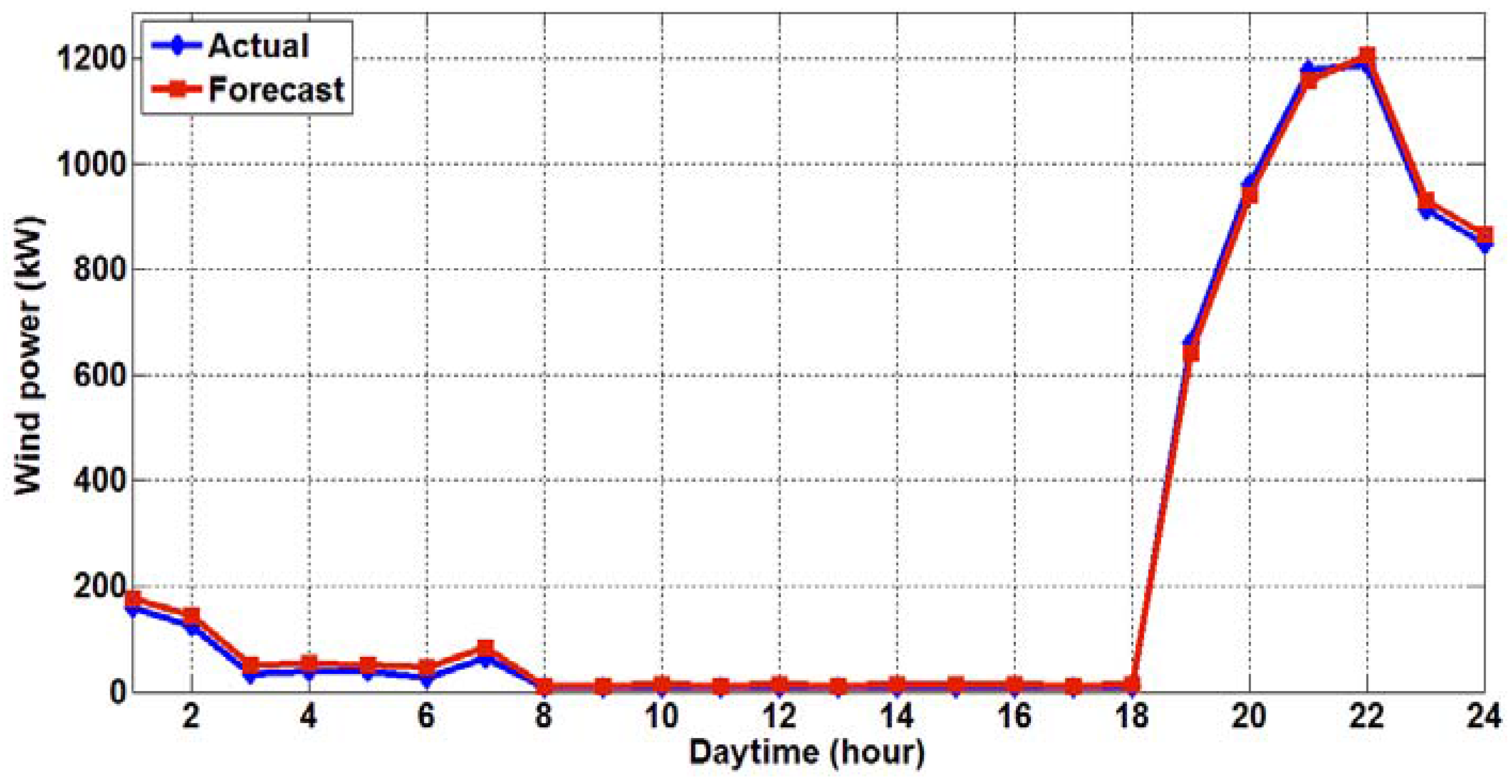
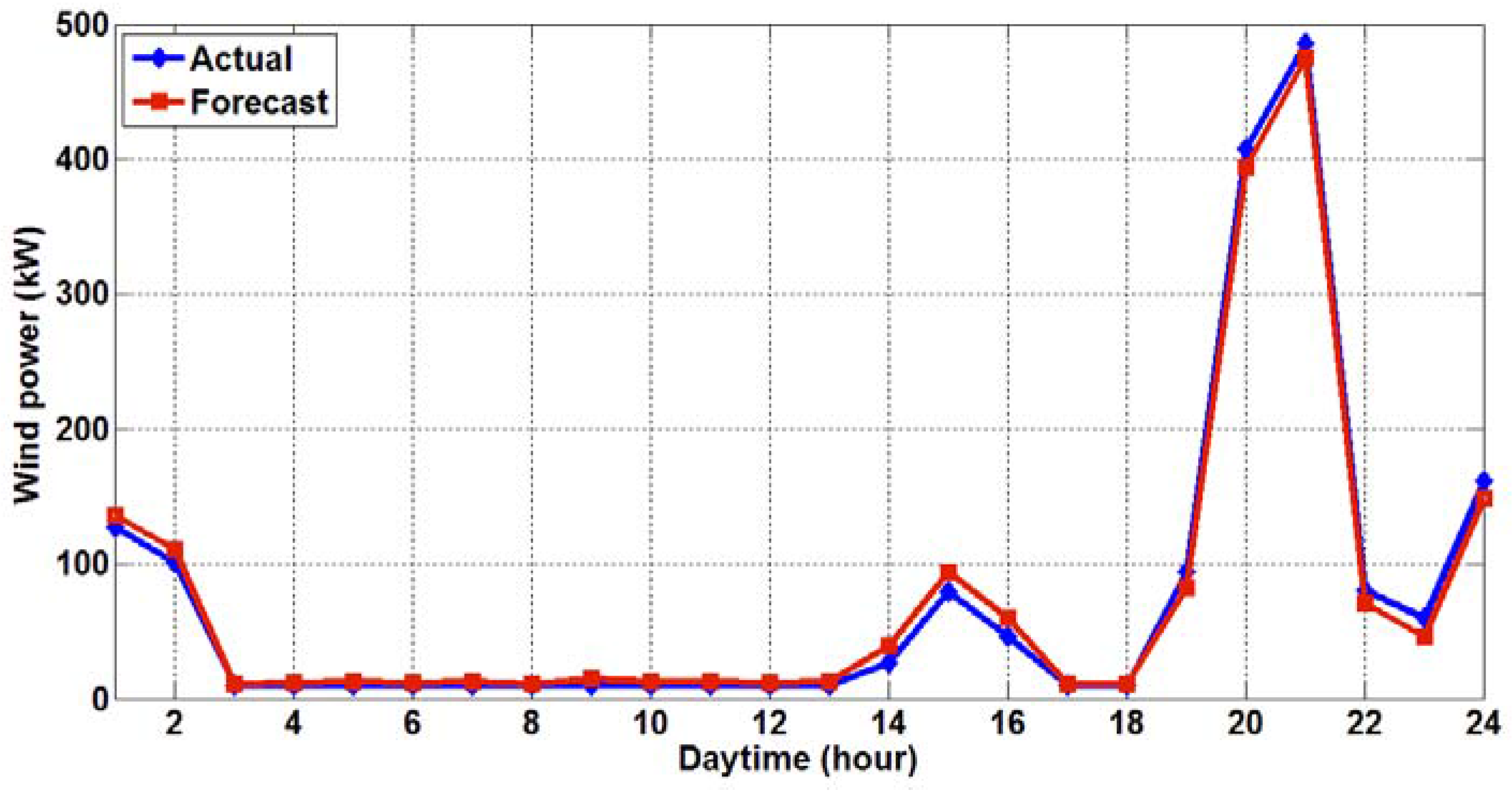
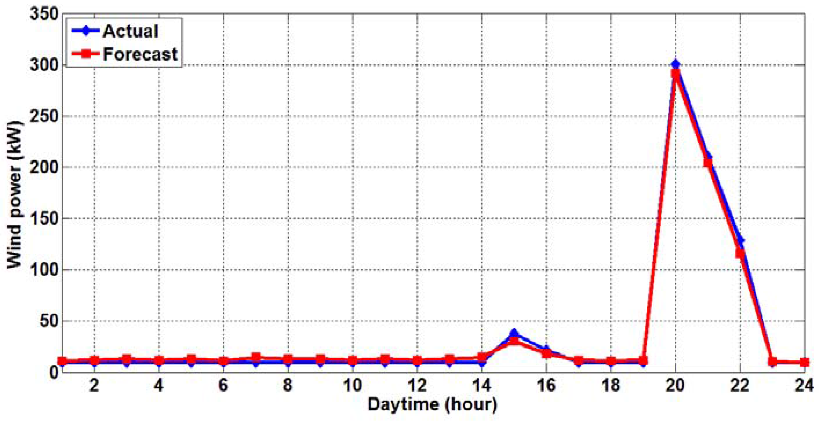
The forecasting information was presented for four days, representing the four seasons of the year: 21 July 2015, 15 October 2015, 4 January 2016, and 13 April 2016. For this reason, the days with the best wind power features were specifically and intentionally not selected. This provides an uneven accuracy allocation throughout the year that demonstrates the reality. The forecasting result was provided for each day with a time-step of one hour.

The forecasting results of the proposed two-stage hybrid HHT-GA-ANN model are shown in Figure 6, Figure 7, Figure 8 and Figure 9 for the winter, spring, summer, and fall days, respectively. Each figure illustrates the actual SCADA wind power record vs. the forecasted wind power result from the proposed model.

Table 3. Daily statistical error analysis of the forecast results by the proposed approach.

Day Type	MAPE (%)	$\sqrt{\mathrm{SSE}}$ (kW)	RMSE (kW)	SDE (kW)	Forecast Skill (%)
Winter	7.52	190.30	38.84	38.80	45.33
Spring	3.10	49.08	10.02	8.85	59.77
Summer	5.88	26.52	5.41	5.35	61.31
Fall	5.67	11.87	2.42	2.30	79.26
Average	5.54	69.45	14.17	13.82	61.42

presents the values of the metrics used to evaluate the accuracy of the two-stage hybrid HHT-GA-ANN model for forecasting wind power. The first column lists the day, the second column presents the daily MAPE, the third column presents the daily square root of the SSE, the fourth column presents the daily RMSE, the fifth column presents the daily SDE, and the sixth column presents the daily forecast skill.

Table 4. Comparative results of MAPE (%).

Forecast Model	Winter	Spring	Summer	Fall	Average
Persistence	13.52	7.33	16.10	27.58	16.13
BP-ANN	9.19	4.33	9.54	11.83	8.76
GA-ANN	8.68	4.22	9.01	9.40	7.83
Wavelet-GA-ANN	8.22	3.76	7.83	7.46	6.82
HHT-GA-ANN	7.52	3.10	5.88	5.67	5.54

gives a performance comparison between the proposed HHT-GA-ANN forecasting approach and four other approaches: Smart Persistence, BP-ANN, GA-ANN, and Wavelet-GA-ANN, with respect to the MAPE metric. The proposed approach resulted in better forecasting accuracy; the daily MAPE had an average value of 5.54%. The proposed approach’s average MAPE enhancement with respect to the other four approaches was 65.65%, 36.76%, 29.25% and 18.77%, respectively. The same training input-output datasets as those for the proposed approach were used for all of the other approaches. Moreover, all of the approaches were implemented with optimal parameter settings and configurations. The Daubechies-type discrete wavelet function of order 4 (Db4) was employed for the Wavelet-GA-ANN approach.

Table 5. Comparative NMAE (%) results.

Forecast Model	Winter	Spring	Summer	Fall	Average
Persistence	2.37	0.77	0.48	0.41	1.01
BP-ANN	1.61	0.46	0.29	0.17	0.64
GA-ANN	1.52	0.45	0.27	0.14	0.56
Wavelet-GA-ANN	1.44	0.40	0.23	0.11	0.55
HHT-GA-ANN	1.32	0.33	0.18	0.08	0.48

shows the forecast accuracy evaluation using the NMAE metric, considering the proposed HHT-GA-ANN approach and four other approaches (Smart Persistence, BP-ANN, GA-ANN, and Wavelet-GA-ANN).

With respect to the NMAE metric as given in Table 5, the proposed HHT-GA-ANN showed a mean error representing 0.48% of the installed wind power capacity for its 24-h-ahead forecasts across the entire prediction horizon.

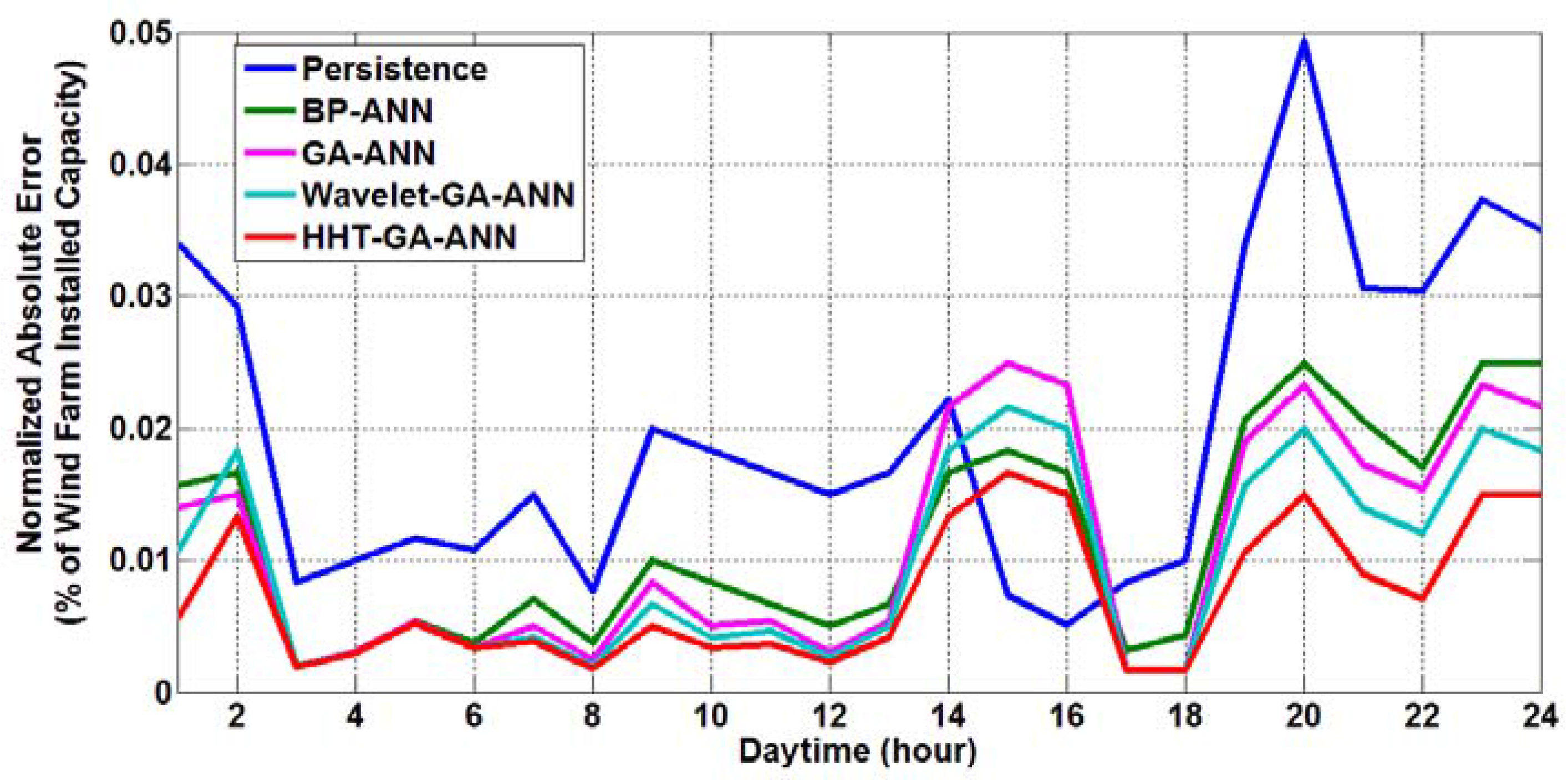
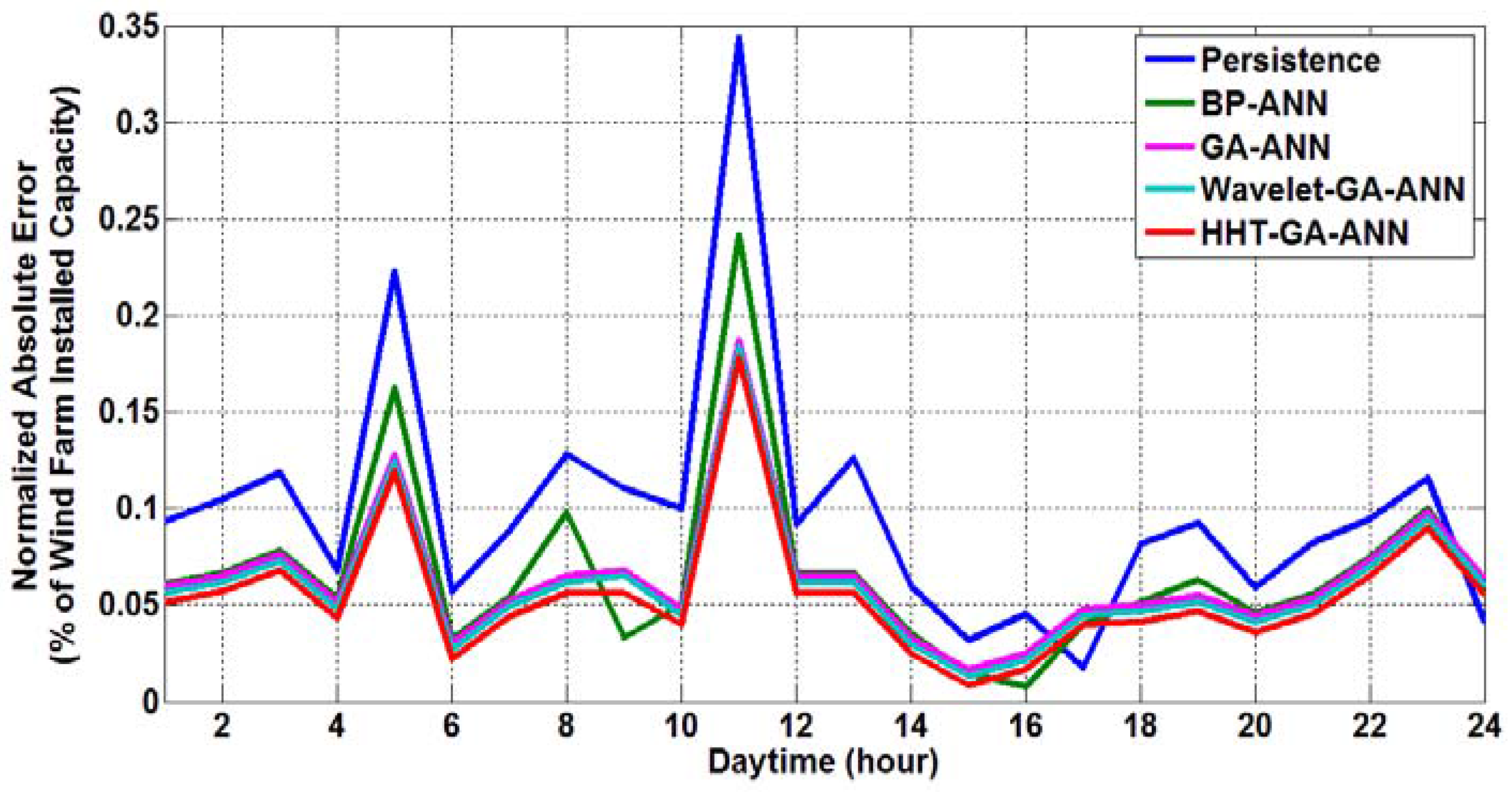
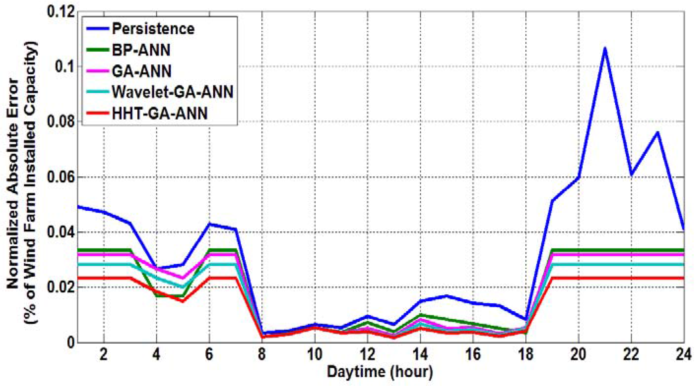
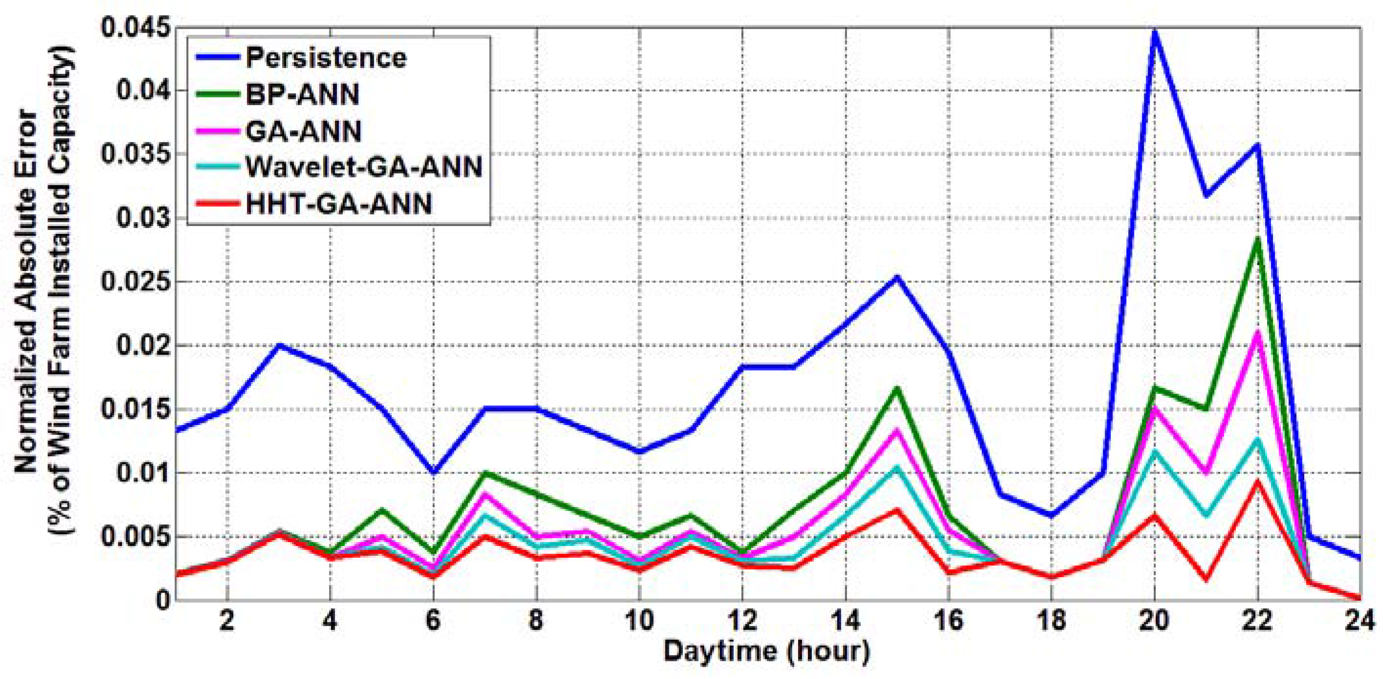
The absolute forecasting errors, on an hourly basis, with respect to the wind farm peak capacity (i.e., normalized by the peak wind farm capacity, NMAE), considering all of the approaches, are illustrated in Figure 10, Figure 11, Figure 12 and Figure 13, respectively, for the winter, spring, summer and fall days. As can be clearly seen from these figures, the proposed HHT-GA-ANN prediction approach gives the fewest normalized absolute errors when compared with the other four approaches.

In addition to the daily MAPE and NMAE metrics, consistency of prediction results is another important factor for comparing forecasting strategies.

Table 6. Daily prediction error variance.

Forecast Model	Winter	Spring	Summer	Fall	Average
Persistence	0.0079	0.0035	0.0089	0.0234	0.0109
BP-ANN	0.0042	0.0009	0.0038	0.0103	0.0048
GA-ANN	0.0022	0.0009	0.0046	0.0059	0.0034
Wavelet-GA-ANN	0.0022	0.0007	0.0034	0.0025	0.0022
HHT-GA-ANN	0.0022	0.0005	0.0017	0.0011	0.0014

gives a performance comparison between the proposed HHT-GA-ANN approach and the other four approaches (Smart Persistence, BP-ANN, GA-ANN, and Wavelet-GA-ANN), regarding the daily prediction error variance.

As given in Table 6, the mean prediction error variance was smaller for the proposed HHT-GA-ANN approach, demonstrating less uncertainty in the predictions. The proposed approach’s mean error variance enhancement in comparison to the other four approaches was 87.16%, 70.83%, 58.82% and 36.36%, respectively.

In addition to the aforementioned metrics, the forecast skill FS is a key performance indicator for different wind power forecasting models. It shows the quality of a forecast model by comparing its performance with respect to the smart persistence forecast.

Table 7. Comparative Forecast Skill (%) results.

Forecast Model	Winter	Spring	Summer	Fall	Average
Persistence	0.0	0.0	0.0	0.0	0.0
BP-ANN	25.56	33.61	28.96	40.60	32.18
GA-ANN	28.13	37.95	32.59	41.51	35.04
Wavelet-GA-ANN	32.59	40.91	37.71	42.48	38.42
HHT-GA-ANN	34.33	49.77	41.31	45.26	42.67

gives a performance comparison between the proposed HHT-GA-ANN approach and the other four approaches (Smart Persistence, BP-ANN, GA-ANN, and Wavelet-GA-ANN) in terms of the FS metric.

As indicated in Table 7, the proposed HHT-GA-ANN approach shows a much higher forecast skill for all days in all seasons of the year, reflecting its improved wind power forecasting quality.

For a more comprehensive comparison between the different wind power forecasting models used in this paper, representative statistical results for one year (from May 2015 to April 2016) are presented in

Table 8. Representative MAPE (%) results for a year (May 2015–April 2016).

Month	Persistence	BP-ANN	GA-ANN	Wavelet-GA-ANN	HHT-GA-ANN
May 2015	3.89	2.30	2.25	2.0	1.63
June 2015	43.95	26.04	24.60	21.37	16.05
July 2015	25.44	15.01	14.25	12.47	9.41
August 2015	16.74	9.88	9.37	8.20	6.19
September 2015	40.82	17.51	13.91	11.04	8.39
October 2015	44.13	18.98	15.00	11.91	8.83
November 2015	28.68	12.33	9.75	7.74	5.74
December 2015	16.49	11.21	10.59	10.03	9.17
January 2016	17.03	11.58	10.90	10.40	9.54
February 2016	22.31	15.17	14.28	13.61	12.50
March 2016	4.47	2.64	2.57	2.32	1.89
April 2016	5.13	3.03	2.97	2.67	2.15
Average	22.42	12.14	10.87	9.48	7.62

and

Table 9. Representative NMAE (%) results for a year (May 2015–April 2016).

Month	Persistence	BP-ANN	GA-ANN	Wavelet-GA-ANN	HHT-GA-ANN
May 2015	0.38	0.23	0.22	0.20	0.18
June 2015	0.76	0.46	0.43	0.36	0.28
July 2015	0.39	0.24	0.22	0.19	0.15
August 2015	0.46	0.28	0.26	0.22	0.17
September 2015	0.18	0.07	0.06	0.04	0.02
October 2015	0.20	0.08	0.07	0.05	0.03
November 2015	0.27	0.11	0.09	0.06	0.04
December 2015	1.73	1.17	1.11	1.05	0.96
January 2016	1.0	0.68	0.64	0.61	0.56
February 2016	2.58	1.75	1.65	1.57	1.44
March 2016	0.16	0.11	0.09	0.08	0.06
April 2016	0.26	0.16	0.15	0.13	0.11
Average	0.70	0.45	0.42	0.38	0.33

.

The proposed hybrid HHT-GA-ANN approach effectively outperforms all other approaches, as shown in Table 8 and Table 9.

Besides developing an effective wind power forecasting strategy, analysis of the impacts of input-data dependency (i.e., forecasting input-parameter selection) on the accuracy of the forecasting model is critical in implementing a robust wind power prediction model.

In this study, the impact of the forecasting input dataset dependency on the prediction accuracy of the proposed approach is investigated by dividing the forecasting input dataset into five subsets; where dataset #1 contains only wind speed, dataset #2 consists of wind speed and wind direction, dataset #3 consists of wind speed, wind direction and air temperature, dataset #4 consists of wind speed, wind direction, air temperature and air pressure, and dataset #5 consists of wind speed, wind direction, air temperature, air pressure and air humidity.

Table 10. Comparative MAPE (%) results of different input datasets.

Data Subset	Winter	Spring	Summer	Fall	Average
Subsets #1	9.78	4.66	7.44	7.23	7.28
Subsets #2	8.17	4.15	6.7	6.8	6.45
Subsets #3	7.89	3.51	6.4	6.4	6.05
Subsets #4	7.6	3.47	6.25	6.2	5.88
Subsets #5	7.52	3.10	5.88	5.67	5.54

shows a performance comparison between all five datasets with respect to the MAPE metric. The proposed prediction approach with input dataset #5 results in better prediction accuracy; the MAPE has a mean value of 5.54%. The proposed approach’s mean MAPE enhancement using input dataset #5 in comparison to the four other datasets is 23.90%, 14.11%, 8.43% and 5.78%, respectively.

The proposed two-stage hybrid HHT-GA-ANN approach results in better performance with respect to forecast accuracy and skill, outperforming the other four approaches. Moreover, the mean computational time was about 30 s, using the MATLAB simulation environment on a personal computer with Intel core i5-5200 CPU, 2.20 GHz processor and 4 GB RAM. Hence, the proposed approach is both novel and effective for day-ahead or short-term wind power prediction.

7. Conclusions

In this paper, a novel two-stage hybrid approach was proposed for day-ahead wind power prediction, considering both statistical (wind power SCADA records) and physical (NWP meteorological variables) data inputs. The proposed approach was based on a combination of HHT, GA and ANN. The basic forecasting tool employed was the MLFF ANN. The HHT was utilized to decompose the NWP meteorological data series and SCADA wind speed and power data series into a set of improved-characteristic subseries. The GA was used to optimize the ANN weight parameters to achieve higher forecasting accuracy and improved performance. The proposed approach has two hybrid HHT-GA-ANN stages. In the initial stage, HHT-GA-ANN is implemented to forecast wind speed at the exact wind turbine hub height on the wind farm installation site. In this stage, historical NWP meteorological variables are used as inputs, and historical actual wind speed SCADA measurement records are used as the target output to train the ANN. In the second stage, HHT-GA-NN is modeled to map the wind speed versus power characteristics solely based on actual wind farm SCADA historical records. Then, the predicted wind speed from the HHT-GA-ANN model in the initial stage is fed to the developed (trained) HHT-GA-ANN model in the second stage, in order to forecast the future output power of the wind farm. One-year historical NWP meteorological data (wind speed, wind direction, air pressure, air temperature and humidity) and SCADA wind speed and power data were used to construct the forecasting model of the proposed approach. The model has the capacity to be retrained periodically when new input data is available. The implementation of the proposed approach for day-ahead wind power prediction is both novel and effective. The daily average values of MAPE, NMAE, and FS were 5.54%, 0.48% and 42.67%, respectively, outperforming four other wind power forecast models, while the mean computation time was less than 30 s. Thus, the demonstrated numerical results verify the effectiveness of the proposed approach for a day-ahead wind power forecast.