H-Shaped Multiple Linear Motor Drive Platform Control System Design Based on an Inverse System Method


1
Department of Mechanical Engineering, Korea Advanced Institute of Science and Technology, Daejeon 34141, South Korea
2
School of Electrical Engineering and Automation, Harbin Institute of Technology, Harbin 150001, China
3
Faculty of Technology Policy and Management, Delft University of Technology, 2628 BX Delft, The Netherlands
*
Author to whom correspondence should be addressed.
Energies 2017, 10(12), 1990; https://doi.org/10.3390/en10121990
Submission received: 11 October 2017
/
Revised: 13 November 2017
/
Accepted: 21 November 2017
/
Published: 1 December 2017
(This article belongs to the Section I: Energy Fundamentals and Conversion)
Abstract
:Due to its simple mechanical structure and high motion stability, the H-shaped platform has been increasingly widely used in precision measuring, numerical control machining and semiconductor packaging equipment, etc. The H-shaped platform is normally driven by multiple (three) permanent magnet synchronous linear motors. The main challenges for H-shaped platform-control include synchronous control between the two linear motors in the Y direction as well as total positioning error of the platform mover, a combination of position deviation in X and Y directions. To deal with the above challenges, this paper proposes a control strategy based on the inverse system method through state feedback and dynamic decoupling of the thrust force. First, mechanical dynamics equations have been deduced through the analysis of system coupling based on the platform structure. Second, the mathematical model of the linear motors and the relevant coordinate transformation between dq-axis currents and ABC-phase currents are analyzed. Third, after the main concept of inverse system method being explained, the inverse system model of the platform control system has been designed after defining relevant system variables. Inverse system model compensates the original nonlinear coupled system into pseudo-linear decoupled linear system, for which typical linear control methods, like PID, can be adopted to control the system. The simulation model of the control system is built in MATLAB/Simulink and the simulation result shows that the designed control system has both small synchronous deviation and small total trajectory tracking error. Furthermore, the control program has been run on NI controller for both fixed-loop-time and free-loop-time modes, and the test result shows that the average loop computation time needed is rather small, which makes it suitable for real industrial applications. Overall, it proves that the proposed new control strategy can be used in industrial applications that have high-precision and high real-time performance requirements.
1. Introduction
In the manufacturing industry, some complex curve or special trajectory is needed to produce high-precision industrial products. For instance, planar motion is needed in pick-and-place machines, semiconductor lithography, CNC machine tools and transport devices [1,2]. A traditional platform has normally been driven by a rotatory motor with ball screw, which has numerous disadvantages, such as mechanical drive links, large response lag and nonlinear friction. Linear motor direct drive can avoid unnecessary mechanical links, which thus can improve the positioning accuracy of the platform. The combination of multiple linear motors has been adopted to achieve movement in multiple degrees of freedom [3]. The H-shaped platform is a Cartesian movement platform with a special structure consisting of three linear motors. It features many advantages, such as simple structure, high precision and high stability. Compared with other linear motors, permanent magnet synchronous linear motor has high control precision and fast dynamic response, thus it has been widely used in H-shaped platform.
On the H-type platform of multiple permanent magnet synchronous linear motors drive, there is inevitable deviation between the two linear motors in the Y direction. If the displacement deviation between them exceeds some limit, the motion accuracy cannot be guaranteed. Moreover, the platform structure and the drive components might be destroyed. Therefore, decreasing the synchronization deviation to be within an acceptable range is one of the major issues in the control of multiple linear motors [4,5]. Over the past decade, the cross-coupled control technology has been majorly used in machine tools and multiple axes motion applications for reducing contour tracking errors [6,7,8,9]. In the cross-coupled control, the comparison of two motors’ position or speed signal is calculated and the deviation is then used as the extra feedback signal. The extra feedback is often used as the tracking signal based on which the control system can adjust accordingly to the load change of any motor, and thus it can realize high synchronous control precision. Recently, cross-coupled technology has been incorporated with some well-known adaptive control approaches to solve the synchronous control problem and to improve the control performance [10,11,12].
Relevant research has also been done for the application of H-shaped platform driven by multiple linear motors. An interval type-2 fuzzy neural network control method has been presented for H-type gantry stage driven by dual linear motors in [13]. The proposed method has set the position error between the two side motors as input, and the powerful self -learning ability of neural network is used to guarantee the synchronous error converges to zero to achieve synchronous control. A cross-coupled intelligent complementary sliding mode control system has been proposed for the synchronous control of a dual linear motor servo system installed in a gantry position stage in [14]. For the problem that a dual linear motor servo system on the X-axis of gantry moving machining centers is not synchronized during the driven process, paper [15] has proposed an improved variable structure control and decoupling control approach, through which not only the synchronization accuracy is upgraded but also the chattering problem of the ideal sliding mode is avoided. The trajectory control of the H-shaped platform in this paper is realized by three linear motors. The above control strategies focus on the synchronous control of two linear motors in the Y direction, which is independent from the control of the third perpendicular motor X. In the above independent control strategies, the platform total positioning error is the combined result of the positioning errors in X and Y directions. With the goal to decrease the total positioning error and improve the control precision, this paper proposes to integrate the three motors into one whole control system instead of performing the control in X and Y directions independently.
Overall, the H-shaped platform driven by multiple (three) linear motors is a very complex nonlinear control system. Moreover, the variables are cross-coupled with each other, and thus the dynamic decoupling control of their speeds is necessary. Without being relied on the nonlinear system solution and stability analysis, the inverse system method only deals with the feedback transformation, and thus it can be seen as a more general method. Feedback linearization is used in the inverse system method to realize the linear decoupling of a multi-variable, nonlinear and coupled system. This method has been widely used in control systems because it is highly intuitive and simple, and has high decoupling control performance. Paper [16] has presented a novel control scheme combining the inverse system method and the internal model control, which enhances the control accuracy and dynamic performance of a bearing-less permanent magnet synchronous motor. To radically eliminate the influence of gyroscopic effects on system stability and to improve the performances of high-precision, fast-response for the high-speed magnetically suspended rotor system in a control moment gyro, paper [17] has proposed a control strategy that combines inverse system method and internal model control. Paper [18] adopts feedback linearization control of three-phase inverter based on inverse system, in which to guarantee symmetric output voltage with asymmetric load for three-phase inverter, a feedback linearization based on inverse system for three-phase inverter has been proposed, which can improve system adaptability and stability under complex load conditions and disturbances.
In order to decrease the synchronous deviation and total positioning error, this paper proposes a new control strategy based on the inverse system method to realize the decoupling control of an H-shaped platform driven by multiple linear motors. Not only can the proposed control method deal with the coupling issue of multiple motors and decrease the total positioning error, but it can also meet the real-time computation requirements in practical industrial applications because classical simple PID (proportional-integral-derivative) control strategy can be used in the pseudo-linear decoupled system.
2. An H-Type Platform Driven by Multiple Permanent Magnet Synchronous Linear Motors
2.1. Platform Structure
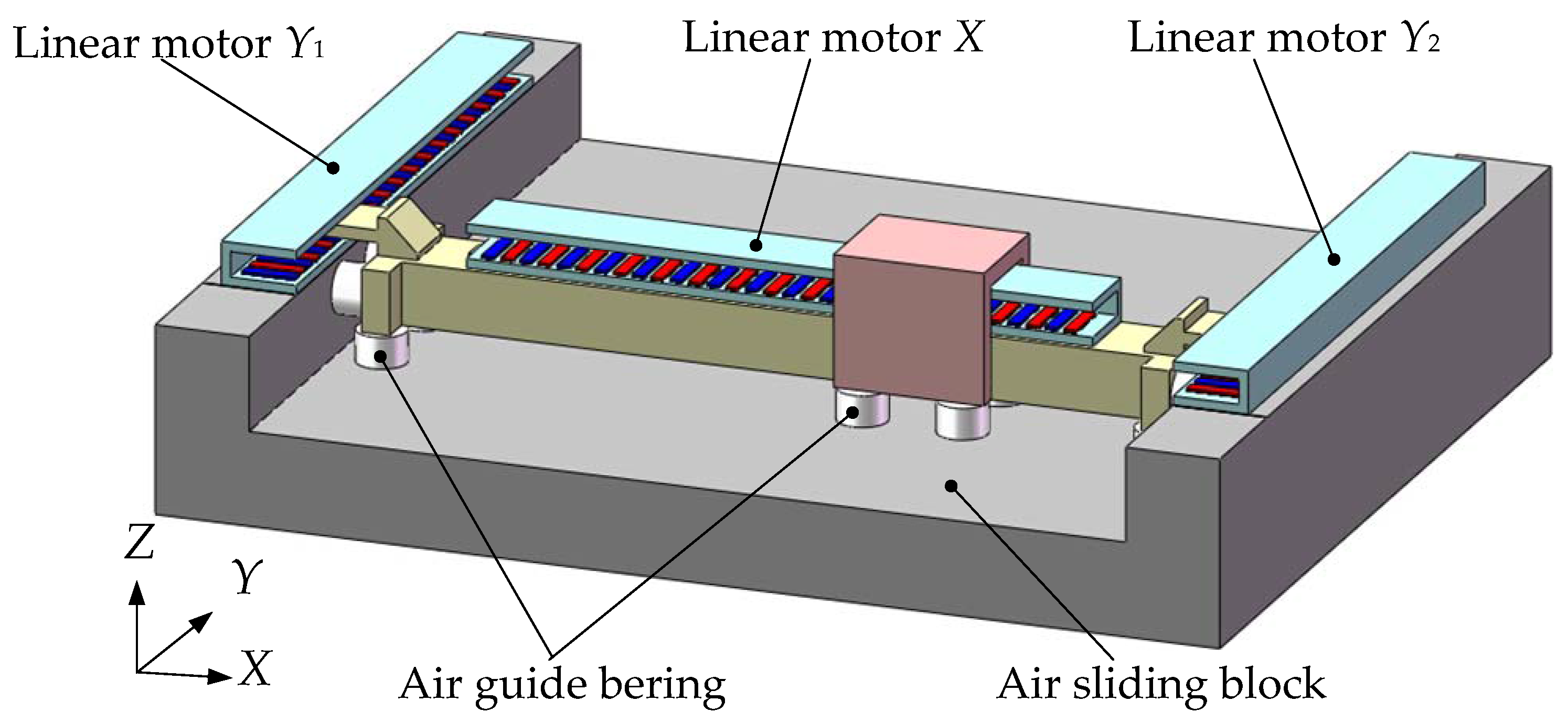
The H-type platform driven by multiple permanent magnet synchronous linear motors is shown in Figure 1. This high-precision platform adopts gas guide bearing. The crossbeam is made of light, high-stiffness, low-density alloy materials and the two ends of it are connected to the movers of the two linear motors in Y direction (motor Y1 and Y2), which realize the bilateral synchronous drive in Y direction. The stator of the linear motor in X direction is fixed on the crossbeam and the mover of it is connected to the air sliding block, which realizes the motion in the X direction. Both the crossbeam and the slide block are sustained and guided by the air bearing. The planar movement in the XY plane can be realized through the control of the three linear motors. In practical control, there will also be rotation around the axis of Z due to the deviation between the two linear motors in Y direction. In practical control, the goal is to make the deviation approach zero. It can be seen from the above analysis that there is mechanical coupling between the three linear motors.
Even though the two linear motors (Motor Y1 and Y2) moving in the Y direction and their servo systems can be designed to have the same parameters, in practical control process the synchronization of the two motors cannot be guaranteed due to the position change of the motor moving in the Y direction. The position of the linear motor moving in the X direction also changes in the working process, and thus the distance between it and the two linear motors moving in the Y direction also changes accordingly, which influences the force allocated to each motor. Moreover, the machining error is inevitable in the process of manufacturing and installation. In addition, there is always uncertain disturbance during the operation. Therefore, there is high requirement for the control system to make sure the synchronous deviation is within a certain small range.
2.2. Mechanical Analysis
Figure 2 shows a simplified diagram of force imposed on the crossbeam when there is a small rotation angle δ. It should be noted that the rotation angle δ in Figure 2 is presented to be unreasonably large for the purpose of simple understanding. In practice, the angle δ needs to be controlled within an extremely small range (less than 0.1°). The two linear motors, motor Y1 and motor Y2, can produce horizontal forces fY1, fY2. Not only can the two forces contribute to the motion in X and Y direction, but also the difference between them can contribute to the rotation movement around Z-axis. With the forces generated by the three linear motors projected on X-axis and Y-axis, we can get the following equations:
Based on Newton’s motion law, we can further get the following equations:
where m is the mass, J is rotary inertia, and l represents the distance between fY1 and fY2. According to the control requirement, δ is constrained to be less than 0.1°, thus cosδ approaches 1 and sinδ approaches 0. The above equations can be then further simplified as:
3. Pre-Analysis for Permanent Magnet Synchronous Linear Motor Control System
3.1. ABC Coordinate System to d-q Coordinate System
The three-phase AC motor can be seen as a DC motor through coordinate transformation. The three-phase currents can be transformed into force current iq (proportional to the electromagnetic force) and magnetic field excitation current id. The transformation can be divided into two steps.
First, ABC coordinate system is transformed to the static α-β coordinate system:
Second, the static coordinate system is then further transformed to the dynamic d-q coordinate system:
Based on the above two transformations, the inverse transformation is shown as:
Through Equation (6), it can be known that the needed three-phase currents can be calculated from the desired id and iq.
3.2. Mathematical Model
In dq-axis reference frame, the voltage and flux link relations of the permanent magnet synchronous linear motor are shown in the following equations:
where ud, uq, id, iq, Ψd, Ψq, Ld, Lq are dq-axis voltage, current, flux linkage, and inductance respectively. Rs is the primary resistance; Ψf is the permanent flux linkage; v is the mover’s velocity; P is the number of pole pairs [19,20,21].
The mathematical expression relating the thrust force to the current for a salient permanent magnet synchronous linear motor is given as:
where FT is the electromagnetic thrust force; and τ is the pole pitch.
For a surface mounted synchronous motor, Ld = Lq and thus the equation above can be simplified into equation:
It can be known from Equation (13) that the horizontal electromagnetic force can be controlled by iq, current in q-axis, with other parameters fixed.
3.3. PID Controller
PID controller (see Figure 3) is one of the simplest and most robust control methods; thus, it has been widely used in numerous industrial applications. Due to its simple algorithm, PID controller can be very time-efficient in terms numerical computation and thus it has been adopted in this paper. PID controller is a classical controller whose time domain expression and transfer function are:
where Kp, Ki, Kd are the proportional gain, integral gain and differential gain, respectively. The system input can be seen as the sum of the proportional component, integral component and differential component. The proportional component is essential for decreasing the general control error; the integral component makes the stable state error approach zero and the differential component can improve the dynamic trajectory following performance especially when there is a sudden (high-frequency) change for the system output.
As a classical linear control method, PID can be used in this control system because the inverse system model compensates the original nonlinear coupled system into a pseudo-linear decoupled linear system. The inverse system method will be introduced in the next part of the paper.
4. Inverse System Model and Control System Design
The basic idea of inverse system model can be described as follows: For a given system, α-th order integration inverse system model can be built through the feedback method based on the original system model. The inverse system model compensates the original system into a new linear and decoupled normalized system that is often called a pseudo-linear system. Then, all the linear control theories can be used to integrate the above pseudo-linear system. It is called pseudo-linear because the compensated system has a linear transfer function but the relationship inside the internal variables might still be nonlinear.
4.1. Inverse System Decoupling
4.1.1. Inverse System Theory
For a given nonlinear system Σ, multivariable state equation is shown as:
where u(t) ∈ Rm is the input vector, y(t) ∈ Rr is the output vector, x(t) ∈ Rn is the state variable, and the initial condition is x(t0 ) = x0, r ≤ m.
For the output function y = h(x, u), we can deduce the αi-th order derivative of yi to time variable t, which is shown as:
where the value of αi (1 ≤ i ≤ r) is defined as:
In the above equation, for 1 ≤ i ≤ r, we have αi < ∞, otherwise it is not derivable.
Based on Equation (17) the inverse system can be derived as:
where
Then a new system equation can be derived as:
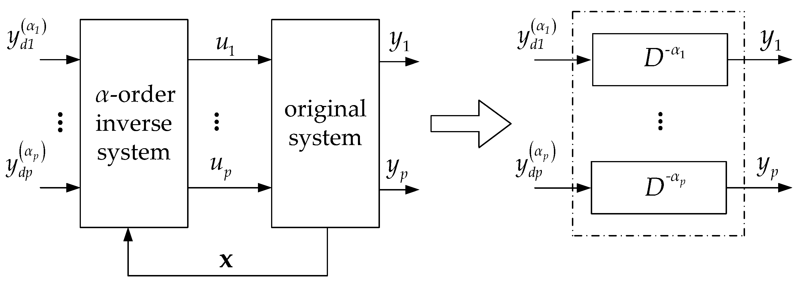
The system can be seen as the α-th order inverse system of the original system Σ. It can be seen that the pseudo-linear system has a linear transfer function between the input and the output which are decoupled. As shown in Figure 4, the output of the α-th order integration inverse system is connected to the input of the original system; yd(t) is the expected (reference) output of the original system and, y(t) is the real output of the original system. The state variables of the original system are used in the α-th order integration inverse system through feedback. The expected output value can then be the input of the system controller.
4.1.2. Inverse System Condition
Obviously, not every system has its inverse system because some conditions need to be satisfied. It can be known form Equation (16) that the nonlinear system has relative order {α1, α2, ···, αr} at (x0, u0). Two basic conditions need to be satisfied as follows.
- At (x0, u0), the following equation is satisfied:where is the k-th order Lie derivative.
- The r × m order matrix shown as follows is nonsingular, which indicates the rank of the matrix .
A given system is invertible in a range around (x0, u0) when the above {α1, α2, ···, αr} exists and they meet the requirements of the following equation where n is the number of system state variables:
4.2. H-Shaped Platform State Equation
The basic idea of controller design can be explained as follows. Based on the mathematical model of the dual linear motor control system, the α-th order integral inverse system can be derived from the previous system via feedback linearization. The inverse system turns the previous nonlinear and coupling system into a pseudo-linear and decoupling system, which can be analyzed by the traditional linear control theory.
The state variables of the system are set to be
The output variables of the system are set to be
The input variables are set to be
Based on Equations (3) and (13), we can get
where
Combining Equation (28) with the state variables, we can get
4.3. Decoupling Design
It can be seen from Equations (28)–(30) that the H-shaped platform is a nonlinear coupled system with three inputs and three outputs. It remains to be checked whether the system is invertible. We can first get the following equation through calculating the derivative of y = [y1, y2, y3]T and it contains u = [u1, u2, u3]T.
It can be seen from the above equation that
The rank of is equal to 3 and thus it is non-singular. The relative derivative orders α = {α1, α2, α3} = {2, 2, 2} = 6, which is equal to the number of state variables. Thus, the system is invertible. Suppose:
We can get the state feedback equation
Based on the state feedback described as in Equation (31) it can be known that the new system is a linear system without coupling, denoted as follows:
4.4. Control System Structure
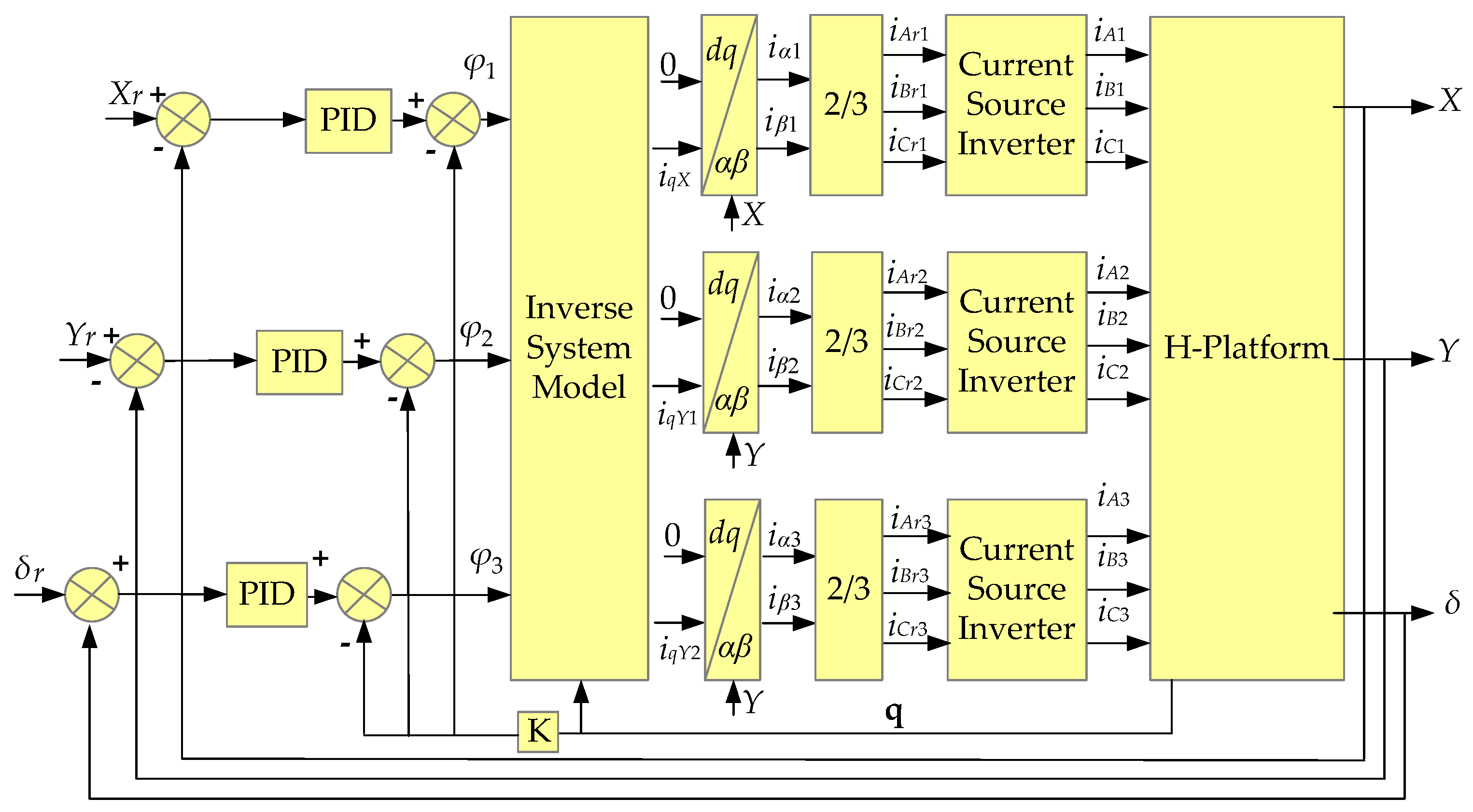
Based on the above analysis, the control system of the H-shaped platform is as shown in Figure 5. The control system includes PID controller, inverse system model, control current coordinate transformation and the H-shaped platform itself.
As Figure 5 shows, the control system has three reference signals, which are the given position Xr, position Yr and rotation angle around Z-axis δr. The feedback actual values are compared with the given values and the difference between them will be used for PID position regulation. The regulation results are used to compare with the state feedback values, and the difference between them is further used as the input of the inverse system model. Vector control with id = 0 is chosen as the control strategy because the magnetic field is kept constant and only iq is used to control the thrust force of the linear motor. The needed force-generating current iq can then be calculated through the inverse model. After the coordinate transformation, the dq-axis current can be transformed into the three-phase currents, which will be fed to the linear motor after the power amplifier.
5. Simulation and Analysis
The proposed control strategy has been validated in Matlab/Simulink. First, the synchronous deviation between the two linear motors Y1 and Y2 is analyzed. Second, the proposed control method is compared with the traditional method in terms of its performance for the mover trajectory under disturbance. Lastly, the program has been implemented on NI controller which is a typical industrial controller. The motor in this paper is a maglev permanent magnet linear synchronous motor, whose basic electromagnetic model parameters are show in Table 1.
5.1. Synchronous Deviation Analysis
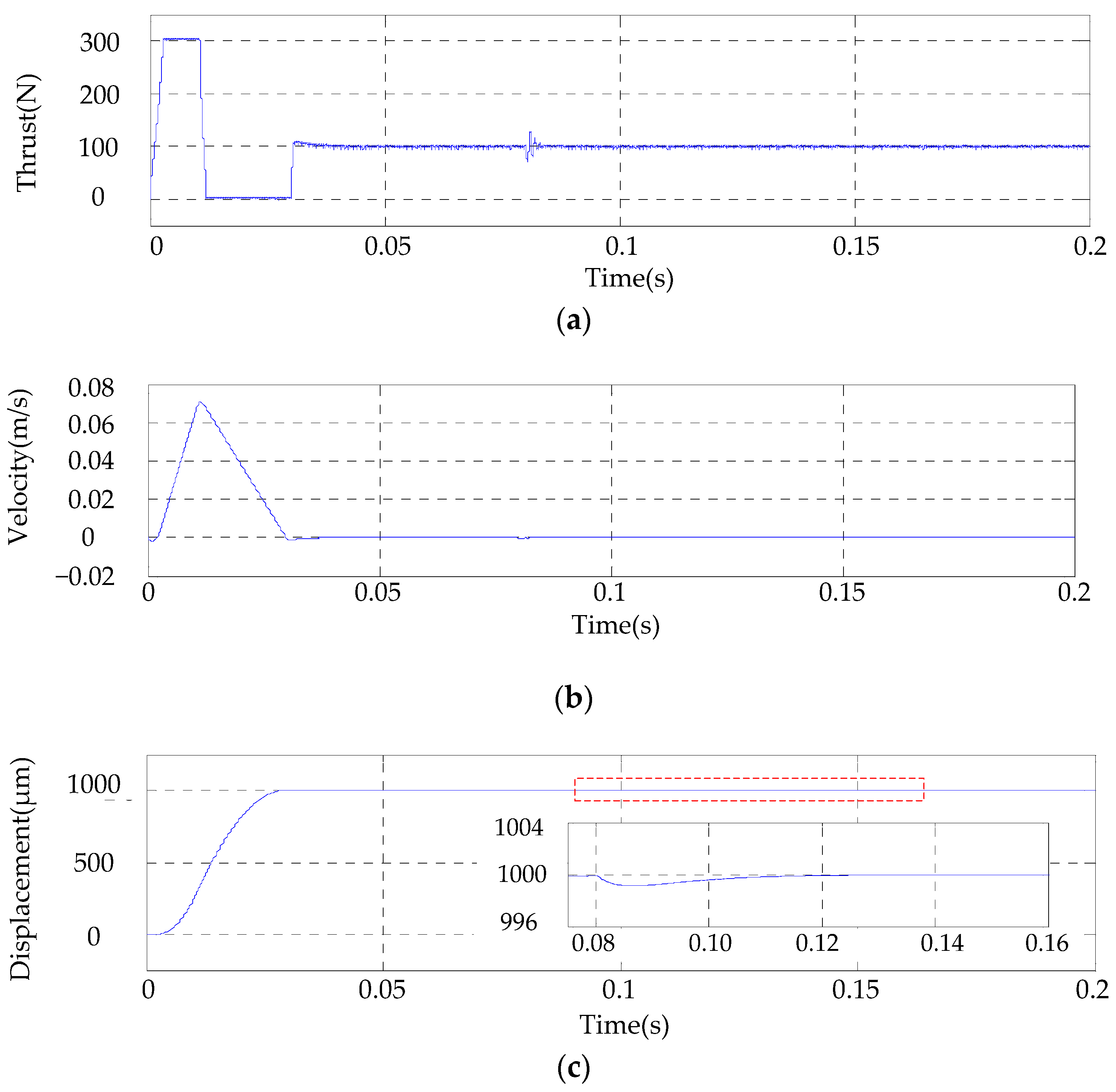
In the control process, when disturbance is imposed on one motor (either Y1 or Y2) causing the synchronous deviation, the controller will control both Y1 and Y2 to decrease the deviation between them. The simulation time is set to be 0.2 s. The given reference position for the two linear motors Y1 and Y2 is 1000 μm. The load force on Y1 and Y2 are 100 N, and at 0.08 s the load force imposed on Y1 is increased to 150 N. The electromagnetic force on Y1 and displacement of Y1 is shown in Figure 6. The result for Y2 is shown in Figure 7.
Figure 6a shows that the load disturbance is imposed at 0.08 s, causing a displacement change of up to about 1 μm for linear motor Y1 as shown in Figure 6c. To keep synchronous with Y1, the electromagnetic force and displacement of Y2 also changes. The position control of the motor consists of three major phases: acceleration phase, deceleration phase and positioning/stable phase. It can be seen from Figure 6a and Figure 7a that the thrust torque at the start phase approaches 300 N (the maximum motor thrust force), which corresponds to the velocity increase phase in Figure 6b and Figure 7b. When the motor approaches the reference position, it enters the deceleration phase, which occurs at about 0.01 s after the start. Finally, the motor arrives at the given position and its speed also decreases to zero, which indicates the motor is in the positioning or stable phase. In the positioning phase, the position of the motor keeps constant and the thrust force is equal to the load force.
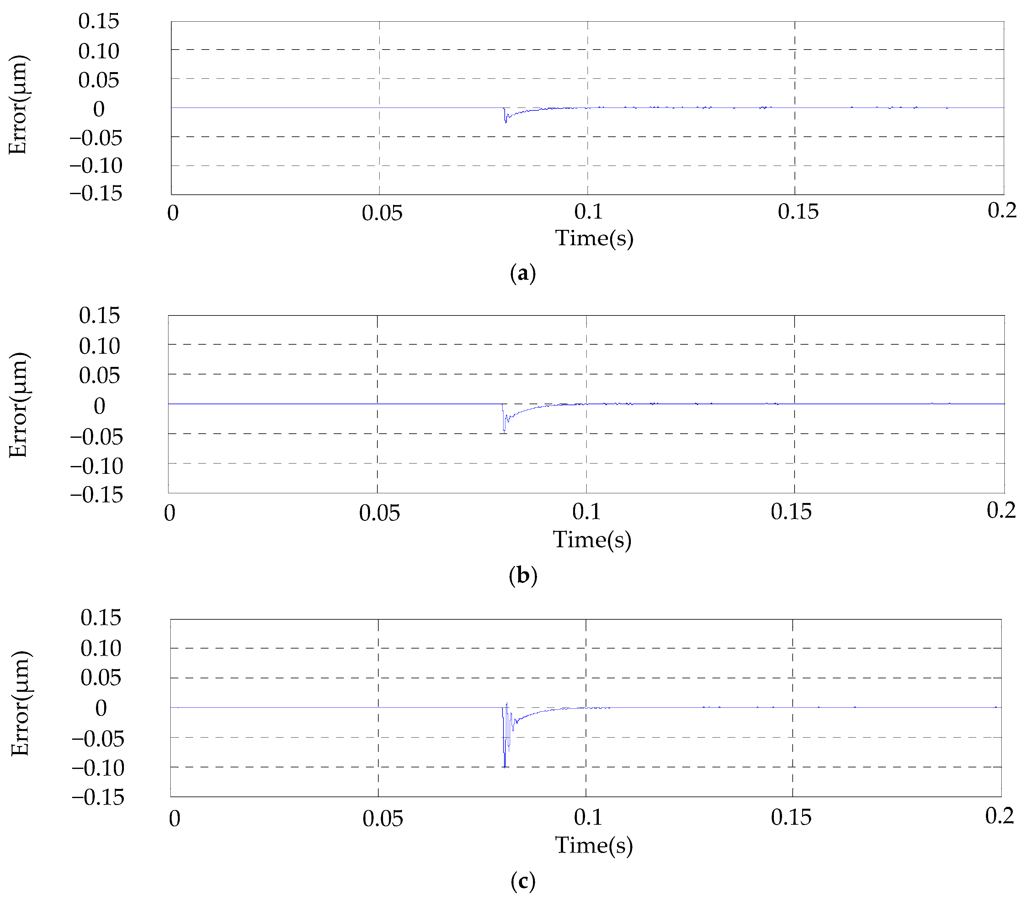
Figure 8 shows the synchronous deviation between Y1 and Y2 when it is under the disturbance force of 20 N, 35 N and 50 N. It shows the maximal synchronous deviation is 0.025 μm, 0.05 μm, when the load force is 20 N and 35 N respectively. The recovery time under different disturbances is 0.02 s, while the synchronous deviation increases nonlinearly with the increase of disturbance. For the disturbance of 50 N (half the rated load force), the maximal synchronous deviation between them is 0.1 μm with a recovery time of 0.02 s. It proves that the proposed control strategy can meet the high-precision and fast-response dynamic requirements in planar positioning applications.
5.2. H-Platform Trajectory Analysis
The simulation period for the trajectory analysis is set to be 0.2 s. The trajectory of the H-shaped platform is the combined result of the movement in the X and Y directions. More specifically, the H-shaped platform trajectory can be seen as the movement of the center of mass for the linear motor X. The given reference position in the X and Y directions are both 10 μm. Load force disturbance lasting a short period is very common in the practical control process. The control system should show strong robustness under such disturbance force at random direction. At 0.08 s the load disturbance forces of 100 N (half the sum of the rated forces for the two linear motors Y1 and Y2) in the Y direction and 50 N (half the rated force for linear motor X) in the X direction, both of them lasting for 0.005 s, are imposed on the platform mover to simulate such random disturbance forces. Figure 9 shows the simulation result for both the proposed new control method and traditional PID method.
Figure 9a shows the trajectory of the H-shaped platform adopting the proposed inverse system-based PID control strategy, while Figure 9b shows that for the H-shaped platform adopting traditional independent PID control strategy. The simulation result shows that the trajectory in Figure 9a has a significantly smaller deviation from the given reference position than that in Figure 9b. Traditional PI strategy controls the X and Y direction movement independently. However, the proposed new control strategy integrates them into one control model. The smaller deviation from the given reference position in Figure 9a shows that the total trajectory error, which is the combination of that in X and Y direction, in the proposed new control model is smaller. In practical manufacturing process, it means the proposed control strategy can guarantee the platform mover moves along the given reference trajectory with only a tiny deviation even under the sudden short-period disturbance forces. Thus, compared with the traditional independent PID, the proposed control strategy has better dynamic and robust performance.
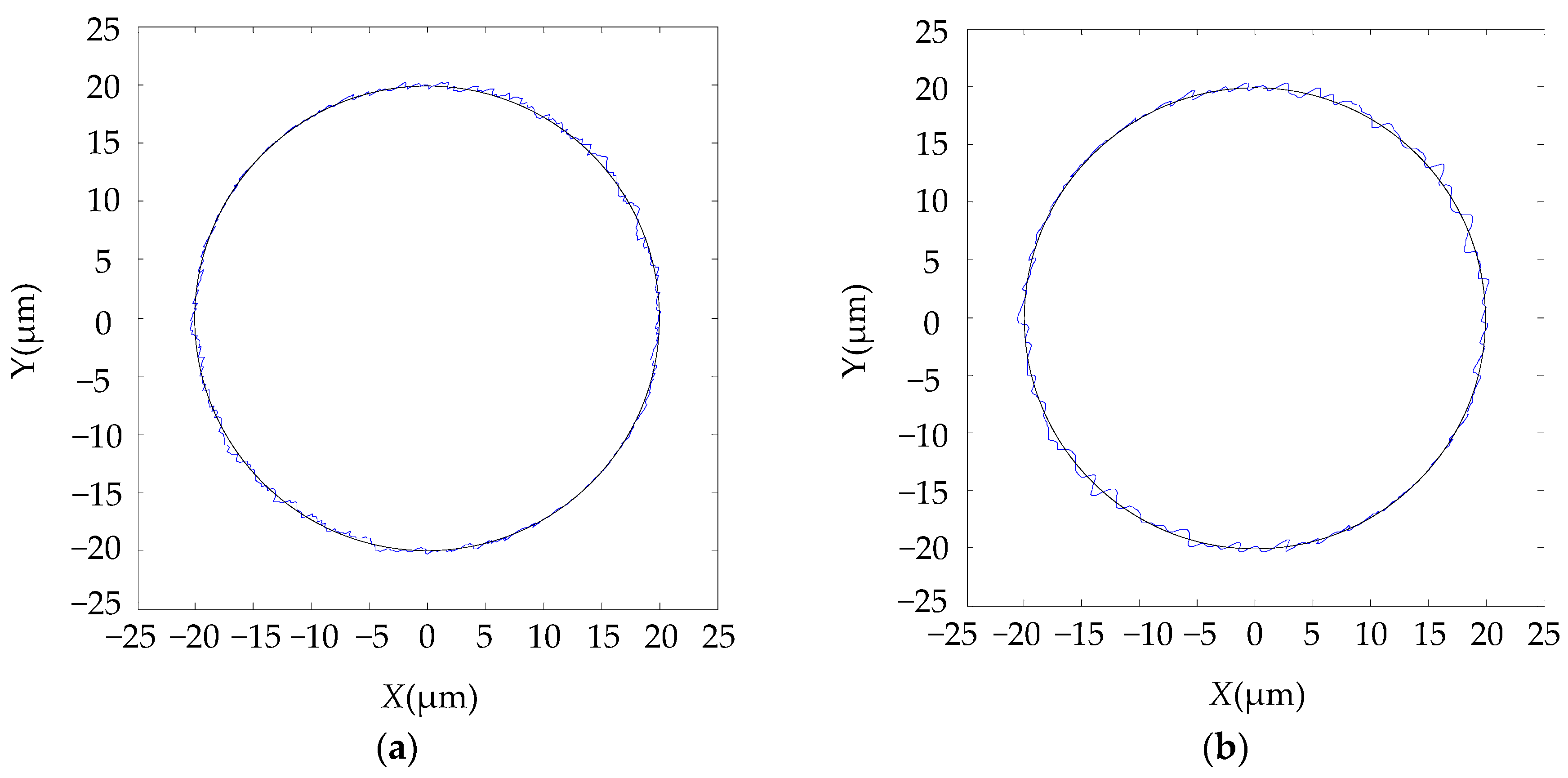
To further compare the anti-disturbance performance of the proposed control strategy and the traditional PID control strategy in terms of the trajectory tracking, a circle reference trajectory is given as the input to both control models. The reference circle trajectory is set in the XY plane with the radius of 20 μm. The random disturbance force with the amplitude of 50 N (half the rated load force) is imposed on both X and Y directions. The simulation result under such random disturbance forces is shown in Figure 10. Figure 10a shows the circle trajectory tracking result for the proposed control model, while Figure 10b shows that for the traditional PID model. It can be seen from Figure 10 that for both control models, the output trajectory can follow the reference circle trajectory. However, the proposed model has better tracking performance because it has less coupling between the X-and Y-axes as analyzed in the 4.3 Decoupling Design.
5.3. System Real-Time Performance Validation
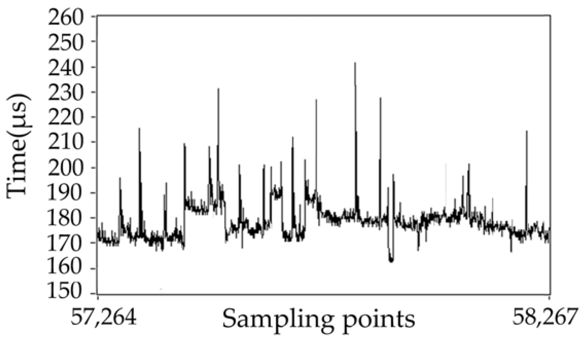
The proposed inverse system-based PID control model has been programmed and run on a NI real-time platform to verify its real-time performance. The real-time control platform consists of an embedded controller, a plug-in I/O module, a PC and a display monitor. The PC connects to the real-time controller via Ethernet cable. The PC is used to design LabVIEW program and download it to the NI controller. NI Controller needs to complete the real-time computation of the program, read data from I/O board and its relevant data is then uploaded to the PC for result visualization. It is common to set a fixed-loop-time for practical industrial control. Within a loop, the output of the controller keeps constant and the controller output changes per fixed-loop-time on average. In most practical real-time industrial applications, the real-time performance requires that the program loop computation time needed is less than 1 ms (or more than 1000 times per second). The fixed program loop time in this test is set to be 200 μs. Figure 11 shows the measured running time needed for each loop. It can be seen that the average run time of the proposed inverse system-based model is close to 200 μs, which indicates that most loops can be completed within the set fixed time period 200 μs. More specifically, the maximum loop run time is 215 μs and the minimum one is 177 μs. Under the fixed mode, the loop will be abandoned if its computation time exceeds the set fixed-loop-time to some extent. To further explore the real computation time for each loop, the above process is replicated under the free-loop-time mode, the result of which is shown in Figure 12. It can be seen form Figure 12 that the average (real) loop time is about 180 μs, with 250 μs and 160 μs as the maximum and minimum loop times, respectively. The test result shows that the proposed control strategy can be used in high-precision industrial applications even taking real-time performance into account.
6. Conclusions
Based on the inverse system method, this paper successfully achieves dynamic decoupling control of an H-shaped platform driven by multiple linear motors, which has multi-variable, nonlinear and coupling characteristics. The inverse system model compensates the original system into a pseudo-linear decoupled linear system, and thus PID controller (typical linear controller) can be used to integrate the control system. To validate the proposed control method, simulation has been done in MATLAB/Simulink to explore the dynamic performance under load force disturbances. The simulation result shows that the displacement deviation between the two linear motors in the Y direction has been controlled to be within a very small range (maximum 0.1 μm) with a recovery time of 0.02 s under the disturbance of half the rated load force, which indicates high synchronization performance. Different from the traditional PID method which controls the X and Y direction movement independently, the proposed inverse system-based PID controller controls the platform mover trajectory in one control system, with the aim to decrease the total positioning error. This has also been validated through the simulation result that the trajectory tracking error under the disturbance of half the rated disturbances is significantly decreased compared with that in the traditional PID method. Extra circle trajectory tracking comparison further validates the above analysis. It indicates that the control system can move along a given reference trajectory under random load disturbance. Furthermore, the designed control system has been run on NI controller under both fixed-loop-time and free-loop-time modes. The result shows the needed loop computation time is about 200 μs, significantly smaller than the required 1 ms in high-precision industrial applications.
In conclusion, the proposed inverse system has high performance for the two main challenges in the control of the H-shaped platform, synchronous deviation and total positioning error. It has also met the real-time requirements, which makes it suitable for real high-precision industrial applications.
Acknowledgments
The main idea of this paper has been conceived since the authors studied in the double master degree EPA (Engineering & Policy Engineering) program between Delft University of Technology and Harbin Institute of Technology, supported by both TU Delft TPM faculty scholarship and Chinese government CSC scholarship.
Author Contributions
All authors have contributed to this article. More specifically, Chaoning Zhang conceived the theoretical analysis and designed the control scheme of the simulation model; Caiyan Qin performed the simulation and performed the real-time performance test. Data processing and analysis were done by Chaoning Zhang and Caiyan Qin. Chaoning Zhang contributed to writing the first draft of this paper and Caiyan Qin took a critical approach to tackle the problems in it and turned it to a complete article. Haiyan Lu was also involved in the research design and helped proofread the paper numerous times.
Conflicts of Interest
The authors declare no conflict of interest.
References
- Rovers, J.M.M.; Jansen, J.W.; Compter, J.C.; Lomonova, E.A. Analysis Method of the Dynamic Force and Torque Distribution in the Magnet Array of a Commutated Magnetically Levitated Planar Actuator. IEEE Trans. Ind. Electron. 2012, 59, 2157–2166. [Google Scholar] [CrossRef]
- Nguyen, V.H.; Kim, J.W. Design and Control of a Compact Lightweight Planar Position Moving over a Concentrated-Field Magnet Matrix. IEEE/ASME Trans. Mechatron. 2013, 18, 1090–1099. [Google Scholar] [CrossRef]
- Wang, L.M.; Tang, Y.P. Fuzzy Cross-coupling Control for Dual Linear Motors based on Preview Feedforward Compensation. In Proceedings of the IEEE International Conference on Mechatronics and Automation, Changchun, China, 9–12 August 2009; pp. 2138–2142. [Google Scholar]
- Koren, Y. Cross-coupled Biaxial Computer Control for Manufacture Systems. ASME J. Dyn. Syst. Meas. Control 1980, 102, 265–272. [Google Scholar] [CrossRef]
- Yan, M.T.; Lee, M.H.; Yen, P.L. Theory and Application of a Combined Self-tuning Adaptive Control and Cross Coupling Control in a Retrofit Milling Machine. Mechatronics 2005, 15, 193–211. [Google Scholar] [CrossRef]
- Lin, F.J.; Hsieh, H.J.; Chou, P.H.; Lin, Y.S. Digital Signal Processor-Based Cross-Coupled Synchronous Control of Dual Linear Motors via Functional Link Radial Basis Function Network. IET Control Theory Appl. 2011, 5, 552–564. [Google Scholar] [CrossRef]
- Shi, R.; Lou, Y.J.; Shao, Y.Q.; Li, J.G.; Chen, H.Y. A Novel Contouring Error Estimation for Position-loop Cross-Coupled Control of Biaxial Servo Systems. In Proceedings of the IEEE/RSJ International Conference on Intelligent Robots and Systems, Daejeon, Korea, 28–30 May 2016; pp. 2197–2202. [Google Scholar]
- Barton, K.L.; Alleyne, A.G. A Cross-Coupled Iterative Learning Control Design for Precision Motion Control. IEEE Trans. Control Syst. Technol. 2008, 16, 1218–1231. [Google Scholar] [CrossRef]
- Sun, D.; Shao, X.; Feng, G. A Model-Free Cross-Coupled Control for Position Synchronization of Multi-Axis Motions: Theory and Experiments. IFAC Proc. Vol. 2005, 38, 1–6. [Google Scholar] [CrossRef]
- Sun, D. Position Synchronization of Multiple Motion Axes with Adaptive Coupling Control. Automatica 2003, 39, 997–1005. [Google Scholar] [CrossRef]
- Sun, D.; Feng, G.; Lam, C.M.; Dong, H. Orientation Control of a Differential Mobile Robot through Wheel Synchronization. IEEE/ASME Trans. Mechatron. 2005, 10, 345–351. [Google Scholar] [CrossRef]
- Zhao, D.; Li, S.; Gao, F.; Zhu, Q. Robust Adaptive Terminal Sliding Mode-Based Synchronized Position Control for Multiple Motion Axed Systems. IET Control Theory Appl. 2009, 3, 136–150. [Google Scholar] [CrossRef]
- Wang, L.M.; Zhang, Z.X.; Li, X.Y. The IT2FNN Synchronous Control for H-type Gantry Stage Driven by Dual Linear Motors. In Proceedings of the 29th Chinese Control and Decision Conference, Chongqing, China, 28–30 May 2017; pp. 4716–4721. [Google Scholar]
- Lin, F.J.; Chou, P.H.; Lin, Y.S. DSP-Based Cross-Coupled Synchronous Control for Dual Linear Motors via Intelligent Complementary Sliding Mode Control. IEEE Trans. Ind. Electron. 2012, 59, 1061–1073. [Google Scholar] [CrossRef]
- Yu, D.M.; Liu, D.; Hu, Q. Synchronous Control for a Dual Linear Motor of Moving Gantry Machining Centers Based on Improved Sliding Mode Variable Structure and Decoupling Control. In Proceedings of the IEEE Control and Decision Conference, Taiyuan, China, 23–25 May 2012; pp. 2525–2528. [Google Scholar]
- Sun, X.D.; Shi, Z.; Chen, L.; Yang, Z.B. Internal Model Control for a Bearingless Permanent Magnet Synchronous Motor Based on Inverse System Method. IEEE Trans. Energy Convers. 2016, 31, 1539–1548. [Google Scholar] [CrossRef]
- Fang, J.C.; Ren, Y. Decoupling Control of Magnetically Suspended Rotor System in Control Moment Gyros Based on an Inverse System Method. IEEE/ASME Trans. Mechatron. 2012, 17, 1133–1144. [Google Scholar] [CrossRef]
- Wang, X.R.; Ma, H. Research on Feedback Linearization Control of Three-Phase Inverter Based on Inverse System. In Proceedings of the IEEE Power Electronics and Motion Control Conference, Harbin, China, 2–5 June 2012; pp. 1353–1357. [Google Scholar]
- Wang, T.S.; Liu, C.C.; Lei, G.; Guo, Y.G.; Zhu, J.G. Model Predictive Direct Torque Control of Permanent Magnet Synchronous Motors with Extended Set of Voltage Space Vectors. IET Electr. Power Appl. 2017, 11, 1376–1382. [Google Scholar] [CrossRef]
- Wang, X.D.; Xia, T.; Xu, X.Z.; Feng, H.C. Design of the Particle Swarm Optimized PID for Permanent Magnet Synchronous Linear Motor. In Proceedings of the IEEE International Conference on Electrical Machines and Systems, Hangzhou, China, 22–25 October 2014; pp. 2289–2293. [Google Scholar]
- Cheema, M.A.M.; Fletcher, J.E.; Rahman, M.F.; Xiao, D. Optimal, Combined Speed, and Direct Thrust Control of Linear Permanent Magnet Synchronous Motors. IEEE Trans. Energy Convers. 2016, 31, 947–958. [Google Scholar] [CrossRef]
Figure 1.
Structure diagram of the H-type platform.

Figure 2.
H-shaped platform force analysis.
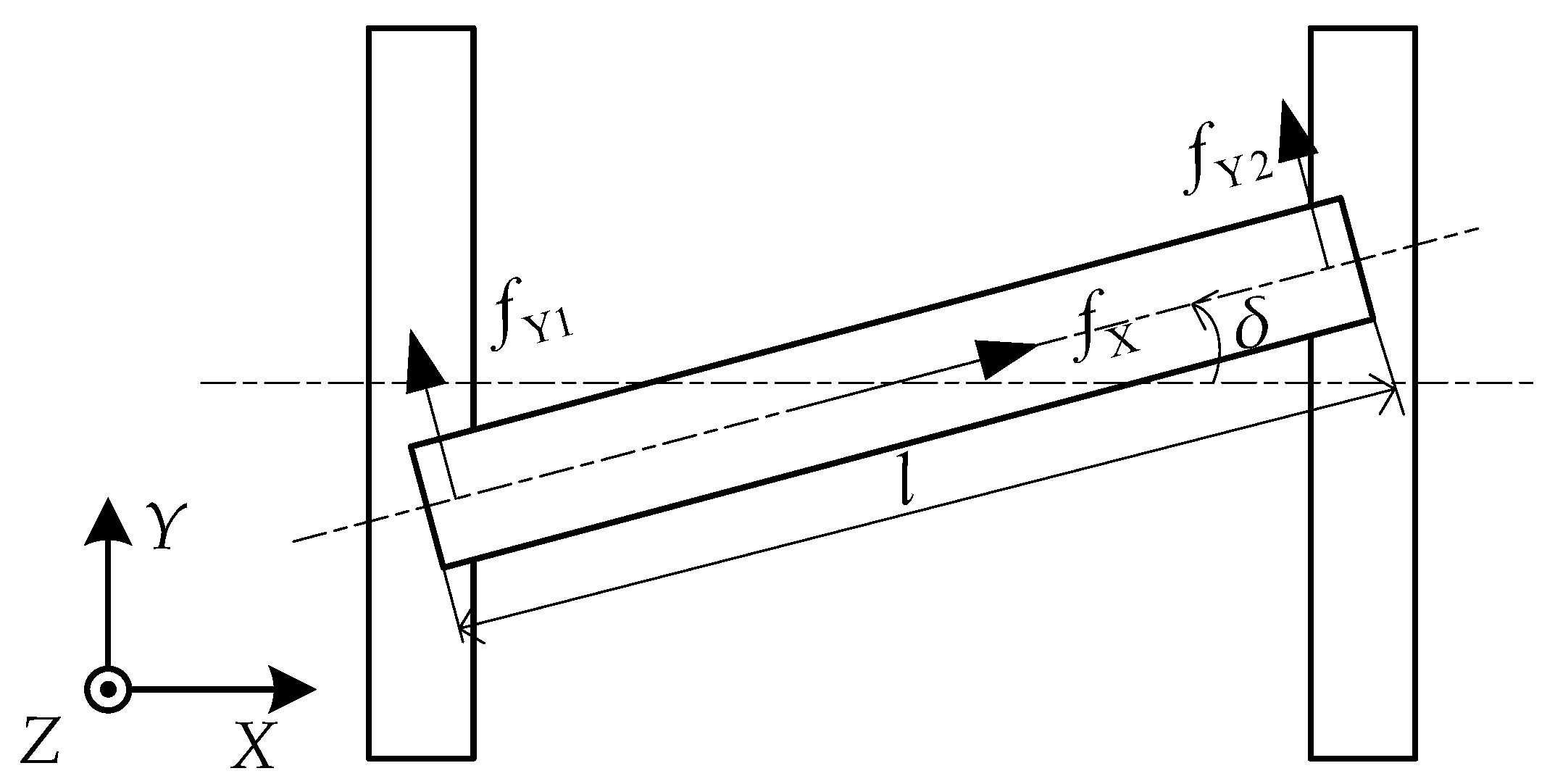
Figure 3.
Structure diagram of PID controller.
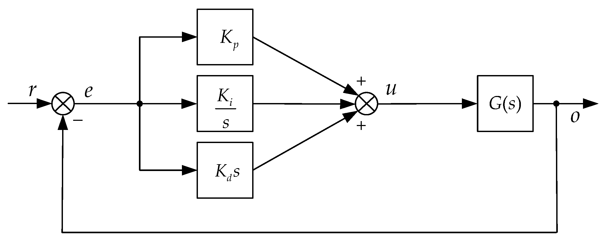
Figure 4.
Decoupled linearization based on α-th order inverse system.

Figure 5.
Control system schematic diagram.

Figure 6.
Y1 Linear Motor: (a) Electromagnetic force; (b) Velocity; (c) Displacement in Y direction.
Figure 6.
Y1 Linear Motor: (a) Electromagnetic force; (b) Velocity; (c) Displacement in Y direction.
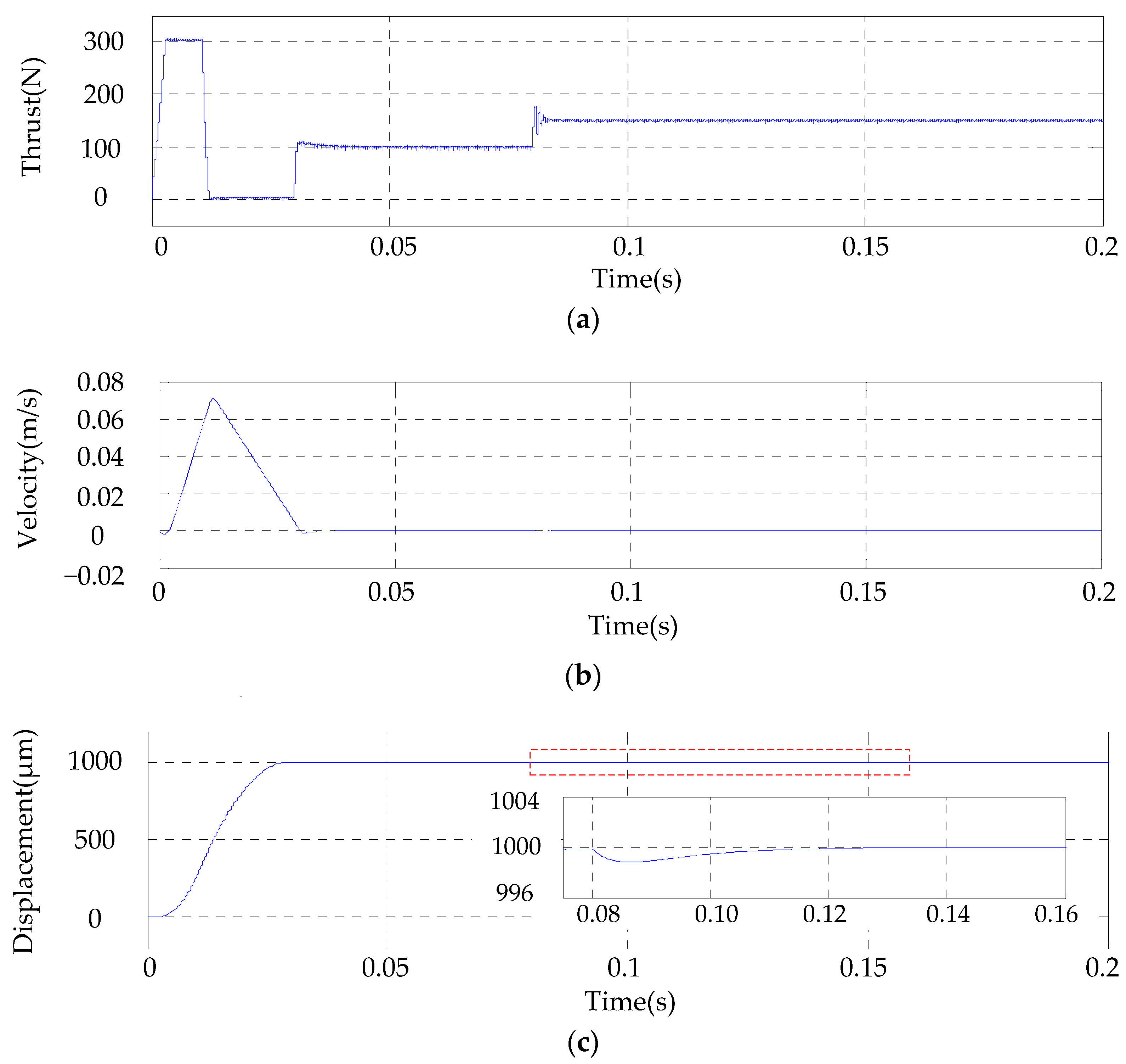
Figure 7.
Y2 Linear Motor: (a)Electromagnetic force; (b) Velocity; (c) Displacement in Y direction.

Figure 8.
Synchronous deviation between Y1 and Y2: (a) disturbance force 20 N; (b) disturbance force 35 N; (c) disturbance force 50 N.
Figure 8.
Synchronous deviation between Y1 and Y2: (a) disturbance force 20 N; (b) disturbance force 35 N; (c) disturbance force 50 N.

Figure 9.
Comparison of platform trajectory: (a) proposed control model based on inverse system; (b) traditional control model.
Figure 9.
Comparison of platform trajectory: (a) proposed control model based on inverse system; (b) traditional control model.
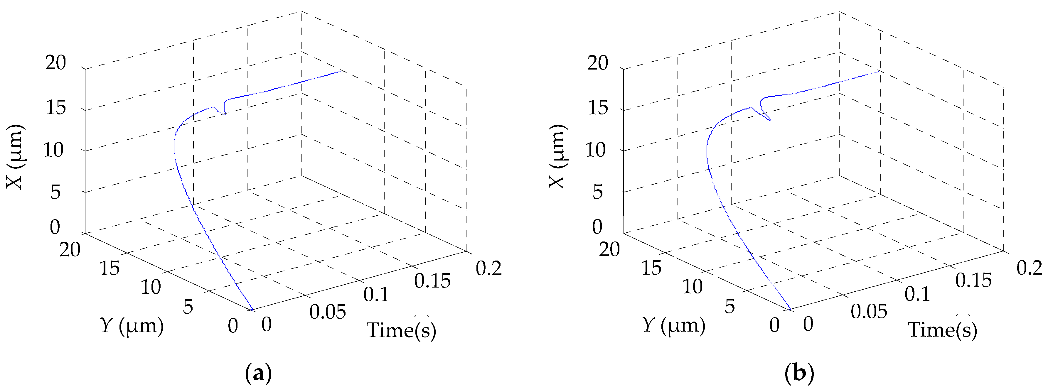
Figure 10.
Circle trajectory tracking analysis: (a) proposed control model; (b) traditional PID control model.
Figure 10.
Circle trajectory tracking analysis: (a) proposed control model; (b) traditional PID control model.

Figure 11.
System run time needed for each computation loop with fixed-loop-time.
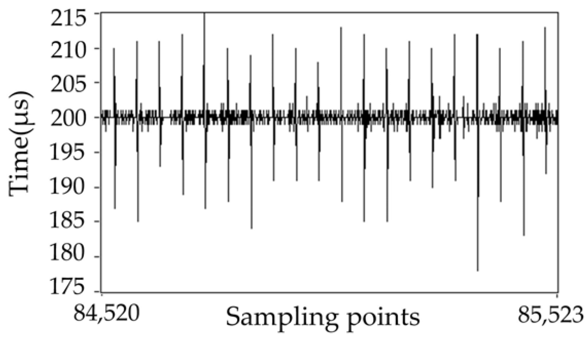
Figure 12.
System run time needed for each computation loop with free-loop-time.


Table 1.
Electromagnetic model parameters.
| Parameter | Value | Unit |
|---|---|---|
| Pole pitch τ | 16 | Mm |
| Flux of permanent magnet ψf | 0.211 | Wb |
| Winding resistance of each phase R | 2.1 | Ω |
| Air gap h | 1 | Mm |
| q-axis inductance Lq | 0.0163 | H |
| d-axis inductance Lq | 0.0163 | H |
| Mass of mover | 0.6 | Kg |
| Rotational inertia J | 0.382 | kg·m2 |
| force arm in Y direction l | 0.42 | M |
© 2017 by the authors. Licensee MDPI, Basel, Switzerland. This article is an open access article distributed under the terms and conditions of the Creative Commons Attribution (CC BY) license (http://creativecommons.org/licenses/by/4.0/).
Share and Cite
MDPI and ACS Style
Qin, C.; Zhang, C.; Lu, H. H-Shaped Multiple Linear Motor Drive Platform Control System Design Based on an Inverse System Method. Energies 2017, 10, 1990. https://doi.org/10.3390/en10121990
AMA Style
Qin C, Zhang C, Lu H. H-Shaped Multiple Linear Motor Drive Platform Control System Design Based on an Inverse System Method. Energies. 2017; 10(12):1990. https://doi.org/10.3390/en10121990
Chicago/Turabian StyleQin, Caiyan, Chaoning Zhang, and Haiyan Lu. 2017. "H-Shaped Multiple Linear Motor Drive Platform Control System Design Based on an Inverse System Method" Energies 10, no. 12: 1990. https://doi.org/10.3390/en10121990
Note that from the first issue of 2016, this journal uses article numbers instead of page numbers. See further details here.