A Novel Method of Statistical Line Loss Estimation for Distribution Feeders Based on Feeder Cluster and Modified XGBoost

1
Key Laboratory of Smart Grid of Ministry of Education, Tianjin University, Tianjin 300072, China
2
State Grid Shanghai Electric Power Research Institute, Shanghai 200437, China
*
Author to whom correspondence should be addressed.
Energies 2017, 10(12), 2067; https://doi.org/10.3390/en10122067
Submission received: 27 October 2017
/
Revised: 22 November 2017
/
Accepted: 26 November 2017
/
Published: 5 December 2017
(This article belongs to the Section F: Electrical Engineering)
Abstract
:The estimation of losses of distribution feeders plays a crucial guiding role for the planning, design, and operation of a distribution system. This paper proposes a novel estimation method of statistical line loss of distribution feeders using the feeder cluster technique and modified eXtreme Gradient Boosting (XGBoost) algorithm that is based on the characteristic data of feeders that are collected in the smart power distribution and utilization system. In order to enhance the applicability and accuracy of the estimation model, k-medoids algorithm with weighting distance for clustering distribution feeders is proposed. Meanwhile, a variable selection method for clustering distribution feeders is discussed, considering the correlation and validity of variables. This paper next modifies the XGBoost algorithm by adding a penalty function in consideration of the effect of the theoretical value to the loss function for the estimation of statistical line loss of distribution feeders. The validity of the proposed methodology is verified by 762 distribution feeders in the Shanghai distribution system. The results show that the XGBoost method has higher accuracy than decision tree, neural network, and random forests by comparison of Root Mean Square Error (RMSE), Mean Absolute Percentage Error (MAPE), and Absolute Percentage Error (APE) indexes. In particular, the theoretical value can significantly improve the reasonability of estimated results.
1. Introduction
Line loss rate is a comprehensive technical and economic index, which reflects the level of planning, design, and operation of power system. It plays a crucial guiding role for optimization of power network structure and saving energy. The loss of 10 kV medium voltage distribution networks accounted for 24.7% of total losses of the power grids, according to the measured result provided by State Grid Corporation of China [1]. That is to say, the line loss of distribution feeders is the heaviest loss layer in the power system. However, the estimation of the losses of distribution feeders becomes a thorny and extensively concerned problem because of the enormous amount of feeders, complicated and variable topologies, and inadequate measuring instruments in the distribution system.
The line loss of distribution system is almost determined by estimation methods that are based on certain hypotheses. The earliest research on loss estimation of a distribution system primarily concentrated on the methods based on load curves and load profile: percent loading [2], statistical features of daily load curves (DLC) [3], and improved statistical representation of the influence of DLCs on power flow of radial distribution networks using average node voltages [4]. The loss factor (LSF) has been extensively applied to calculate the losses of distribution system [5,6,7,8]. Reference [5] estimated the energy losses of distribution system by calculating load variance and load means losses, respectively, using the LSF. Reference [6] proposed loss coefficient (LSC) and equivalent hours of losses (EHL) to replace the LSF and the equivalent hours (EH) for improving the accuracy of energy loss estimation and the applicability of loss patterns. Two formulas of the LSF for calculating energy losses were improved, based on the minimum load factor (MLF) and the load factor (LF) in [7]. Reference [8] proposed an estimation method of technical losses that was based on the reference feeder (RF) of the medium voltage distribution network characterized by LSF, load distribution (LD), feeder peak power demand (PPD), and its length. In order to handle the problem of inadequate information of the distribution system, a top-down/bottom-up method and its improved modus were presented in [9,10,11]. In addition, the clustering technique [12,13], fuzzy logic [14], and decision trees [13] have been applied to improve the accuracy and adaptability of the estimation method. Nevertheless, most of the aforementioned methods have the inherent defects of excessively depending on structure and operation parameters of the distribution system. Although several countermeasures have been proposed to deal with the issue of less available data in distribution systems [9,10,11,12,13,14], it is substantially invalid for the estimation problem of massive, complicated, and diverse distribution feeders. Fortunately, with the development of smart power distribution and utilization system, the comprehensive data that describes the global features of distribution feeders has been preserved, which makes it possible to estimate the statistical line loss of distribution feeders by data mining and machine learning methods.
In this research, eXtreme Gradient Boosting (XGBoost) is selected as the estimation method of statistical line loss of distribution feeders, since it is extensively used by scientific researchers and engineers, and has remarkable performance in many fields, such as energy and remote sensing [15,16,17,18], information technology and software engineering [19,20,21,22], biological and medical engineering [23,24,25], economy, and finance [26,27]. Except for the precise and robust model that is established in XGBoost [28], it is flexible to rewrite the objective function of XGBoost, which makes it possible to estimate statistical line loss with reference to the theoretical value. Meanwhile, in order to improve the applicability and accuracy of the XGBoost model, the thought of clustering distribution feeders [29,30,31] is applied before the estimation procedure.
The rest of this paper is organized as follows. Section 2 presents the full procedure of the estimation of statistical line loss of distribution feeders, including k-medoids algorithm with weighting distance that is used for clustering distribution feeders, and XGBoost model, which is modified by theoretical value for the estimation of statistical line loss. Section 3 details the experimental results and analysis based on real data of 762 feeders. The conclusion is described in Section 4.
2. Materials and Methods
2.1. Data Description and Preprocessing
The dataset selected for this study is from electricity production and operation data in Shanghai. The statistical line loss of distribution feeders and its related data mainly comes from production management system (PMS) and customer management system (CMS). By data extraction and integration, the final dataset used in this study comprises 14 variables, as shown in Table 1. SLLR is a statistical result representing the line loss status, which is calculated by the EES and ES as follows. Correspondingly, the TLLR depicts the line loss by theoretical calculation. Among the affecting factors of statistical line loss in Table 1, EES, ES, and ALRT reflect operation situation of distribution feeders, while TNT, TNL, TRCT, TCLT, TULT, TLL, and PCF are the measures of feeder structure. Meanwhile, ARTT and ARTL are the indirect presentations for operational efficiency of electrical equipment.
The final dataset described in Table 1 is a statistical table of monthly line loss of distribution feeders; moreover, the date of it ranges from August 2015 to September 2016. When considering that the value of the variables of the final dataset fluctuate narrowly and has no significant difference among months, the average value of all the available months are selected as the research data in this study for simplification.
2.2. K-medoids Algorithm with Weighting Distance for Clustering Distribution Feeders
Due to the enormous quantity and various types of distribution feeders, there exists the remarkable difference in topological structure and operation parameters among all of the feeders. Consequently, clustering distribution feeders is proposed as a solution for enhancing the applicability and accuracy of the estimation methodology of statistical line loss. The existing methods that are used for clustering feeders are mainly k-means algorithm [29], k-medoids algorithm [30], and self-organized maps (SOMs) [31]. When considering that there are often certain random perturbations or noise in the line loss dataset of distribution feeders, the k-medoids algorithm is selected as the clustering method for feeders for its insensitivity to the noise and outliers.
2.2.1. Selecting Variables for Clustering Distribution Feeders
Selecting variables for clustering distribution feeders is a process that extracts main factors, which notably distinguish various feeders among multiple influencing factors. Correlation and validity of variables for clustering distribution feeders act as the principle of selecting variables, as follows.
• Correlation of variables for clustering distribution feeders
The clustering result becomes more reasonable and accurate when the cluster variables that are selected are independent of each other. Accordingly, the Pearson correlation coefficient of any two variables is calculated according to the following formula:
where denotes the Pearson correlation coefficient of variable and variable , and are the average of variable and variable , respectively.
• Validity of variables for clustering distribution feeders
The clustering effect of the same variable for different application cases may be significantly different. For example, if the PCF of all the samples in a certain distribution system is close to 1 or changes very little, the effectiveness of it to distinguish the characteristics of distribution feeders seems not remarkable. On the contrary, PCF is supposed to be a crucial factor of clustering distribution feeders when the PCF evidently differs among the entire samples. Based on this fact, the validity of variables for clustering distribution feeders is proposed to quantify this property.
In order to investigate the validity of variables for clustering distribution feeders, the sensitivity of SLLR to every selected variable is calculated, that is, determining the sensitivity coefficient in the Equation (3), as follows:
where is the ith selected variable, is the sensitivity coefficient corresponding to , is the constant term.
Subsequently, the range of each selected variable is calculated by the following equation:
Finally, the validity of variables for clustering distribution feeders is defined as the product of sensitivity coefficient and range of the selected variable as follows:
2.2.2. K-Medoids Algorithm with Weighting Distance
The measurement of the distance between the samples is the foundation of cluster analysis. However, the value of the variables for clustering distribution feeders has significant differences between each other. Moreover, oversimplified and crude normalization will neglect the feature of each variable. Conversely, the aforementioned sensitivity coefficient is capable of reflecting the characteristics of the variables. Consequently, the weighting Euclidean distance is defined as the metric of distance between samples, as follows:
where denotes the distance between the ith sample and the jth sample, and are the kth variable of the ith sample and the jth sample respectively, is the sensitivity coefficient corresponding to the kth variable.
Partitioning Around Medoids (PAM) algorithm is selected as the clustering algorithm for this study, since it is the most common implementation of the k-medoids algorithm. The main steps of PAM is as follows: (1) randomly select k representative objects as initial medoids of the clusters; (2) assign all of the non-selected samples to the closest medoids of the clusters according to the distance function; (3) calculate the total contributions [32] when a representative object is replaced by a non-selected object; and, (4) search the minimal total contributions of all the pairs of representative object and non-selected object; if the minimum is negative, swap the representative object with the non-selected object corresponding to the minimum and the algorithm returns to step 2; otherwise, the algorithm stops. The detailed content of PAM is described in Reference [32].
2.2.3. Determining the Optimal Number of Clusters
The most challenging step in cluster analysis is to determine the optimal number of clusters. There are several theoretical or practical methods that are proposed to handle this problem. Nevertheless, there is no modus that is widely acknowledged and available for entire clustering problems so that a comprehensive strategy is presented by combing with the results of the following four methods in this study.
The sum of squares error (SSE) [33,34] is one of the most common measurements of clustering performance. Evidently, as the number of clusters increases, the size of each cluster becomes smaller and the SSE decreases at the same time. However, it is not necessary to increase the number of clusters when the SSE decreases slowly. Hence, the optimal number of clusters can be determined by observing the relationship between the SSE and the number of clusters.
The Calinski Harabasz index is a widely used cluster validity index to evaluate the partitioning quality [35,36,37,38]. This index is defined as the ratio of the average distance between clusters and average squares error within clusters. Accordingly, the optimal number of clusters can be determined by maximizing the Calinski Harabasz index.
The average silhouette coefficient is a simple but useful index for measuring the result of clustering, and has been applied to many practices [36,37,38,39,40,41]. The core idea of silhouette coefficient is to calculate the difference value of the minimum average distance between a certain sample with samples in other clusters and the average distance within the cluster. Evidently, the higher the average silhouette coefficient, the better.
The hierarchical clustering algorithm [42] is a classical clustering method and performs its capability in lots of clustering problems. A hierarchical and nested clustering tree is constructed in the algorithm by calculating the similarity between the different categories of samples. Consequently, the optimal number of clusters can be determined by visualization of the result of hierarchical clustering.
2.3. XGBoost Algorithm Modified by Theoretical Value for the Estimation of Statistical Line Loss
The XGBoost algorithm [28] is a well-designed Gradient Boosted Decision Tree (GBDT) algorithm [43], which demonstrates its state-of-the-art advantages in the scientific research of machine learning and data mining problem. XGBoost algorithm not only has the advantages of high accuracy of traditional boosting algorithms, but also can deal with sparse data efficiently and implement distributed and parallel computing flexibly. Consequently, the XGBoost algorithm is adaptable to the large-scale dataset.
The XGBoost algorithm achieves an estimate of the target variable by establishing a series of decision trees and assigning each leaf node a quantized weight. The prediction function is as follows:
where is the predictive value of the ith target variable, is the input variable corresponding to , is the total number of the decision trees, is the prediction function corresponding to the kth decision tree and is defined as follows:
where denotes the structure function of the kth decision tree that map to the corresponding leaf node, is the vector of the quantized weight of leaf nodes.
In the XGBoost algorithm, a regularization term is added to the loss function, taking into account the accuracy and complexity of the model at the same time. The set of prediction functions in the model are learned by minimizing the following total loss function:
where denotes the loss function that represents the fitness of the model as a measurement of the differences between the real and predictive values, denotes the complexity of the model. The loss function used in this study is the square loss: . Using to measure the complexity of the model where and are tuning parameters.
When considering the specialty of the estimation of statistical line loss in the power distribution and utilization system that there exists a theoretical value corresponding to each statistical line loss, the prediction of the statistical line loss can be modified by the theoretical line loss. To be specific, the statistical line loss is generally a little bit larger than the theoretical line loss, according to the experience in the operation of the power system. Moreover, there should not be a significant difference between statistical line loss and its theoretical value. Consequently, a penalty function is defined by the utilization of this feature, as follows:
where is the theoretical line loss corresponding to the statistical line loss , and are the parameters for setting the confidence interval of the estimated value, and are the coefficients to regulate the effect of the penalty function.
According to the Equation (10), if , the value of is less than 1. Otherwise, the value of will increase significantly when is far from the interval: . Furthermore, by appropriately tuning the parameters and , the value of could be neglected when in the interval and becomes extremely large while out of the interval. Herein, we set and based on the relationship of statistical line loss and theoretical line loss. Simultaneously, the selected value of and is 0.0001 and 2 respectively. The modified loss function used in this study is as follows:
2.4. The Full Procedure of the Estimation of Statistical Line Loss of Distribution Feeders
The full procedure of the proposed estimation methodology of statistical line loss of distribution feeders is illustrated as follows and presented in Figure 1.
- Feeder cluster. Select variables for clustering distribution feeders by analyzing the correlation and validity of variables, then cluster the input samples using k-medoids algorithm with weighting distance.
- Model training. Determine the model parameters for each cluster by training the XGBoost model that is modified by theoretical value, taking the clustering result, statistical, and theoretical line loss as input data.
- Prediction and evaluation. Predict the statistical line loss in the test set using the aforementioned model and evaluate the performance of the model.
3. Results and Discussion
In our experiment, there are a total number of 762 feeders, including the variables that are described in Table 1, and the software used in this study is R version 3.3.2. The following is the analysis and evaluation of the aforementioned modus.
3.1. Distribution Feeder Cluster
3.1.1. Correlation of Variables for Clustering Distribution Feeders
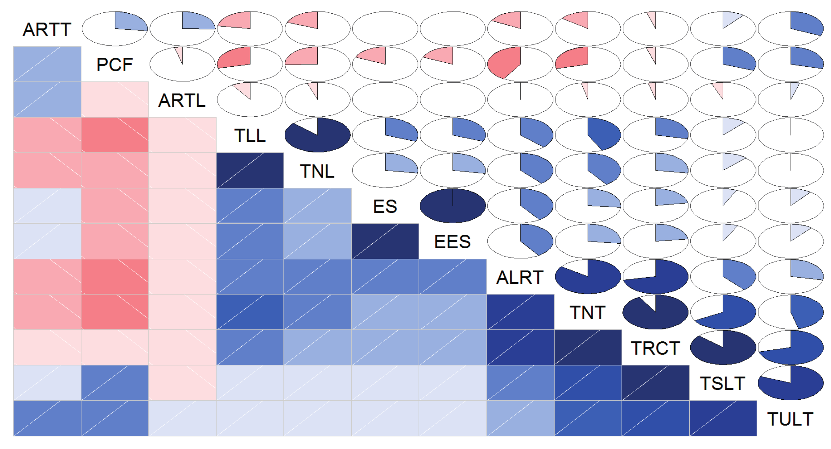
Figure 2 shows the correlation of variables for clustering distribution feeders, according to the Pearson correlation coefficient of any two variables. The lower triangle of Figure 2 (the cells below the principal diagonal of the matrix in Figure 2) denotes the correlation of variables by colors and hashing, where the blue color and the hashing with positive slope represents a positive correlation of the two variables corresponding to the cell, while the red color and the hashing with negative slope expresses the opposite meaning. Furthermore, the colors become darker and more saturated when the value of the correlation is greater. The same information is shown in the upper triangle of Figure 2 using pies. Herein, colors have same meanings, but the magnitude of the correlation is represented by the proportion of the filled pie slice. Moreover, the pie starts at 12 o’clock and moves in a clockwise direction when the correlation of the two variables is positive. Conversely, the pie is filled in a counterclockwise direction indicating the negative correlation [44].
As shown in Figure 2, ARTT, PCF, and ARTL have a weak correlation with other variables. The correlation between TLL and TNL is significantly strong, as is the correlation between EES and ES. Meanwhile, TRCT is positively correlated with ALRT, TNT, TSLT, and TULT. When considering that TLL and TRCT comprise more abundant information than other correlated variables, while EES is easy to measure and more accurate compared with ES, the eliminated variables are TNL, ES, ALRT, TNT, TSLT, and TULT based on correlation analysis.
3.1.2. Validity of Variables for Clustering Distribution Feeders
The sensitivity coefficients in Equation (3) are calculated with the least square method and the range of each selected variable is calculated by Equation (4). Then, the validity of variables for clustering distribution feeders is determined according to the Equation (5), and the result is shown in Table 2. The validity of PCF and ARTL is significantly smaller than that of TRCT, EES, ARTT and TLL, therefore, the variables ultimately selected for clustering distribution feeders are TRCT, EES, ARTT, and TLL.
3.1.3. The Results of Distribution Feeders Cluster with Optimal Number of Clusters
In order to display the effect of weighting distance that is proposed in this study, the variables that are selected for clustering distribution feeders are formatted by multiplying their sensitivity coefficients, as shown in Table 3. There is no significant difference on the scale of all the variables. Hence, the magnitude of a variable has no decisive effect on the measurement of the distance between the two samples. However, the range of each variable is perceptibly different because of the distinct importance of them.
The optimal number of clusters is determined as 2, according to Figure 3. The SSE decreases slowly when the number of clusters is added up to 2 or 4. Furthermore, the Calinski Harabasz index and average silhouette coefficient get maximal value when the number of clusters equals to 2. Meanwhile, according to the dendrogram of hierarchical clustering, two clusters is a reasonable choice for distribution feeders cluster.
The final result of distribution feeder cluster is obtained by the k-medoids algorithm, with weighting distance shown in Table 4. And the sizes of cluster 1 and cluster 2 are 453 and 309, respectively.
3.2. Estimation of Statistical Line Loss of Distribution Feeders
3.2.1. The Evaluation of XGBoost Model for Estimation of Statistical Line Loss
The evaluation indexes used in this study is Root Mean Square Error (RMSE), Mean Absolute Percentage Error (MAPE), and Absolute Percentage Error (APE), as shown in Table 5.
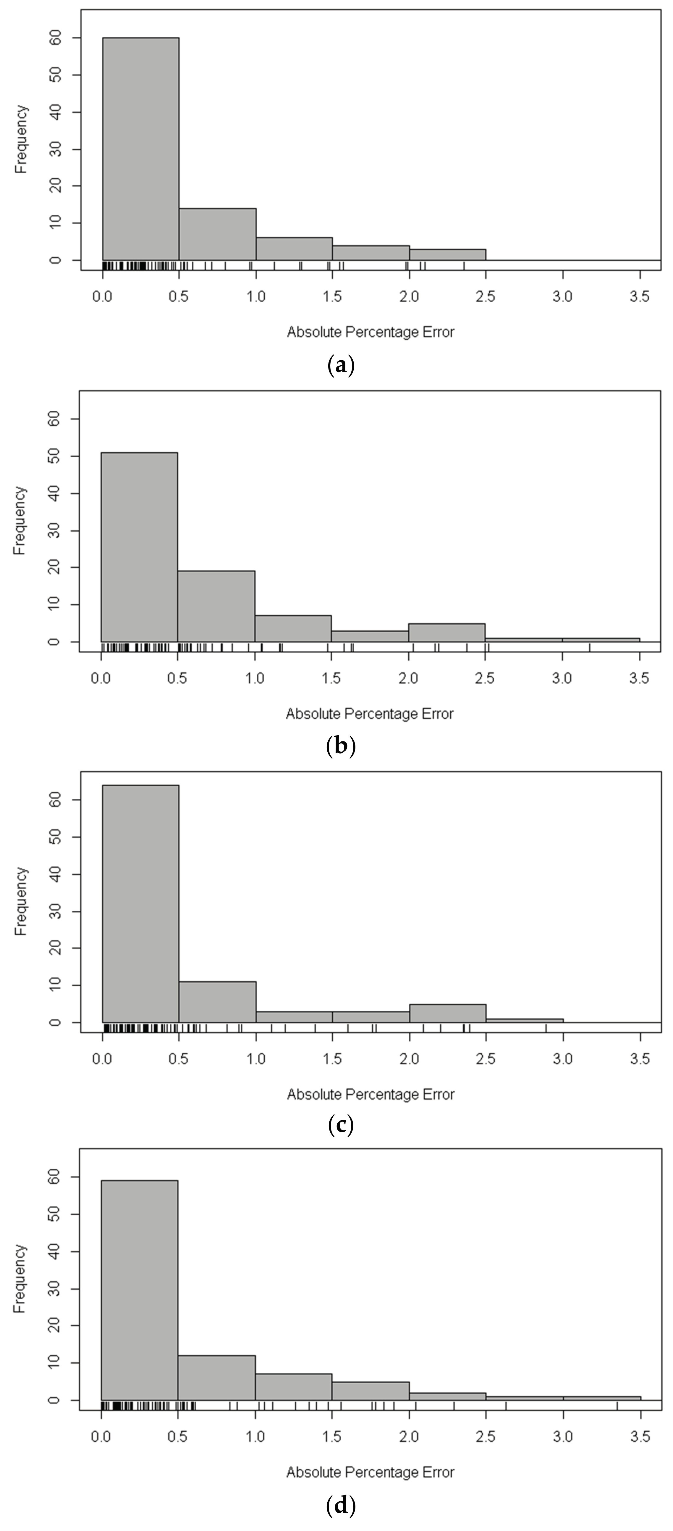
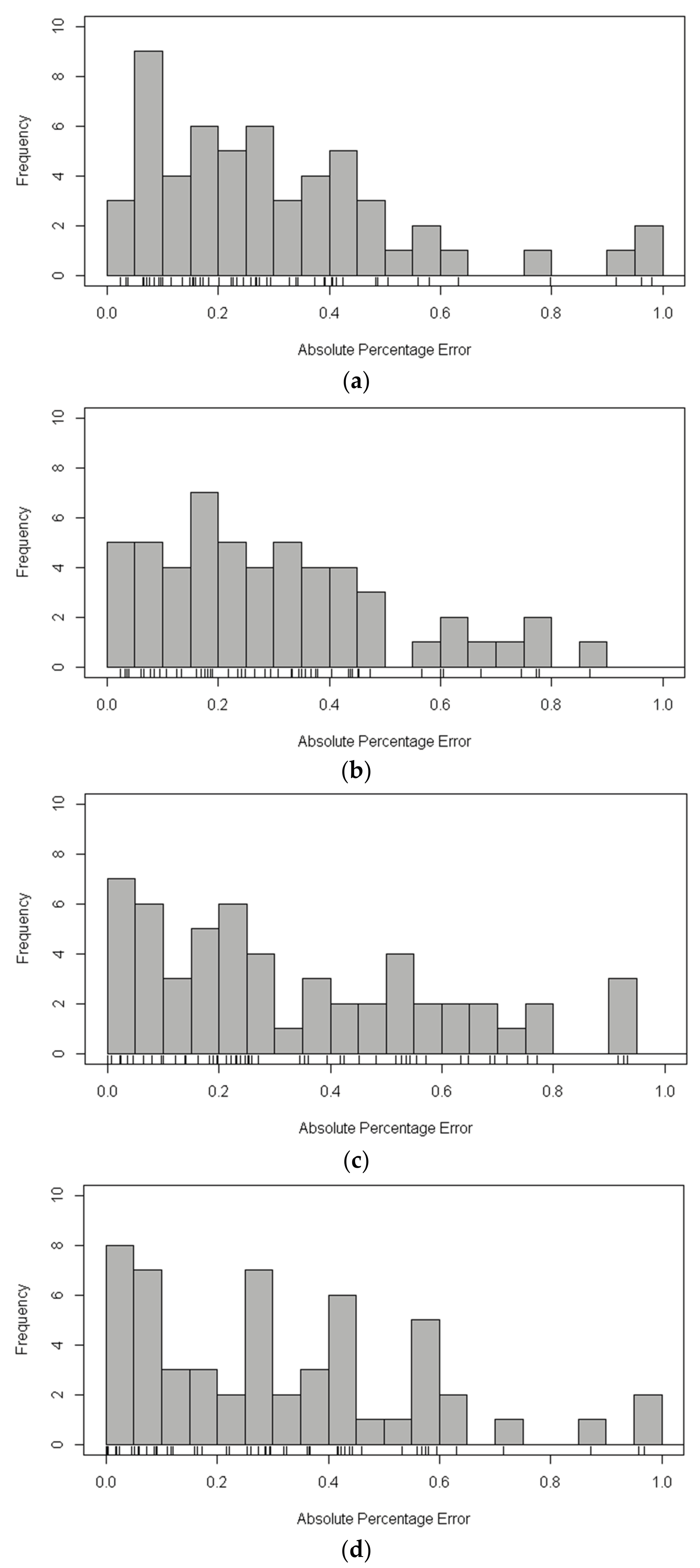
In order to evaluate the performance of XGBoost model for the estimation of statistical line loss, decision tree, neural network, and random forests are selected as a comparison. The implementation of XGBoost, decision tree, neural network, and random forests is by means of R package: XGBoost, rpart, nnet, randomForest, respectively. The dataset that was used in this study is randomly assigned to the training set (80%) and the test set (20%), while the above models are trained using the training set and the models are validated in the test set. The RMSE, MAPE of the estimation results in the test set using aforementioned methods is shown in Table 6. Figure 4 and Figure 5 show the distribution of APE of each sample in the test set by histograms. Moreover, a rug plot [44], which represents the real data values in one-dimensional is added to the plot between bar chart and axis of abscissa to display more detailed information.
In Table 6, the RMSE and MAPE of XGBoost in the test set of both cluster 1 and cluster 2 are the smallest among the four methods. It is worth mentioning that the random forests algorithm has a relatively nice performance since it is a kind of ensemble learning algorithm based on bagging. According to Figure 4, the APE of the XGBoost and random forests algorithm in the test set of cluster 1 mainly concentrated in 0~0.5, while with the increase of APE, the number of samples significantly decreases. However, the frequency of samples has a fluctuation when the APE of the decision tree and neural network algorithm increases. The performance of the four mentioned methods is remarkably different in the test set of cluster 2 when compared with that of cluster 1. As shown in Figure 5, the APE of XGBoost algorithm and the frequency of samples are almost inversely proportional, while the distribution of APE of the other three methods is dispersed and irregular. That is to say, the XGBoost model is more precise and robust.
3.2.2. Estimation of Statistical Line Loss Using XGBoost Model Modified by Theoretical Value
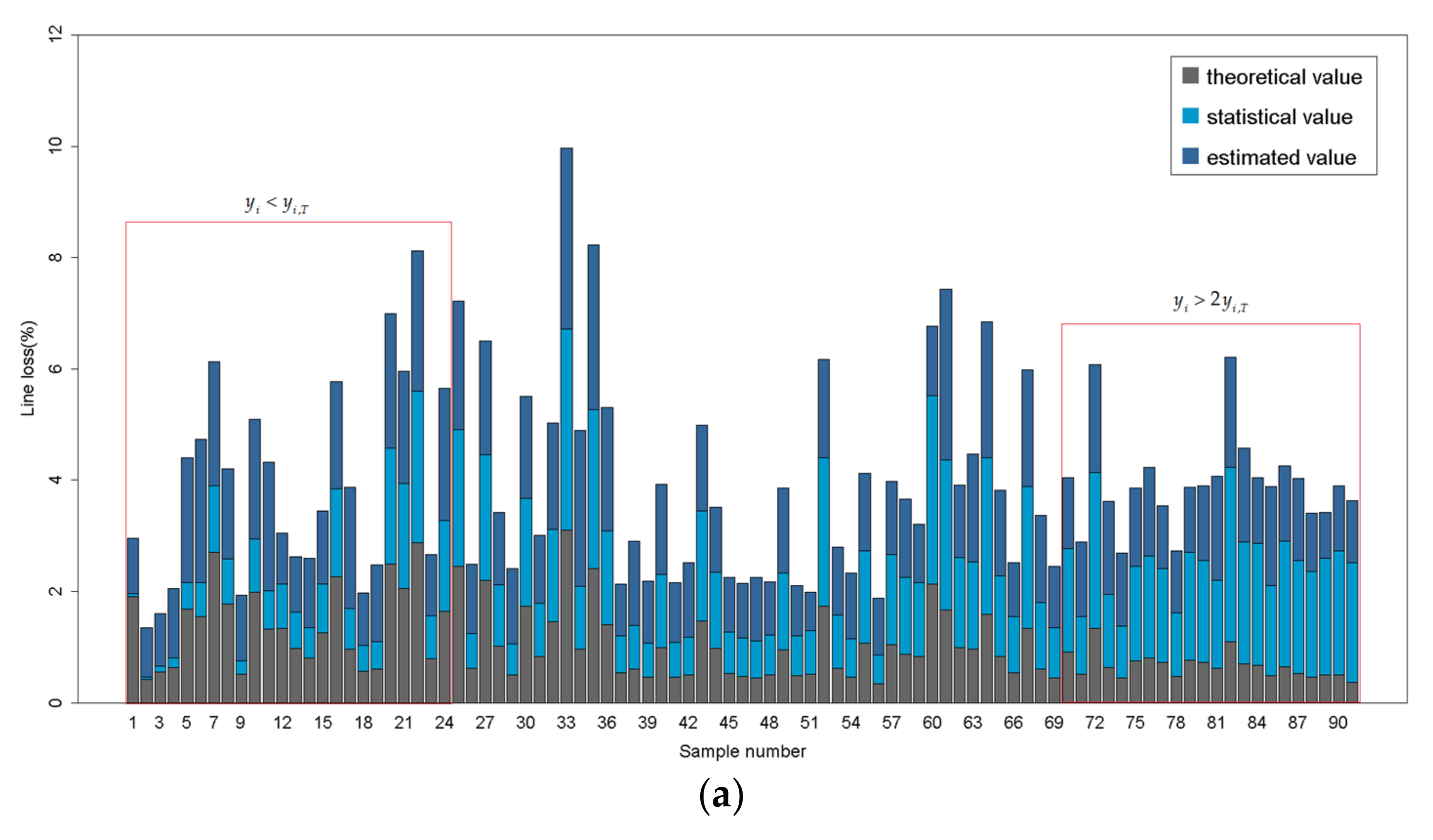
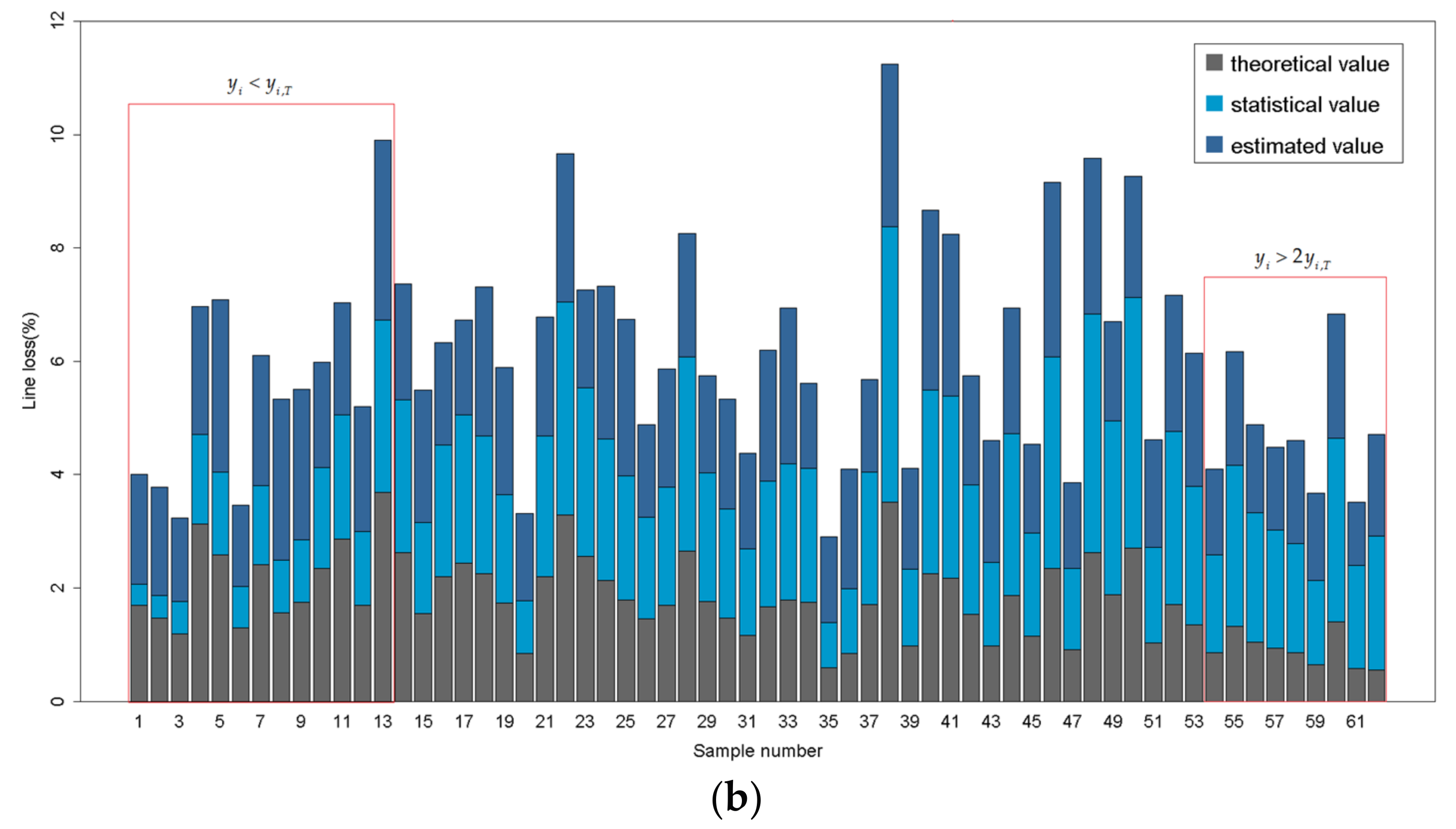
According to Section 2.3, the XGBoost algorithm that is modified by theoretical value is implemented to the estimation of statistical line loss of distribution feeders. Likewise, the dataset is randomly assigned to the training set (80%) for training the model and the test set (20%) for model validation. Figure 6 shows the estimated value, statistical value and theoretical value in the test set by means of a histogram. The samples are numbered in the order of the relative difference between statistical value and theoretical value: . As shown in Figure 6, when or , the estimated value is obtained based on both the statistical value and theoretical value. Moreover, the estimated value is more dependent on the theoretical value when the statistical value becomes farther from the reasonable scope.
Our experiment is conducted on a computer with 2.40 GHz Intel(R) Core(TM) i5-2430 M CPU, 6 GB RAM, and Microsoft Windows 7 Ultimate with Service Pack 1 (x64) operating system. The computation time of the model training procedure in the original XGBoost algorithm for cluster 1 and cluster 2 are 226 ms and 151 ms, respectively. The time in the modified XGBoost algorithm are 270 ms and 186 ms for each cluster. Meanwhile, the computation time of the estimation procedure in both the original XGBoost algorithm and the modified XGBoost algorithm is approximately 0.1 ms. That is, the efficiency of the modified XGBoost is slightly lower than the original XGBoost so the nice performance of XGBoost [28] is maintained in the modified method. In addition, the model training procedure is based on a great amount of historical data so that it is usually performed by off-line computation and is updated periodically. The estimation procedure meets the requirement of on-line computation, and can be used for both on line and off line.
4. Conclusions
A novel estimation method of statistical line loss of distribution feeders using feeder cluster technique and modified XGBoost algorithm is proposed. The principal novelty of the estimation model proposed is to enhance the reasonability of estimated results of statistical line loss by considering the auxiliary function of the theoretical line loss. According to the estimated result, as shown in Figure 6, the theoretical value is capable of amending the estimated value when the statistical value is beyond reasonable interval. Moreover, it is substantially common that the statistical line loss is incorrect in the real data of distribution system. Accordingly, the estimation method that is proposed in this study is applicable to the amendment of the lost data and abnormal data of statistical line loss of distribution feeders. Except for that, the ideology of improving the performance of the numerical estimation model by the application of professional knowledge can be extended to other fields.
The procedure of selecting variables for clustering distribution feeders is verified to be effective in this study and can be applied to any other feeder classification problems according to the specific application purpose. Meanwhile, the weighting distance based on the sensitivity coefficient is better than the oversimplified and crude normalization for considering specific characteristics of each variable.
The estimation method, as based on XGBoost, outperforms traditional machine learning algorithms methods, such as decision tree, neural network, and random forests in terms of RMSE, MAPE, and APE indexes. Nevertheless, the parameters of XGBoost model are manually and empirically tuned in this study. Therefore, better performance can be obtained by optimizing the tuning parameters using Bayesian [27], genetic algorithms [45], and any other methods in future works.
Acknowledgments
This work was supported by the National High Technology Research and Development Program of China (Grant No. 2015AA050203).
Author Contributions
All the authors have participated to the design of experiments, analysis of data and results, and writing of the paper.
Conflicts of Interest
The authors declare no conflict of interest.
References
- Yu, W.; Xiong, Y.; Zhou, X.; Zhao, G.; Chen, N. Analysis on technical line losses of power grids and countermeasures to reduce line losses. Power Syst. Technol. 2006, 30, 54–57. [Google Scholar] [CrossRef]
- Flaten, D.L. Distribution system losses calculated by percent loading. IEEE Trans. Power Syst. 1988, 3, 1263–1269. [Google Scholar] [CrossRef]
- Shenkman, A.L. Energy loss computation by using statistical techniques. IEEE Trans. Power Deliv. 1990, 5, 254–258. [Google Scholar] [CrossRef]
- Taleski, R.; Rajicic, D. Energy summation method for energy loss computation in radial distribution networks. IEEE Trans. Power Syst. 1996, 11, 1104–1111. [Google Scholar] [CrossRef]
- Mikic, O.M. Variance-based energy loss computation in low voltage distribution networks. IEEE Trans. Power Syst. 2007, 22, 179–187. [Google Scholar] [CrossRef]
- Queiroz, L.M.O.; Roselli, M.A.; Cavellucci, C.; Lyra, C. Energy losses estimation in power distribution systems. IEEE Trans. Power Syst. 2012, 27, 1879–1887. [Google Scholar] [CrossRef]
- Fu, X.; Chen, H.; Cai, R.; Xuan, P. Improved LSF method for loss estimation and its application in DG allocation. IET Gener. Transm. Distrib. 2016, 10, 2512–2519. [Google Scholar] [CrossRef]
- Ibrahim, K.A.; Au, M.T.; Gan, C.K.; Tang, J.H. System wide MV distribution network technical losses estimation based on reference feeder and energy flow model. Int. J. Electr. Power Energy Syst. 2017, 93, 440–450. [Google Scholar] [CrossRef]
- Dortolina, C.; Nadira, R. The loss that is unknown is no loss at all: A top-down/bottom-up approach for estimating distribution losses. IEEE Trans. Power Syst. 2005, 20, 1119–1125. [Google Scholar] [CrossRef]
- Oliveira, M.E.; Padilha-Feltrin, A. A top-down approach for distribution loss evaluation. IEEE Trans. Power Deliv. 2009, 24, 2117–2124. [Google Scholar] [CrossRef]
- Armaulia Sanchez, V.; Lima, D.A.; Ochoa, L.F.; Oliveira, M.E. Statistical Top-Down Approach for Energy Loss Estimation in Distribution Systems. In Proceedings of the 2015 IEEE Eindhoven Powertech, Eindhoven, The Netherlands, 29 June–2 July 2015. [Google Scholar]
- Dashtaki, A.K.; Haghifam, M.R. A new loss estimation method in limited data electric distribution networks. IEEE Trans. Power Deliv. 2013, 28, 2194–2200. [Google Scholar] [CrossRef]
- Grigoras, G.; Scarlatache, F. Energy Losses Estimation in Electrical Distribution Networks with a Decision Trees-based Algorithm. In Proceedings of the 2013 8th International Symposium on Advanced Topics in Electrical Engineering (ATEE), Bucharest, Romania, 23–25 May 2013. [Google Scholar]
- Lezhniuk, P.; Bevz, S.; Piskliarova, A. Evaluation and Forecast of Electric Energy Losses in Distribution Networks Applying Fuzzy-Logic. In Proceedings of the 2008 IEEE Power & Energy Society General Meeting, Pittsburgh, PA, USA, 20–24 July 2008; Volumes 1–11, pp. 3279–3282. [Google Scholar]
- Zheng, H.; Yuan, J.; Chen, L. Short-term load forecasting using EMD-LSTM neural networks with a Xgboost algorithm for feature importance evaluation. Energies 2017, 10, 1168. [Google Scholar] [CrossRef]
- Urraca, R.; Martinez-de-Pison, E.; Sanz-Garcia, A.; Antonanzas, J.; Antonanzas-Torres, F. Estimation methods for global solar radiation: Case study evaluation of five different approaches in central Spain. Renew. Sustain. Energy Rev. 2017, 77, 1098–1113. [Google Scholar] [CrossRef]
- Chen, W.; Fu, K.; Zuo, J.; Zheng, X.; Huang, T.; Ren, W. Radar emitter classification for large data set based on weighted-xgboost. IET Radar Sonar Navig. 2017, 11, 1203–1207. [Google Scholar] [CrossRef]
- Aler, R.; Galvan, I.M.; Ruiz-Arias, J.A.; Gueymard, C.A. Improving the separation of direct and diffuse solar radiation components using machine learning by gradient boosting. Sol. Energy 2017, 150, 558–569. [Google Scholar] [CrossRef]
- Baker, J.; Pomykalski, A.; Hanrahan, K.; Guadagni, G. Application of Machine Learning Methodologies to Multiyear Forecasts of Video Subscribers. In Proceedings of the 2017 Systems and Information Engineering Design Symposium (SIEDS), Charlottesville, VA, USA, 28 April 2017; pp. 100–105. [Google Scholar]
- Ge, Y.; He, S.; Xiong, J.; Brown, D.E. Customer Churn Analysis for a Software-as-a-service Company. In Proceedings of the 2017 Systems and Information Engineering Design Symposium (SIEDS), Charlottesville, VA, USA, 28 April 2017; pp. 106–111. [Google Scholar]
- Zhang, Y.; Huang, Q.; Ma, X.; Yang, Z.; Jiang, J. Using Multi-features and Ensemble Learning Method for Imbalanced Malware Classification. In Proceedings of the 2016 IEEE Trustcom/BigDataSE/ISPA, Tianjin, China, 23–26 August 2016; pp. 965–973. [Google Scholar]
- Ayumi, V. Pose-based Human Action Recognition with Extreme Gradient Boosting. In Proceedings of the 14th IEEE Student Conference on Research and Development (SCORED), Kuala Lumpur, Malaysia, 13–14 December 2016. [Google Scholar]
- Lei, T.; Chen, F.; Liu, H.; Sun, H.; Kang, Y.; Li, D.; Li, Y.; Hou, T. ADMET evaluation in drug discovery. Part 17: Development of quantitative and qualitative prediction models for chemical-induced respiratory toxicity. Mol. Pharm. 2017, 14, 2407–2421. [Google Scholar] [CrossRef] [PubMed]
- Mustapha, I.B.; Saeed, F. Bioactive molecule prediction using extreme gradient boosting. Molecules 2016, 21, 983. [Google Scholar] [CrossRef] [PubMed]
- Sheridan, R.P.; Wang, W.M.; Liaw, A.; Ma, J.; Gifford, E.M. Extreme gradient boosting as a method for quantitative structure-activity relationships. J. Chem. Inf. Model. 2016, 56, 2353–2360. [Google Scholar] [CrossRef] [PubMed]
- Xia, Y.; Liu, C.; Li, Y.; Liu, N. A boosted decision tree approach using Bayesian hyper-parameter optimization for credit scoring. Expert Syst. Appl. 2017, 78, 225–241. [Google Scholar] [CrossRef]
- Xia, Y.; Liu, C.; Liu, N. Cost-sensitive boosted tree for loan evaluation in peer-to-peer lending. Electron. Commer. Res. Appl. 2017, 24, 30–49. [Google Scholar] [CrossRef]
- Chen, T.; Guestrin, C. XGBoost: A scalable tree boosting system. In Proceedings of the ACM SIGKDD International Conference on Knowledge Discovery and Data Mining, San Francisco, CA, USA, 13–17 August 2016; pp. 785–794. [Google Scholar]
- Broderick, R.J.; Williams, J.R. Clustering Methodology for Classifying Distribution Feeders. In Proceedings of the 2013 IEEE 39th Photovoltaic Specialists Conference (PVSC), Tampa, FL, USA, 16–21 June 2013; pp. 1706–1710. [Google Scholar]
- Cale, J.; Palmintier, B.; Narang, D.; Carroll, K. Clustering Distribution Feeders in the Arizona Public Service Territory. In Proceedings of the 2014 IEEE 40th Photovoltaic Specialist Conference (PVSC), Denver, CO, USA, 8–13 June 2014; pp. 2076–2081. [Google Scholar]
- Dehghani, F.; Dehghani, M.; Nezami, H.; Saremi, M. Distribution Feeder Classification Based on Self Organized Maps (Case Study: Lorestan Province, Iran). In Proceedings of the 2015 20th Conference on Electrical Power Distribution Networks Conference (EPDC), Zahedan, Iran, 28–29 April 2015; pp. 27–31. [Google Scholar]
- Van der Laan, M.; Pollard, K.; Bryan, J. A new partitioning around medoids algorithm. J. Stat. Comput. Simul. 2003, 73, 575–584. [Google Scholar] [CrossRef]
- Kwedlo, W. A clustering method combining differential evolution with the K-means algorithm. Pattern Recognit. Lett. 2011, 32, 1613–1621. [Google Scholar] [CrossRef]
- Kishor, D.R.; Venkateswarlu, N.B. A Behavioral Study of Some Widely Employed Partitional and Model-Based Clustering Algorithms and Their Hybridizations. In Advances in Intelligent Systems and Computing, Proceedings of the International Conference on Data Engineering and Communication Technology, (ICDECT 2016) Volume 2, Pune, India, 10–11 March 2016; Satapathy, S.C., Bhateja, V., Joshi, A., Eds.; Springer: Singapore, 2017; Volume 469, pp. 587–601. [Google Scholar]
- Maulik, U.; Bandyopadhyay, S. Performance evaluation of some clustering algorithms and validity indices. IEEE Trans. Pattern Anal. Mach. Intell. 2002, 24, 1650–1654. [Google Scholar] [CrossRef]
- Schepers, J.; Ceulemans, E.; Van Mechelen, I. Selecting among multi-mode partitioning models of different complexities: A comparison of four model selection criteria. J. Classif. 2008, 25, 67–85. [Google Scholar] [CrossRef]
- De Amorim, R.C.; Hennig, C. Recovering the number of clusters in data sets with noise features using feature rescaling factors. Inf. Sci. 2015, 324, 126–145. [Google Scholar] [CrossRef] [Green Version]
- Lord, E.; Willems, M.; Lapointe, F.-J.; Makarenkov, V. Using the stability of objects to determine the number of clusters in datasets. Inf. Sci. 2017, 393, 29–46. [Google Scholar] [CrossRef]
- Chiang, M.M.-T.; Mirkin, B. Intelligent choice of the number of clusters in k-means clustering: An experimental study with different cluster spreads. J. Classif. 2010, 27, 3–40. [Google Scholar] [CrossRef]
- Mur, A.; Dormido, R.; Duro, N.; Dormido-Canto, S.; Vega, J. Determination of the optimal number of clusters using a spectral clustering optimization. Expert Syst. Appl. 2016, 65, 304–314. [Google Scholar] [CrossRef]
- Martinez-Penaloza, M.-G.; Mezura-Montes, E.; Cruz-Ramirez, N.; Acosta-Mesa, H.-G.; Rios-Figueroa, H.-V. Improved multi-objective clustering with automatic determination of the number of clusters. Neural Comput. Appl. 2017, 28, 2255–2275. [Google Scholar] [CrossRef]
- Langfelder, P.; Zhang, B.; Horvath, S. Defining clusters from a hierarchical cluster tree: The Dynamic Tree Cut package for R. Bioinformatics 2008, 24, 719–720. [Google Scholar] [CrossRef] [PubMed]
- Friedman, J. Greedy function approximation: A gradient boosting machine. Ann. Stat. 2001, 29, 1189–1232. [Google Scholar] [CrossRef]
- Kabacoff, R. R in Action, 2nd ed.; Shelter Island: New York, NY, USA, 2015; pp. 125–127, 271–276. [Google Scholar]
- Javier Martinez-de-Pison, F.; Fraile-Garcia, E.; Ferreiro-Cabello, J.; Gonzalez, R.; Pernia, A. Searching Parsimonious Solutions with GA-PARSIMONY and XGBoost in High-Dimensional Databases. In Advances in Intelligent Systems and Computing, Proceedings of the International Joint Conference SOCO’16-CISIS’16-ICEUTE’16, Saint Sebastian, Spain, 19–21 October 2016; Grana, M., LopezGuede, J.M., Etxaniz, O., Herrero, A., Quintian, H., Corchado, E., Eds.; Springer: Cham, Switzerland, 2017; Volume 527, pp. 201–210. [Google Scholar]
Figure 1.
The flowchart of the estimation method of statistical line loss of distribution feeders.
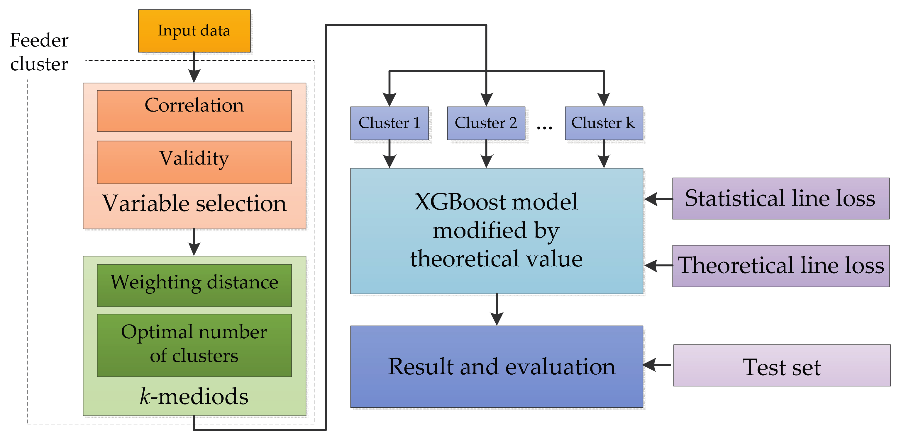
Figure 2.
The Correlation graph of variables for clustering distribution feeders.

Figure 3.
The scheme of selecting an optimal number of clusters. (a) The sum of squares error corresponding to the number of clusters; (b) The average silhouette coefficient corresponding to the number of clusters; (c) The Calinski Harabasz index corresponding to the number of clusters; and, (d) The result of hierarchical clustering.
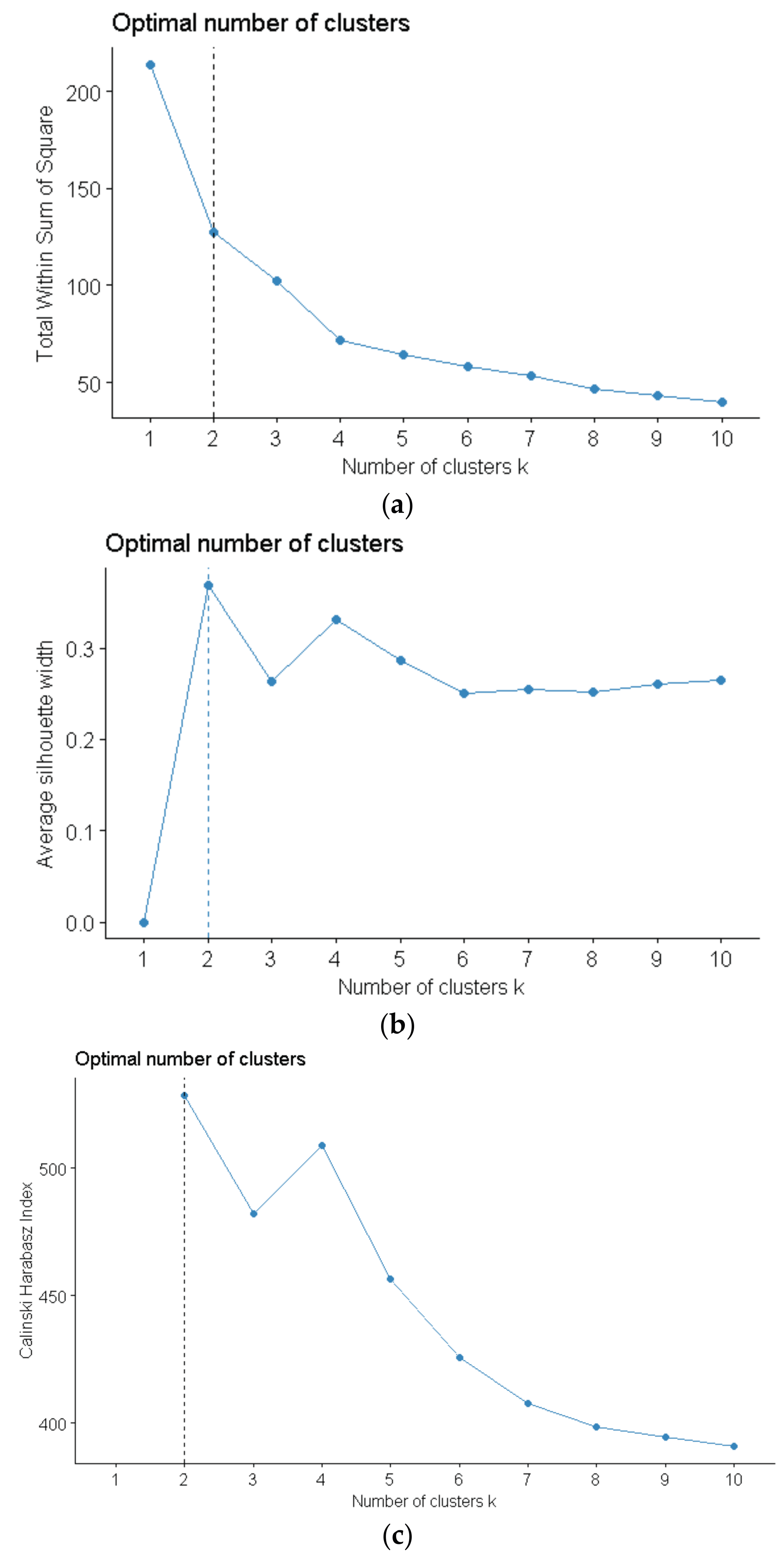
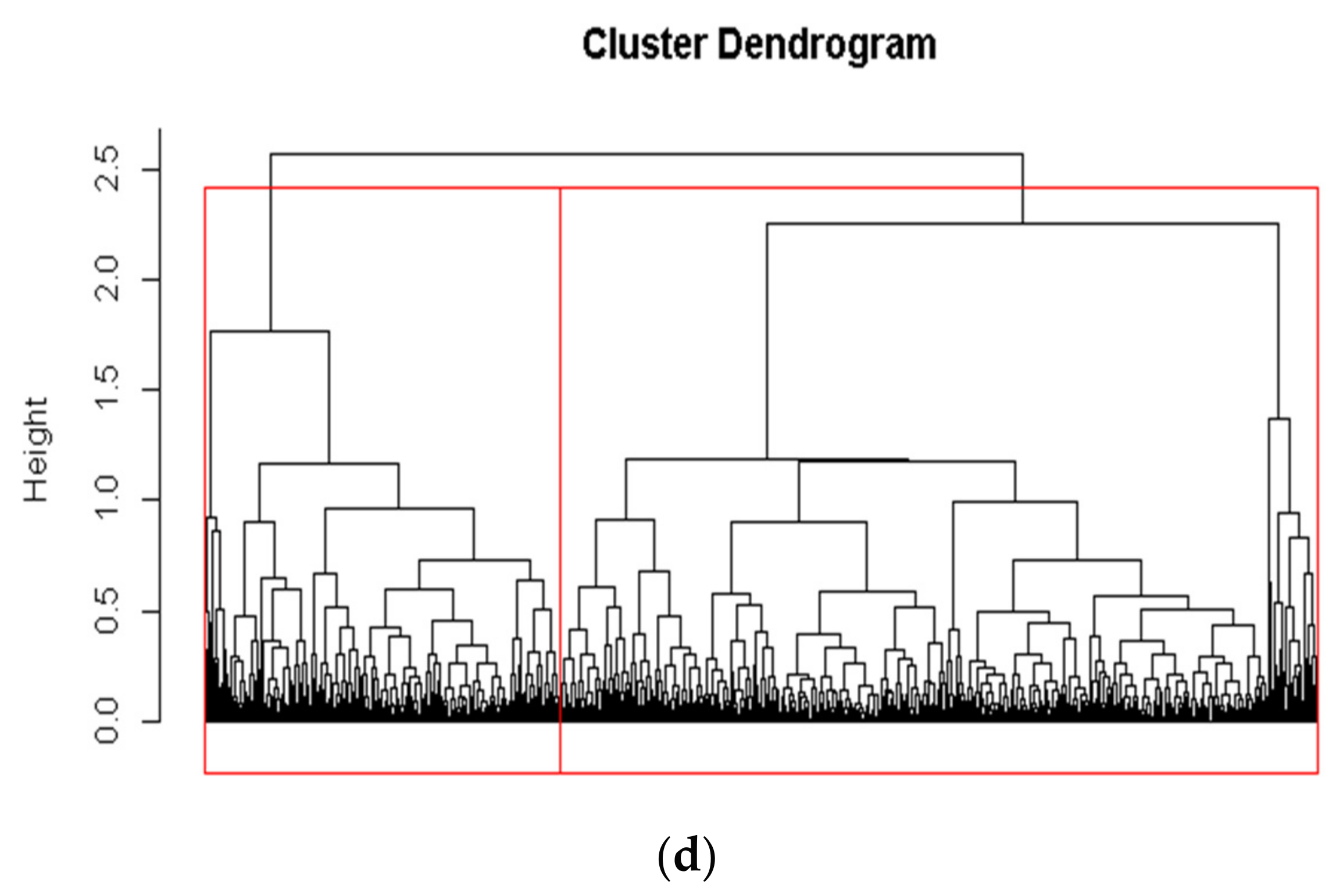
Figure 4.
The distribution of Absolute Percentage Error (APE) of each sample in the test set of cluster 1. (a) The distribution of APE using eXtreme Gradient Boosting (XGBoost); (b) The distribution of APE using decision tree; (c) The distribution of APE using neural network; and, (d) The distribution of APE using random forests.

Figure 5.
The distribution of APE of each sample in the test set of cluster 2. (a) The distribution of APE using XGBoost; (b) The distribution of APE using decision tree; (c) The distribution of APE using neural network; and, (d) The distribution of APE using random forests.
Figure 5.
The distribution of APE of each sample in the test set of cluster 2. (a) The distribution of APE using XGBoost; (b) The distribution of APE using decision tree; (c) The distribution of APE using neural network; and, (d) The distribution of APE using random forests.

Figure 6.
The histogram of the estimated value, statistical value and theoretical value in the test set. (a) The estimated value, statistical value and theoretical value in the test set of cluster 1; (b) The estimated value, statistical value and theoretical value in the test set of cluster 2.
Figure 6.
The histogram of the estimated value, statistical value and theoretical value in the test set. (a) The estimated value, statistical value and theoretical value in the test set of cluster 1; (b) The estimated value, statistical value and theoretical value in the test set of cluster 2.

Table 1.
Description of the variables of the final dataset used in this study.
| Variables | Description | Variables | Description |
|---|---|---|---|
| SLLR | Statistical Line Loss Rate of a Feeder | TLLR | Theoretical Line Loss Rate of a feeder |
| EES | Electrical Energy Supply of a Feeder | ES | Electricity Sales Belonging to a Feeder |
| TNT | Total Number of Transformers Belonging to a Feeder | TRCT | Total Rated Capacity of Transformers Belonging to a Feeder |
| TSLT | Total Short Circuit Loss of Transformers Belonging to a Feeder | TULT | Total Unload Loss of Transformers Belonging to a Feeder |
| ALRT | Average Load Rate of Transformers Belonging to a Feeder | ARTT | Average Run Time of Transformers Belonging to a Feeder |
| TNL | Total Number of Lines Belonging to a Feeder | TLL | Total Length of Lines Belonging to a Feeder |
| PCF | Proportion of Cable in a Feeder | ARTL | Average Run Time of Lines Belonging to a Feeder |
Table 2.
The result of validity of variables for clustering distribution feeders.
| Indexes | TRCT (kW) | EES (kWh) | ARTT (m) | TLL (m) | PCF | ARTL (m) |
|---|---|---|---|---|---|---|
| 1.11 × 10⁻⁴ | 7.81 × 10⁻⁷ | 4.21 × 10⁻³ | 1.26 × 10⁻⁵ | 6.51 × 10⁻² | 1.76 × 10⁻⁵ | |
| 20,440.0 | 2,830,644.8 | 240.0 | 26,846.0 | 1.0 | 656.5 | |
| 2.271 | 2.210 | 1.010 | 0.337 | 0.065 | 0.011 |
Table 3.
The quantiles of formatted variables for clustering distribution feeders.
| Quantiles | TRCT | EES | ARTT | TLL |
|---|---|---|---|---|
| Minimum | 0.01109 | 0.00867 | 0.00414 | 0.00070 |
| 1st Quantile | 0.17738 | 0.18435 | 0.27452 | 0.03647 |
| Median | 0.44345 | 0.31386 | 0.39634 | 0.05655 |
| Mean | 0.51787 | 0.39373 | 0.40414 | 0.06303 |
| 3rd Quantile | 0.75247 | 0.53603 | 0.52078 | 0.08275 |
| Maximum | 2.27710 | 2.20318 | 0.99676 | 0.31182 |
Table 4.
The medoids of distribution feeder cluster.
| Medoids | Cluster 1 | Cluster 2 |
|---|---|---|
| TRCT (kW) | 2260 | 7454 |
| EES (kWh) | 336,377 | 549,426 |
| ARTT (m) | 92.4 | 91.3 |
| TLL (m) | 7814 | 5651 |
Table 5.
The evaluation indexes and their calculation formulae.
| Index | Calculation Formula |
|---|---|
| RMSE | |
| MAPE | |
| APE |
Table 6.
The Root Mean Square Error (RMSE), Mean Absolute Percentage Error (MAPE) of the estimation results in the test set.
Table 6.
The Root Mean Square Error (RMSE), Mean Absolute Percentage Error (MAPE) of the estimation results in the test set.
| Method | Cluster 1 | Cluster 2 | ||
|---|---|---|---|---|
| RMSE | MAPE | RMSE | MAPE | |
| XGBoost | 0.6979 | 0.9452 | 0.7840 | 0.4585 |
| decision tree | 0.7884 | 1.0434 | 0.8621 | 0.5321 |
| neural network | 0.7616 | 1.0605 | 0.8586 | 0.4912 |
| random forests | 0.7174 | 0.9990 | 0.8382 | 0.5027 |
© 2017 by the authors. Licensee MDPI, Basel, Switzerland. This article is an open access article distributed under the terms and conditions of the Creative Commons Attribution (CC BY) license (http://creativecommons.org/licenses/by/4.0/).
Share and Cite
MDPI and ACS Style
Wang, S.; Dong, P.; Tian, Y. A Novel Method of Statistical Line Loss Estimation for Distribution Feeders Based on Feeder Cluster and Modified XGBoost. Energies 2017, 10, 2067. https://doi.org/10.3390/en10122067
AMA Style
Wang S, Dong P, Tian Y. A Novel Method of Statistical Line Loss Estimation for Distribution Feeders Based on Feeder Cluster and Modified XGBoost. Energies. 2017; 10(12):2067. https://doi.org/10.3390/en10122067
Chicago/Turabian StyleWang, Shouxiang, Pengfei Dong, and Yingjie Tian. 2017. "A Novel Method of Statistical Line Loss Estimation for Distribution Feeders Based on Feeder Cluster and Modified XGBoost" Energies 10, no. 12: 2067. https://doi.org/10.3390/en10122067
Note that from the first issue of 2016, this journal uses article numbers instead of page numbers. See further details here.