Determination of the Most Optimal On-Shore Wind Farm Site Location Using a GIS-MCDM Methodology: Evaluating the Case of South Korea

1
Smart City Construction Engineering, University of Science & Technology (UST), 217, Gajeong-ro, Yuseong-gu, Daejeon 34113, Korea
2
Environmental & Plant Engineering Research Division, Korea Institute of Civil Engineering and Building Technology (KICT), Daehwa-dong 283, Goyangdae-ro, Ilsanseo-Gu, Goyang-si, Gyeonggi-do 10223, Korea
*
Author to whom correspondence should be addressed.
Energies 2017, 10(12), 2072; https://doi.org/10.3390/en10122072
Submission received: 26 October 2017
/
Revised: 30 November 2017
/
Accepted: 4 December 2017
/
Published: 6 December 2017
(This article belongs to the Section L: Energy Sources)
Abstract
:Optimum wind farm site selection is a quite complicated and iterative process, as it depends upon various parameters and so called “site selection criteria”. Determining the relative weight of each criterion, which is a multi-criteria decision making (MCDM) process, is very critical during this process. The current study deals with the optimum site selection for on-shore wind farm development in the territory of South Korea using a geographic information system (GIS). Seven different site selection criteria, including the slope of the land, the distance to roads and wind potential are considered. Similarly, seven different types of land zones where it is impossible to build a wind farm, commonly known as restricted areas, such as military zones, wetlands, etc., were also considered and excluded from the study area. The analytical hierarchy process (AHP) coupled with fuzzy triangular numbers (FTN) was utilized as a MCDM tool to get criterion weights and making the optimum site selection decision. Wind farm suitability maps were prepared under six different scenarios, and it was found that the eastern part of the country has relatively higher feasibility for on-shore wind farm development in the near future. According to the wind farm suitability scale (1 to 8 where 8 being top sites) developed in this study, it was determined that under each scenario the total area of scale 8 sites i.e., “the most suitable sites” account for less than one percent of the total area of South Korea. Apart from the wind farm suitability maps, the top five sites were also determined according to each scenario and the values of important parameters such as latitude (°) & longitude (°), the area of the site (km2) and the average values of all seven criterions were also estimated for each of the top five sites.
1. Introduction
South Korea has abundant wind resources in its southeastern part, so this region might be an optimum choice for the development of new wind farms. However, it is not only the “good quality wind” which decides the installation of wind turbines at a particular site; there are many other factors such as ecological, economics, land availability and physical restrictions, which should be addressed properly during the decision-making process. Selecting a suitable site for installing a wind power system is a multi-criteria decision analysis (MCDA) process. Although most people accept and encourage the generation of green electricity, some speak out about their concerns with wind power. Therefore, gaining permission, installation and commissioning of wind turbine farms is a multi-dimensional process that must respect the opinions of all stakeholders. A geographic information system (GIS) coupled with MCDA has the potential to solve such complex decision making problems.
Different GIS-MCDA approaches have been applied in the past in order to deal with complex decision problems. For instance, Haaren and Fthenakis [1] determined the optimal location of wind farms in New York State using GIS and a spatial multi criteria analysis. They also discussed the economic feasibility of the selected sites and presented net present value (NPV) graphs. Latinopoulos and Kechagia [2] combined GIS with fuzzy analytical hierarchy process (FAHP) in order to locate the most optimal sites for wind farm development in the territory of Greece. Three different decision scenarios were investigated according to the percentage weight assigned to each criterion. The first scenario (Scenario 1) assumed that all the criteria are of equal importance, thus carrying the same percentage weight. In rest of the two scenarios, the criterion weights were determined according to two different policy scenarios: a policy related to environmental and social criteria (Scenario 2) and a policy focusing on techno-economic criteria (Scenario 3). Similarly, yet another GIS-MCDA approach was adopted by Noorollahi et al. [3] in order to select potential wind farm locations in western Iran. Janke [4] presented a multi-criteria decision-making GIS methodology to locate the most suitable locations to build wind farms in the state of Colorado in the United States. He used different criteria for this study, such as the wind energy potential, the slope of land, population densities and the distance to highways and major cities. All of the criteria were gathered from different geospatial databases in the form of raster data type and were overlaid to identify the potential wind farm locations in northeastern Colorado. Rodman and Meentemeyer [5] used a rules-based GIS modeling technique in order to determine potential wind farm locations in Northern California, U.S. They categorized all the criteria into three categories i.e. economic, physical, socio environmental. A study conducted by Grassi et al. [6] determined the most feasible locations for developing wind farms in Iowa, U.S. They employed different criteria and categorized them into economic, technical and policy factors, which were analyzed with a GIS software suite. A similar methodology was also employed by Yue and Wang [7] in order to locate feasible locations for developing wind farms in southwestern Taiwan. Baban and Parry [8] determined the most suitable wind farm sites in the United Kingdom by applying a weighted overlay analysis using GIS. They incorporated 14 different criterions in their study, such as the wind power class (WPC), the slope, the distance to roads, historical and memorial sites, land use, and etc.
When it comes to South Korea, there are not a large number of studies focusing on identifying the suitable wind farm locations. However, some studies were conducted in the past which employed GIS tools, either to estimate the wind resource potential or to locate suitable wind farm sites around a small town or city. For example, a study conducted by Park et al. [9] considered different criterions, such as wind speed, land-slide and land-slope etc. to determine the most optimal wind farm locations in the province of Gangwon, South Korea. Kim [10] tried to assess the available wind energy potential of South Korea by utilizing the national wind map, which was constructed by using GIS analysis and numerical wind simulations. They concluded that the implementable wind potential of the country was approximately 12.5GW, which is almost 1.73 times more the national wind energy dissemination target in 2030. Apart from GIS studies, there are many studies focusing on the feasibility of installing wind power systems at a particular location in South Korea, either using measured data by an anemometer or data recorded by satellite. For instance, Jang et al. [11] used QuikSCAT data to estimate the wind energy potential around the South Korean Peninsula. They concluded that the western and west-southern parts of the country are best suitable for installing large scale wind turbines due to the presence of very strong winds and VICE VERSA for rest of the areas. Oh et al. [12] studied the wind characteristics of three off-shore locations i.e. Wangdeung-do, HeMOSU and Gochang using long-term wind data. They also shortlisted the best suited wind turbines for all studied locations by analyzing the turbulence intensity (TI), extreme wind speeds (EWS) and wind potential. Similarly, studies conducted by Kim and Kim [13] and Lee et al. [14] were dedicated to evaluate the wind energy potential of two locations in South Korea i.e., Yulchon district and Younggwang district (off-shore), respectively. Kim and Kim [13] selected three wind turbines as best suited candidates for Yulchon district and finally, they came up with the most suitable wind turbine for the location, after conducting a techno-economic analysis. Almost similar approach was adopted by Lee et al. [14] to determine the most suitable wind turbine(s) for Younggwang district. They suggested six different wind turbines according to the wind characteristics of the region and also estimated the capacity factor (CF) and annual energy production (AEP) of each of the six shortlisted wind turbines. Just like Jang et al. [11], the studies carried out by Kim et al. [15] and Oh et al. [16] were also dedicated to find out the new possibilities of installing large scale wind turbines around the Koran Peninsula.
From the abovementioned works, it is clear that no single study has been dedicated to cover all the land of South Korea for optimally locating an on-shore wind farm location. To fill this gap, the current study has been carried out, which will not only cover the mainland of the country, but all the islands, including Jeju Island, will also be considered. We will employ a fuzzy analytical hierarchy process (FAHP), which is a frequently applied tool in the field of multi criteria analysis, to estimate the weights of all criterions considered in this study and also to evaluate the alternatives. The details of AHP, fuzzy numbers and FAHP will be covered in Section 2. It is hoped that current study will help decision makers and concerned authorities in South Korea for designing new wind farms in near future.
2. Materials and Methods
2.1. Analytical Hierarchy Process (AHP)
The AHP technique as originally formulated by Thomas Saaty [17] in 1980, had been unanimously applied by scientists, researchers and decision makers as a robust and accurate MCDM tool to tackle complicated decision problems. It helps the decision maker by breaking down a complicated decision problem, involving multiple criteria, into a number of one-to-one comparisons, and then to produce the results. AHP helps the decision makers to look deeper into the details of both objective and subjective aspects of a problem. In addition, the AHP also aids the decision makers to check the accuracy and consistency of their evaluations, thus reducing the human error in the decision-making process that could occur due to biases. Basically, AHP has three major stages before reaching a final conclusion: arranging the complex problems as a hierarchy of goals, alternatives and criterion for evaluating alternatives, one-to-one comparisons of alternatives at every step of the hierarchy with respect to each criterion on the preceding level, and then finally, vertically generating a decision making matrix over the multiple levels of the hierarchy. AHP tries to determine the effect of all the criteria and alternatives on the generalized goal of the hierarchy. In the current study, the AHP methodology will be applied only to get the relative weights of each criterion with respect to the rest of the criterion. But there are some weaknesses of the simple AHP method, such as; mutual dependency between alternatives and that the criterion can sometimes lead to relatively less accurate results, more decision makers with different opinions makes the problem more complex, while assigning criterion weights and AHP demands opinions and data collection based on experience.
The major problem of using the simple AHP is the uncertainty, biases and the vagueness of the experts’ opinions. The deficiency of humans’ judgments can be tackled through the fuzzy sets theory developed by Zadeh [18]. The Fuzzy AHP (FAHP) method [19,20,21] employs the concepts of the fuzzy set theory and a hierarchical structure analysis in order to solve the complex decision problem more accurately and systematically than the simple AHP method. Basically, the Fuzzy AHP method represents the elaboration of a standard AHP method into fuzzy domain by using fuzzy numbers for calculating, instead of real numbers, as demonstrated by Petkovic et al. [22].
2.2. Fuzzy Triangular Numbers (FTNs)
The fuzzy set theory, which basically deals with the vague, uncertain and imprecise decision problems, has been used as a modeling tool for complex cases that can be handled by humans up to some extent, but are tough to define precisely. For instance, a group of objects categorized by commonly used adjectives such as simple, significant, substantial, and serious are fuzzy sets since there is no sharp boundary between membership and non-membership. The major reason behind this is that in a real world, there are not real or crisp boundaries which distinguish those objects which belong to the classes in question from those which do not [23]. For example, a sample of objects (universe of discourse) X has a fuzzy set A described by a membership function fA with values in the interval [0, 1] [24]. There are many types of fuzzy membership functions which can be defined to describe such fuzzy sets. In this study, a linear piece-wise fuzzy function will be used and it could be defined as follows:
It should be noted that for each criterion under consideration, along with the mean value m of weight w assigned to it, there are two other important numbers which define the lower and upper limits of w (l and u respectively). In the current paper, only the basic operations of triangular membership function will be utilized through the fuzzy number sets. The detailed theory of fuzzy triangular numbers (FTN) has been very well described by Klir and Yuan in [25]. Figure 1 is the graphical representation of Equation (1), with l, m and u values marked on the figure.
2.3. Fuzzy-Analytical Hierarchy Process (FAHP)
Fuzzy Analytic Hierarchy Process (FAHP) combines the fuzzy numbers theory with basic Analytic Hierarchy Process (AHP) in order to solve complex decision problems. Since basic AHP does not considers the errors that occur due to biases and the vagueness of personal judgments, it has been modified and improved by coupling it with the fuzzy logic approach. In FAHP, both alternatives and criterions are compared against each other in a pair-wise fashion through the linguistic variables, which can be represented as triangular numbers, very well explained by Kilincci and Onal in [26], as shown in Table 1.
Van Laarhoven and Pedrycz [27] were among the first people who applied FAHP to a multi-criteria decision problem, and they also defined the FTNs for pair-wise comparisons. Chang [28] proposed a novel pair-wise comparison method using triangular numbers. Table 2 summarizes the applications of FAHP as a decision making tool utilized in previous renewable energy related studies.
Currently many versions of FAHP exist, but the FAHP methodology devised by Buckley [41] will be employed in the current study due to its accuracy, flexibility, and robustness. There are total five steps involved in this process to assign weights to each criterion, and they are as follows:
Step 1: Each criterion or alternative is being compared with rest of the items via linguistic terms as shown in Table 1, and a corresponding FTN is assigned according to these linguistic terms. For instance, if an expert states that Criterion 1 (C1) is fairly Important (more important) than Criterion 2 (C2), then C12 will have the fuzzy triangular scale as (4, 5, 6) whereas C21 will represent the importance of C2 to C1 will get the fuzzy triangular scale as (1/6, 1/5, 1/4) and so on for the rest of the criteria or alternatives. In this way a square matrix of fuzzy triangular scales as shown in Equation (2), can be prepared. It is to be noted that Cij represents the relative importance of i-th criterion over jth criterion via FTNs. Here it is very important to note that throughout the rest of this study, the “tilde (˜)” sign will distinguish a fuzzy triangular number from a simple integer:
Step 2: The geometric mean of FTNs “” as explained by Buckley [41], can be estimated by using Equation (3):
Step 3: The relative weights for each criterion as a fuzzy number can be estimated by using the following three sub-steps:
- Step 3a: For each criterion, calculate the vector summation of the fuzzy geometric mean as calculated in Step 2.
- Step 3b: Take the inverse of summation vector and arrange the fuzzy triangular numbers in an increasing order.
- Step 3c: In order to estimate the fuzzy weight of the i-th criterion , multiply the reverse vector with its .
Step 4: Until now, all the criteria weights will be still FTNs, so they must be de-fuzzified by using the center of area technique as proposed by Chou and Chang [42] (Equation (5)):
Step 5: Although Ai is a non-fuzzy number at this stage, all the criteria must be normalized by using Equation (6):
In current study the above mentioned five step process will be used to estimate the normalized weights of all criteria. In order to make the methodology clear and to see its applicability, a real case study of determining the most suitable on-shore wind farm location(s) in the territory of South Korea will be discussed in detail.
2.4. MCDM Problem: Locating the Most Optimal On-Shore Wind Farm Sites in South Korea
More than 70% of the total area in South Korea is covered with mountains and steep terrain, which makes it really difficult to find suitable on-shore wind farm locations. Generally, it is regarded that the southeastern part of the country has relatively good winds, but due to the high land slope and densely populated areas, such as the city of Busan, it is not feasible to build wind farms there, so it is very important to consider all the possible parameters, which either directly or indirectly may have an impact on the selection of wind farm sites. On-shore wind farm site selection does not depend only on a single factor i.e., wind speed, (although high wind speed is the most important parameter) but actually it is a multi-criteria decision problem and the relative importance of each criterion must be defined properly. Along with considering each of those criteria, it should also be ensured that final selected wind farm sites are not on restricted areas, such as federally protected areas, wetlands, and so on. In this study we have considered seven different types of restricted areas and also seven site evaluating criteria (Section 2.4.1 and Section 2.4.2, respectively). All the analysis was being carried out using GIS software ArcMap 10.2 (ESRI, Redlands, CA, USA) and GIS data for this study was gathered from multiple sources [43,44,45,46,47,48,49,50].
2.4.1. Restricted and Protected Areas
The main purpose of this phase is to exclude the restricted areas from the study area. As mentioned above, restricted areas are those pieces of land which have some impediment for the development of an on-shore wind farm. In order to eliminate such lands, the above mentioned GIS software was used. To carry out this process, it is very important to obtain the layers of such restricted areas and enter them into GIS software. We were able to gather the information of seven different types of restricted areas and each restriction as shown in Figure 2 was defined in terms of its legislative framework.
2.4.2. Site Evaluating Criterion
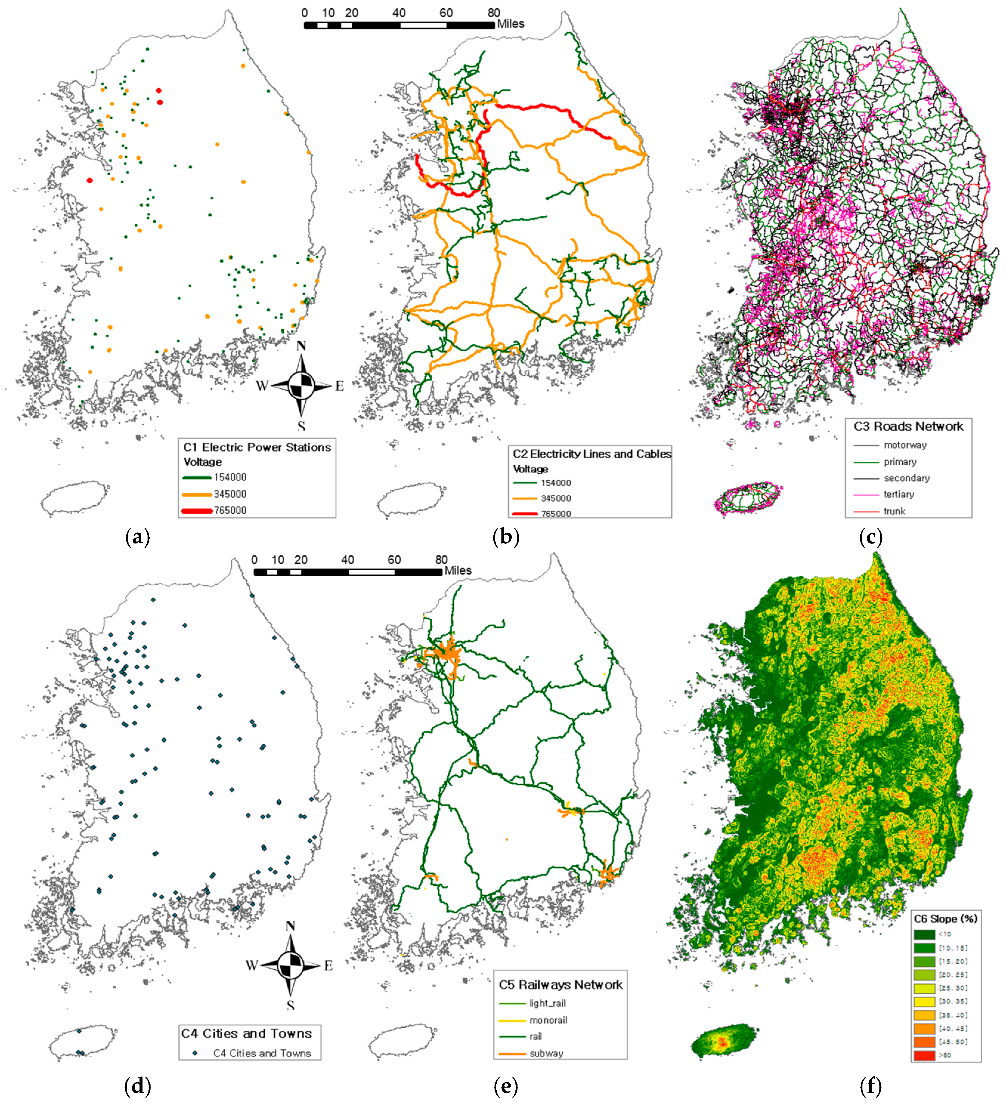
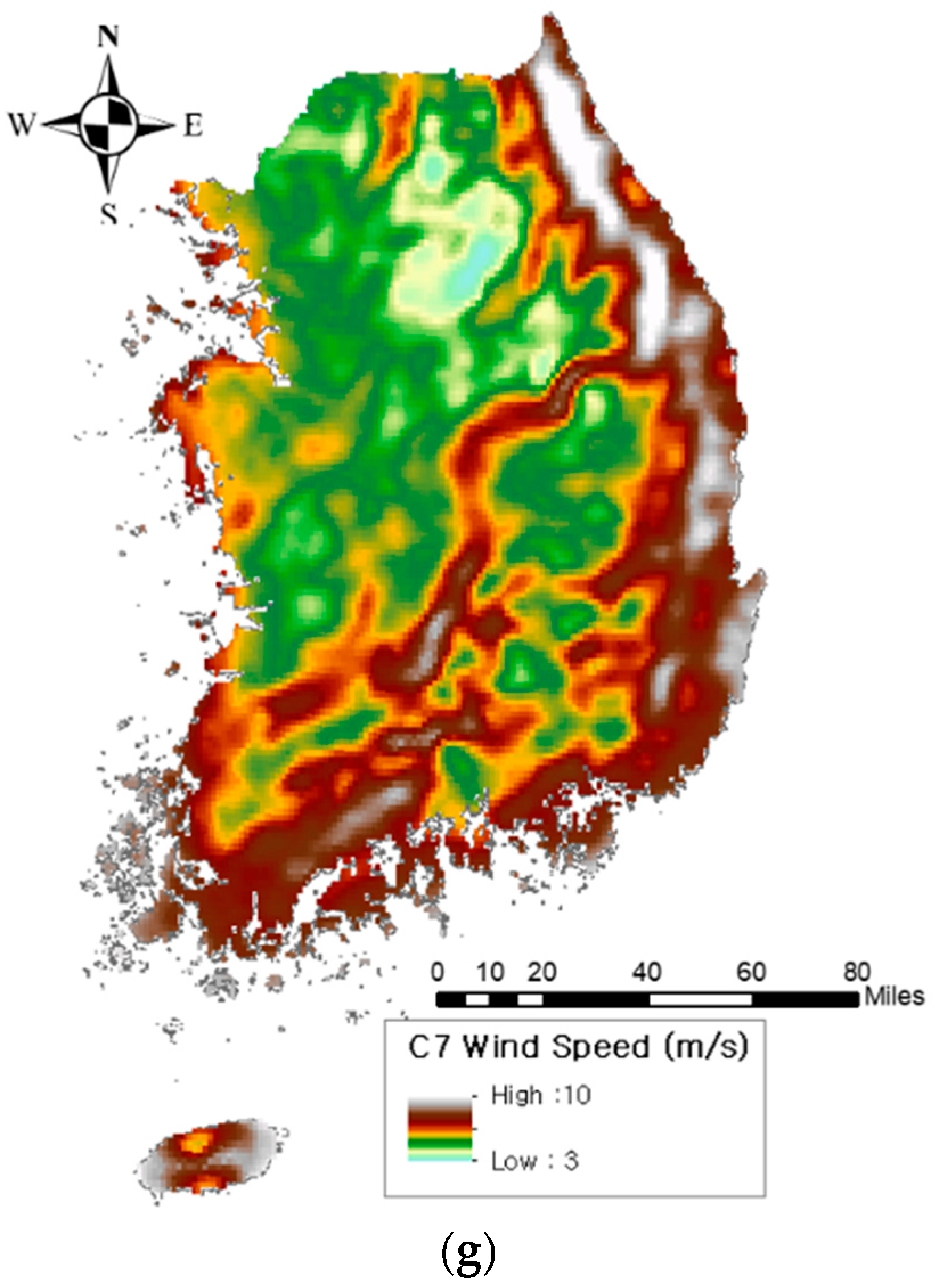
After the restricted areas were excluded from the total land of South Korea, the remainder is the land on which it is possible to erect an on-shore wind farm. The rest of the land must be evaluated on the basis of certain wind farm suitability criteria, and all such criteria used in the current study are shown in Figure 3.
It should be mentioned that on-shore wind farm site selection is not only limited to the criteria used in the current study, but this number may increase or decrease depending on the certain requirements of decision makers. These criteria were entered as input layers into GIS software tool and the corresponding maps are presented in Figure 3.
Any environmental or administrative factor that can have any sort of impact on the development of a wind farm has already been taken into account in the previous step, i.e., restricted or protected areas. Therefore, at this stage we will only consider the factors that may influence the decision making process of selecting the most suitable wind farm sites.
3. Results and Discussion
3.1. Multiple Scenarios
Wind farm development is highly sensitive to the opinions of different stake-holders, i.e., public, governments, wind farm developers, and many others. The criteria mentioned above are representing only the technical and economic aspects of the decision, but other issues such as social acceptance, public opinion, areas of special protection for birds, etc., are not considered here and are out of the scope of this study.
In order to create accurate wind farm suitability maps, it is very important to assign the weight to each criterion in a systematic and comprehensive way. For this purpose five experts in the field of renewable energy and wind power were asked to fill the fuzzy pairwise comparison table for all criteria and their responses are shown in Table 3, Table 4, Table 5, Table 6 and Table 7.
Equation (7) shows the calculations used to estimate the fuzzy geometric mean of criteria 1 expert 1:
Similarly, by using Equation (7) fuzzy geometric means for all the criteria were estimated in the case of expert 1 and are listed in Table 8.
In the next step, the fuzzy weight of criterion 1 in the case of expert 1 was estimated using following equation:
Hence the relative fuzzy weights, including lower and upper limits, of each criterion in the case of expert 1 are listed in Table 9.
In the final step, the fuzzy weights are converted into relative non-fuzzy weights (A) by taking the average of fuzzy numbers (l, m and u in Table 9) for each criterion. Then, by using non-fuzzy weights i.e., A’s values, the normalized weight w of each criterion is calculated and tabulated in Table 10.
If the same procedure is repeated for the rest of the tables i.e., Table 4, Table 5, Table 6 and Table 7, then the values of w of each criterion for all the experts can be easily calculated and are listed in Table 11. This can generate five different scenarios (Scenario 2 to 6) of developing on-shore wind farm suitability maps. One more case can also be created as well, by assigning the equal weights to each criterion (Scenario 1). So, we will consider a total of six different scenarios in this study with scenario 1 as an equal weights case, and scenario 2 (expert 1) to scenario 6 (expert 5).
Figure 4 show the relative distribution of each criterion’s fuzzy weights as function of fuzzy membership function as defined in Equation (1). C6 (slope) and C7 (wind speed) are two of the most important parameters that must be considered while designing the on-shore wind farm, as it is also clear from Figure 4 as well.
3.2. Wind Farm Suitability Maps
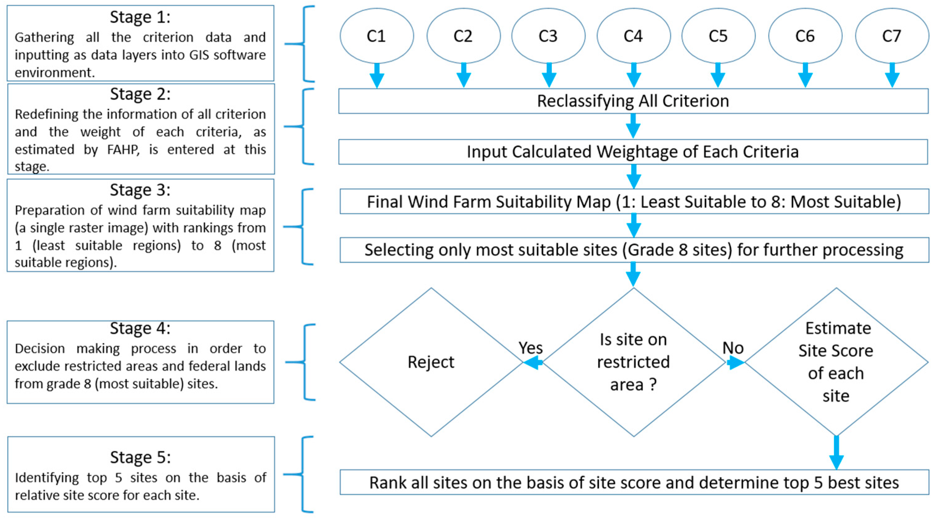
In order to start the analysis, the Euclidian distance of each cell in the map from the corresponding features in the criteria C1 to C5, was estimated. Euclidean distance, or Euclidean metric, is the “ordinary” straight-line distance between two points in Euclidean space. This was done in order to assign a rating to each part of the map of South Korea, i.e., parts of the country which are relatively nearer to the corresponding features in the afore mentioned five criteria, will get a higher rating than rest of the areas. Similarly, for C6 (slope), the flattest terrain got the highest ratings. On the other hand, for C7 (wind speed), locations with the maximum wind speed got the highest ratings and vice versa for other parts of the map. These modified seven criteria were then entered into the GIS software tool where they were re-classified (Stage 2 in Figure 5) as mentioned in above section. Figure 5 shows the overall procedure for developing on-shore wind farm suitability maps and the identification of top five most suitable sites.
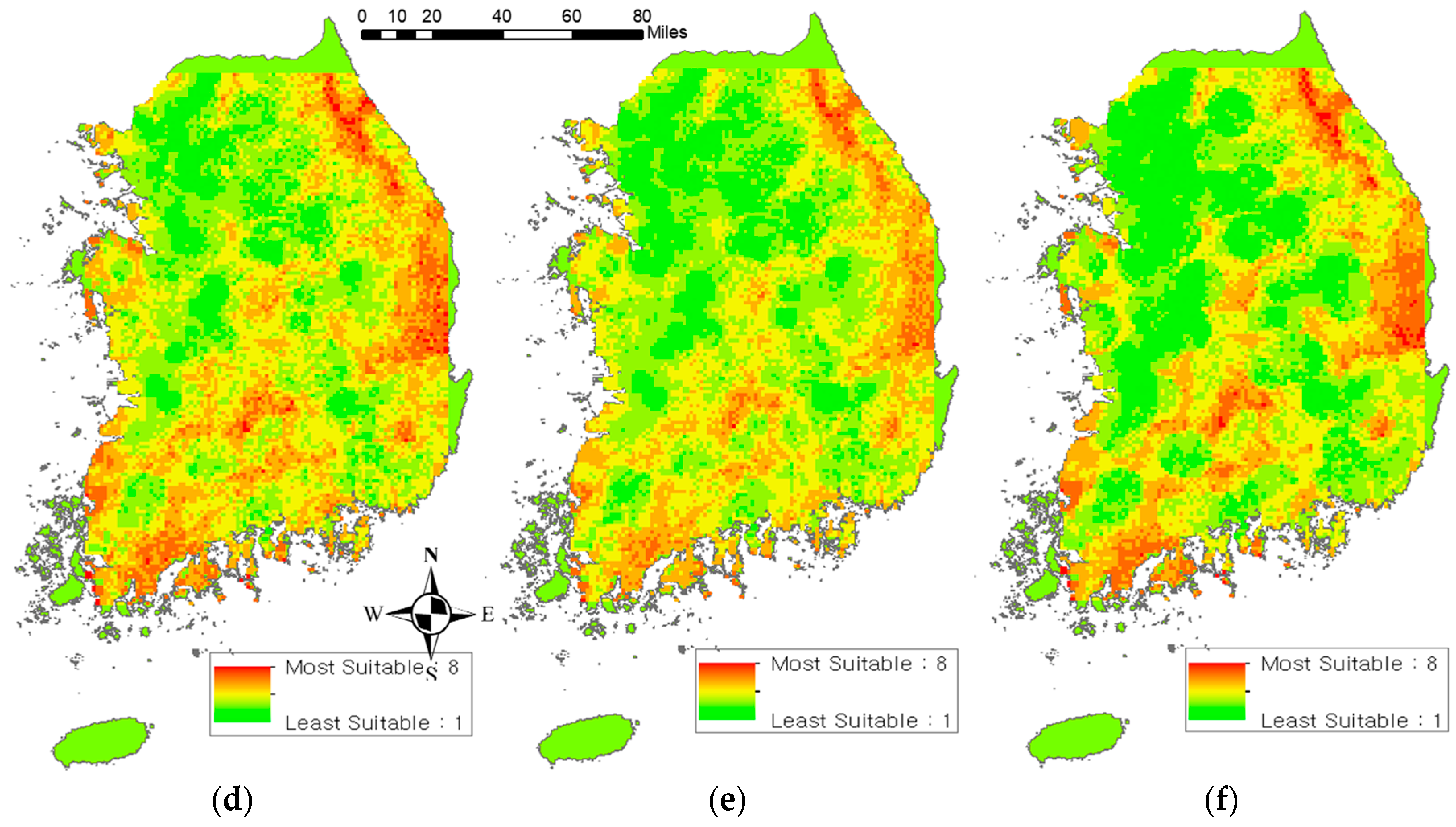
Using the thematic layers of the criteria and GIS software commands, such as Euclidean distance, slope, spatial analysis, area, intersection, erase, and buffers, it was possible to obtain the global thematic raster layers of on-shore wind farm suitability map, as shown in Figure 6. The suitability maps have been prepared for each of the six scenarios, and each location was scaled from 1 to 8; with 1 being the least suitable sites and 8 being the most suitable sites for on-shore wind farm development. From all the maps in Figure 6, it is clear that generally the eastern and the southwestern parts of the country are the most suitable areas for on-shore wind farm development.
The maps in Figure 6 can give an overall idea about the land distribution according to each scale, but it would be more useful if the exact areas of land can be estimated against each scale. Similar estimations have been made in Figure 7, which show the percentages of total land area of South Korea according to each scale. Figure 7 show that generally most of the land of South Korea is rated from 3–6 on the suitability scale, whereas out of all the six scenarios, the maximum percentage of sites rated an 8 is 0.68 (scenario 4) which corresponds to approximately 680 km2 of land.
3.3. Identification of Top Wind Farm Sites
This section deals with the identification, analysis and graphical representation of the suitability map’s sites scaled as 8 and also the top five the most optimal locations for on-shore wind farm development. Figure 8 show the exact locations of all 8 rated sites on the map of South Korea. Again, the same trend was found, that most suitable on-shore wind farm locations are situated either on the eastern side or southwestern side of the country. It should be noted that wind farm suitability maps presented in Figure 6 are covering the entirety of the land of the country, i.e., restricted areas as well, whereas on the other hand, restricted areas were excluded while preparing Figure 8 and Table 12, which lists the total area and number of sites available according to the sites rated as an 8 on the suitability maps.
As listed in Table 12, the total number of sites rated as an 8 are different according to each scenario. It would be more useful to identify the five best sites out of these rated 8 sites. For this purpose, the following Equation (9) was developed, which will assign a “site score” to each sites according to the average values of all seven criteria. The main idea of Equation (9) is that it will assign relatively higher site score to sites which have small values of criteria 1–6, i.e., minimum distance between a site and city, roads, etc., and has minimum slope. Whereas second part of Equation (9) indicates that sites having higher values of mean wind speed will get higher site score:
where Ci,j is the average value of ith criteria for jth site, Ci,min is the minimum value of ith criteria across all the scale 8 sites of a scenario, wi is the non-fuzzy normalized weigh of ith criteria (Table 11) and n is total number of suitability 8 rated sites in a particular scenario.
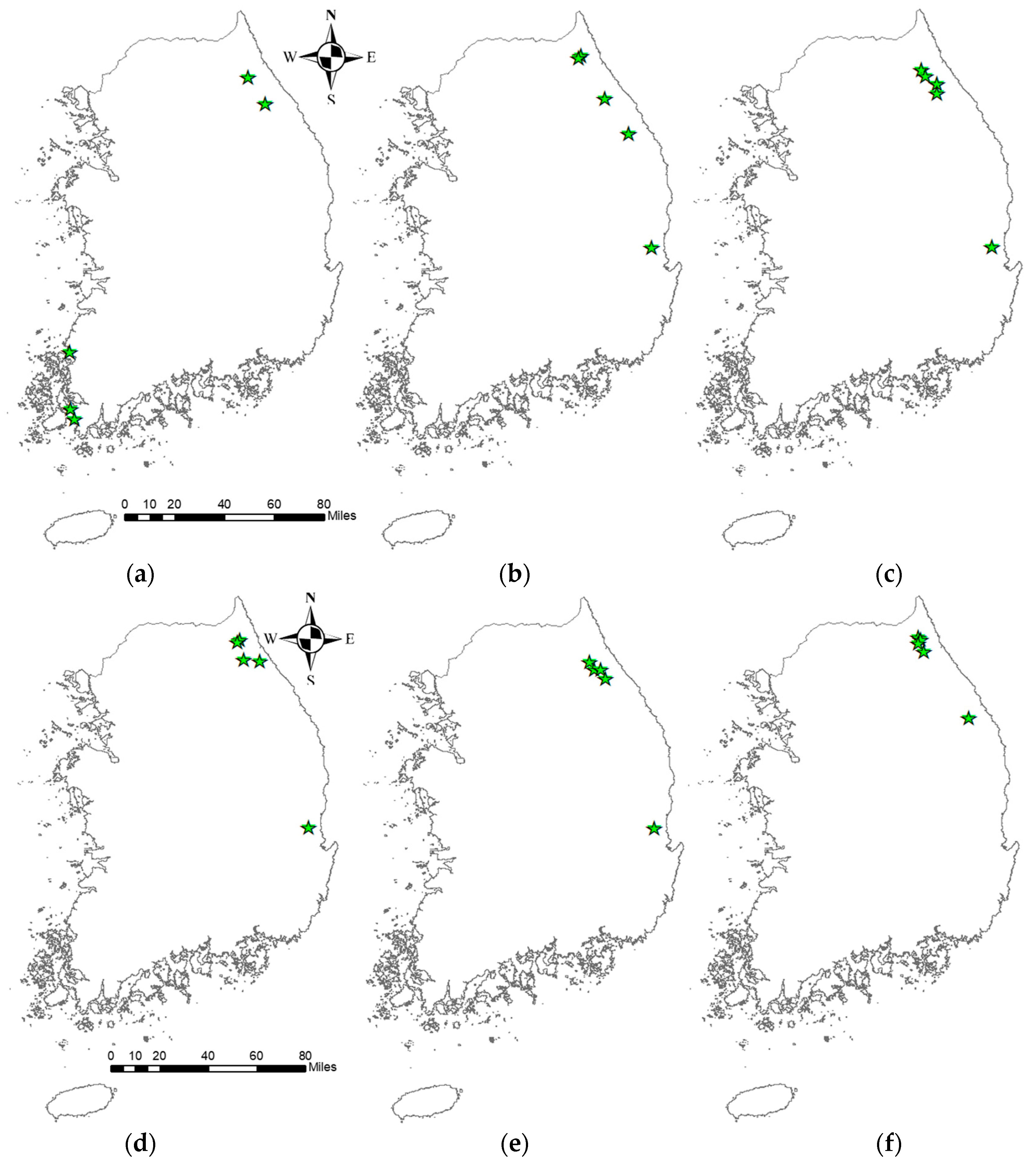
After estimating the site scores using Equation (9), Figure 9 and Table 13, Table 14, Table 15, Table 16, Table 17 and Table 18 were prepared on the basis of site score rankings. Figure 9 help to visualize the approximate locations of the top five most suitable on-shore wind farm sites according to all scenarios considered in this study. Whereas Table 13, Table 14, Table 15, Table 16, Table 17 and Table 18 include the exact locations, area availability, and average values of all seven criteria for each of the top five sites.
It should be explained that sites in Table 13, Table 14, Table 15, Table 16, Table 17 and Table 18 are being ranked on the basis of site score, calculated by using Equation (9), not on the basis of highest wind speeds. It can be observed in Table 13, Table 14, Table 15, Table 16, Table 17 and Table 18 that the sites with the highest site scores do not necessarily have the highest wind speeds. For instance, in Table 18, the site which is being placed at position 3, has the highest value of mean wind speed as compared to rest of the sites in same table, but at the same time the land slope is also the highest at this site. So the definition of “top site” really depends upon the technical preferences of the wind farm developers and designers. But if the top site is to be selected on the basis of MCDM, then it can be assumed that Equation (9) is a useful tool to identify the best suited wind farm locations as long as the weight assigned to each criterion is estimated carefully and correctly.
4. Conclusions
The current study deals with locating the most optimal on-shore wind farm locations in the territory of South Korea, using a comprehensive and structured GIS-MCDM approach. Selecting the optimal on-shore wind farm site is a quite complicated and multi-criteria decision process, as it engages and involves numerous stake-holders.
First of all, restricted areas such as military zones, federally protected areas, wetlands, etc., were excluded from the study zone. Then the remaining areas were evaluated on the basis of seven criteria, including wind speed, land slope and the distance from roads, which were assigned relative weights using the fuzzy-analytical hierarchy process (FAHP). Six scenarios were considered in this study and wind farm suitability maps (scaled from 1 to 8: with 1 being the least suitable site and vice versa for 8) were constructed for all the scenarios. It was found that eastern part of the country has the highest potential for hosting future on-shore wind farms, whereas northwestern areas are the least suitable region for this purpose. The total area of the sites rated as an 8 for each scenario was almost less than 0.7 percent of the total land area of South Korea, which corresponds to approximately 700 km2 of land. In order to visualize the exact locations of sites that were rated as an 8, excluding the restricted areas, all the sites are being depicted on maps as well. Finally, out of these sites, the top five best sites were determined according to the weights assigned to each criterion using the FAHP methodology. The important parameters such as latitude (°), longitude (°), area available (km2), and average values of each of the seven criteria were estimated for each of the top five most suitable sites. The site location (latitude: 34.58° and longitude: 138.42°) was found to be the overall most suitable location for developing an on-shore wind farm, having total area of 29.4 km2 and the mean wind speed 50 m above ground-level was found to be 6.61 m/s.
Acknowledgments
This work was supported by the new and renewable energy core technology program of the Korean Institute of Energy Technology Evaluation and Planning (KETEP), granted financial resources from the Ministry of Trade, Industry and Energy, Republic of Korea (No. 20153010130310).
Author Contributions
Sajid Ali and Sang-Moon Lee collected the GIS data whereas Choon-Man Jang provided his technical support throughout the study. Sajid Ali analyzed the data and wrote the paper.
Conflicts of Interest
The authors declare no conflict of interest.
Nomenclature
| i | i-th value of a parameter |
| Fuzzy triangular membership function | |
| w | Non-fuzzy normalized weightage assigned to each criteria |
| l | Lower limit of criteria weightage |
| m | Mean value of criteria weightage |
| u | Upper limit of criteria weightage |
| n | Number of criteria |
| C | Criteria |
| E | Expert |
| R | Restricted areas |
| Fuzzy matrix | |
| Cij | Relative score of i-th criteria w.r.t. j-th criteria |
| Ci,j | Average value of i-th criteria for j-th site |
| Geometric mean of fuzzy numbers assigned to a criteria | |
| A | Non-normalized non-fuzzy weight of a criteria (de-fuzzification) |
| Ci,min | The minimum value of i-th criteria across all sites |
| Ci,max | The maximum value of i-th criteria across all sites |
References
- Van Haaren, R.; Fthenakis, V. GIS-based wind farm site selection using spatial multi-criteria analysis (SMCA): Evaluating the case for New York State. Renew. Sustain. Energy Rev. 2011, 15, 3332–3340. [Google Scholar] [CrossRef]
- Latinopoulos, D.; Kechagia, K. A GIS-based multi-criteria evaluation for wind farm site selection. A regional scale application in Greece. Renew. Energy 2015, 78, 550–560. [Google Scholar] [CrossRef]
- Noorollahi, Y.; Yousefi, H.; Mohammadi, M. Multi-criteria decision support system for wind farm site selection using GIS. Sustain. Energy Technol. Assess. 2016, 13, 38–50. [Google Scholar]
- Janke, J.R. Multi-criteria GIS modeling of wind and solar farms in Colorado. Renew. Energy 2010, 35, 2228–2234. [Google Scholar] [CrossRef]
- Rodman, L.C.; Meentemeyer, R.K. A geographic analysis of wind turbine placement in Northern California. Energy Policy 2006, 34, 2137–2149. [Google Scholar] [CrossRef]
- Grassi, S.; Chokani, N.; Abhari, R.S. Large scale technical and economical assessment of wind energy potential with a GIS tool: Case study Iowa. Energy Policy 2012, 45, 73–85. [Google Scholar] [CrossRef]
- Yue, C.-D.; Wang, S.-S. GIS-based evaluation of multifarious local renewable energy sources: A case study of the Chigu area of southwestern Taiwan. Energy Policy 2006, 34, 730–742. [Google Scholar] [CrossRef]
- Baban, S.M.; Parry, T. Developing and applying a GIS-assisted approach to locating wind farms in the UK. Renew. Energy 2001, 24, 59–71. [Google Scholar] [CrossRef]
- Park, U.-S.; Yoo, N.-S.; Kim, J.-H.; Kim, K.-S.; Min, D.-H.; Lee, S.-W.; Kim, H.-G. The Selection of Promising Wind Farm Sites in Gangwon Province using Multi Exclusion Analysis. J. Korean Solar Energy Soc. 2015, 35, 1–10. [Google Scholar] [CrossRef]
- Kim, H.-G. Preliminary estimation of wind resource potential in South Korea. J. Korean Solar Energy Soc. 2008, 28, 1–7. [Google Scholar]
- Jang, J.-K.; Yu, B.-M.; Ryu, K.-W.; Lee, J.-S. Offshore wind resource assessment around Korean Peninsula by using QuikSCAT satellite data. J. Korean Soc. Aeronaut. Space Sci. 2009, 37, 1121–1130. [Google Scholar] [CrossRef]
- Oh, K.-Y.; Kim, J.-Y.; Lee, J.-K.; Ryu, M.-S.; Lee, J.-S. An assessment of wind energy potential at the demonstration offshore wind farm in Korea. Energy 2012, 46, 555–563. [Google Scholar] [CrossRef]
- Kim, H.; Kim, B. Wind resource assessment and comparative economic analysis using AMOS data on a 30 MW wind farm at Yulchon district in Korea. Renew. Energy 2016, 85, 96–103. [Google Scholar] [CrossRef]
- Lee, M.E.; Kim, G.; Jeong, S.-T.; Ko, D.H.; Kang, K.S. Assessment of offshore wind energy at Younggwang in Korea. Renew. Sustain. Energy Rev. 2013, 21, 131–141. [Google Scholar] [CrossRef]
- Kim, J.-Y.; Oh, K.-Y.; Kang, K.-S.; Lee, J.-S. Site selection of offshore wind farms around the Korean Peninsula through economic evaluation. Renew. Energy 2013, 54, 189–195. [Google Scholar] [CrossRef]
- Oh, K.-Y.; Kim, J.-Y.; Lee, J.-S.; Ryu, K.-W. Wind resource assessment around Korean Peninsula for feasibility study on 100 MW class offshore wind farm. Renew. Energy 2012, 42, 217–226. [Google Scholar] [CrossRef]
- Saaty, T.L. The Analytic Hierarchy Process; McGraw Hill International: New York City, NY, USA, 1980. [Google Scholar]
- Zadeh, L.A. “Fuzzy Sets”. Inf. Control 1965, 8, 199–249. [Google Scholar] [CrossRef]
- Ruoning, X.; Xiaoyan, Z. Extensions of the analytic hierarchy process in fuzzy environment. Fuzzy Sets Syst. 1992, 52, 251–257. [Google Scholar] [CrossRef]
- Cheng, C.-H.; Yang, K.-L.; Hwang, C.-L. Evaluating attack helicopters by AHP based on linguistic variable weight. Eur. J. Oper. Res. 1999, 116, 423–435. [Google Scholar] [CrossRef]
- Cheng, C.-H. Evaluating naval tactical missile systems by fuzzy AHP based on the grade value of membership function. Eur. J. Oper. Res. 1997, 96, 343–350. [Google Scholar] [CrossRef]
- Petkovic, J.; Sevarac, Z.; Jaksic, M.L.; Marinkovic, S. Application of fuzzy AHP method for choosing a technology within Service Company. Tech. Technol. Educ. Manag. TTEM 2012, 7, 332–341. [Google Scholar]
- Bellman, R.E.; Zadeh, L.A. Decision-making in a fuzzy environment. Manag. Sci. 1970, 17, B-141–B-164. [Google Scholar] [CrossRef]
- Garcia-Cascales, M.S.; Lamata, M.T. Multi-criteria analysis for a maintenance management problem in an engine factory: Rational choice. J. Intell. Manuf. 2011, 22, 779–788. [Google Scholar] [CrossRef]
- Klir, G.; Yuan, B. Fuzzy Sets and Fuzzy Logic: Theory and Applications; Prentice Hall: Upper Saddle River, NJ, USA, 1995; Volume 4. [Google Scholar]
- Kilincci, O.; Onal, S.A. Fuzzy AHP approach for supplier selection in a washing machine company. Expert Syst. Appl. 2011, 38, 9656–9664. [Google Scholar] [CrossRef]
- Van Laarhoven, P.; Pedrycz, W. A fuzzy extension of Saaty’s priority theory. Fuzzy Sets Syst. 1983, 11, 229–241. [Google Scholar] [CrossRef]
- Chang, D.-Y. Applications of the extent analysis method on fuzzy AHP. Eur. J. Oper. Res. 1996, 95, 649–655. [Google Scholar] [CrossRef]
- Jaber, J.; Jaber, Q.; Sawalha, S.; Mohsen, M. Evaluation of conventional and renewable energy sources for space heating in the household sector. Renew. Sustain. Energy Rev. 2008, 12, 278–289. [Google Scholar] [CrossRef]
- Kahraman, C.; Kaya, İ.; Cebi, S. A comparative analysis for multi attribute selection among renewable energy alternatives using fuzzy axiomatic design and fuzzy analytic hierarchy process. Energy 2009, 34, 1603–1616. [Google Scholar] [CrossRef]
- Heo, E.; Kim, J.; Boo, K.-J. Analysis of the assessment factors for renewable energy dissemination program evaluation using fuzzy AHP. Renew. Sustain. Energy Rev. 2010, 14, 2214–2220. [Google Scholar] [CrossRef]
- Tasri, A.; Susilawati, A. Selection among renewable energy alternatives based on a fuzzy analytic hierarchy process in Indonesia. Sustain. Energy Technol. Assess. 2014, 7, 34–44. [Google Scholar] [CrossRef]
- Ren, J.; Sovacool, B.K. Enhancing China’s energy security: Determining influential factors and effective strategic measures. Energy Convers. Manag. 2014, 88, 589–597. [Google Scholar] [CrossRef]
- Chang, N.-B.; Chang, Y.-H.; Chen, H.-W. Fair fund distribution for a municipal incinerator using GIS-based fuzzy analytic hierarchy process. J. Environ. Manag. 2009, 90, 441–454. [Google Scholar] [CrossRef] [PubMed]
- Chen, H.H.; Kang, H.-Y.; Lee, A.H. Strategic selection of suitable projects for hybrid solar-wind power generation systems. Renew. Sustain. Energy Rev. 2010, 14, 413–421. [Google Scholar] [CrossRef]
- Lee, A.H.; Chen, H.H.; Kang, H.-Y. A model to analyze strategic products for photovoltaic silicon thin-film solar cell power industry. Renew. Sustain. Energy Rev. 2011, 15, 1271–1283. [Google Scholar] [CrossRef]
- Yeh, T.-M.; Huang, Y.-L. Factors in determining wind farm location: Integrating GQM, fuzzy DEMATEL, and ANP. Renew. Energy 2014, 66, 159–169. [Google Scholar] [CrossRef]
- Shafiee, M. A fuzzy analytic network process model to mitigate the risks associated with offshore wind farms. Expert Syst. Appl. 2015, 42, 2143–2152. [Google Scholar] [CrossRef]
- Liu, S.; Zhang, J.; Liu, W.; Qian, Y. A comprehensive decision-making method for wind power integration projects based on improved fuzzy AHP. Energy Procedia 2012, 14, 937–942. [Google Scholar] [CrossRef]
- Lee, A.H.; Hung, M.-C.; Kang, H.-Y.; Pearn, W. A wind turbine evaluation model under a multi-criteria decision making environment. Energy Convers. Manag. 2012, 64, 289–300. [Google Scholar] [CrossRef]
- Buckley, J.J. Fuzzy hierarchical analysis. Fuzzy Sets Syst. 1985, 17, 233–247. [Google Scholar] [CrossRef]
- Chou, S.-W.; Chang, Y.-C. The implementation factors that influence the ERP (enterprise resource planning) benefits. Decis. Support Syst. 2008, 46, 149–157. [Google Scholar] [CrossRef]
- Stat Silk. Available online: https://www.statsilk.com (accessed on 20 September 2017).
- Geofabrik Downloads. Available online: http://download.geofabrik.de/asia/south-korea.html (accessed on 20 September 2017).
- Osm2Shp. Available online: http://osm2shp.ru/ (accessed on 20 September 2017).
- Global Administrative Areas. Available online: http://www.gadm.org/country (accessed on 20 September 2017).
- DIVA-GIS. Available online: http://www.diva-gis.org/gdata (accessed on 20 September 2017).
- Open Street Map Data, Ruduced Waterbodies as Polygons. Available online: http://openstreetmapdata.com/data/water-reduced-polygons (accessed on 20 September 2017).
- MapCruzin. Available online: http://www.mapcruzin.com (accessed on 20 September 2017).
- USGS Science for a Changing World. Available online: https://landcover.usgs.gov/globallandcover.php# (accessed on 20 September 2017).
Figure 1.
A typical fuzzy triangular number and its weight.
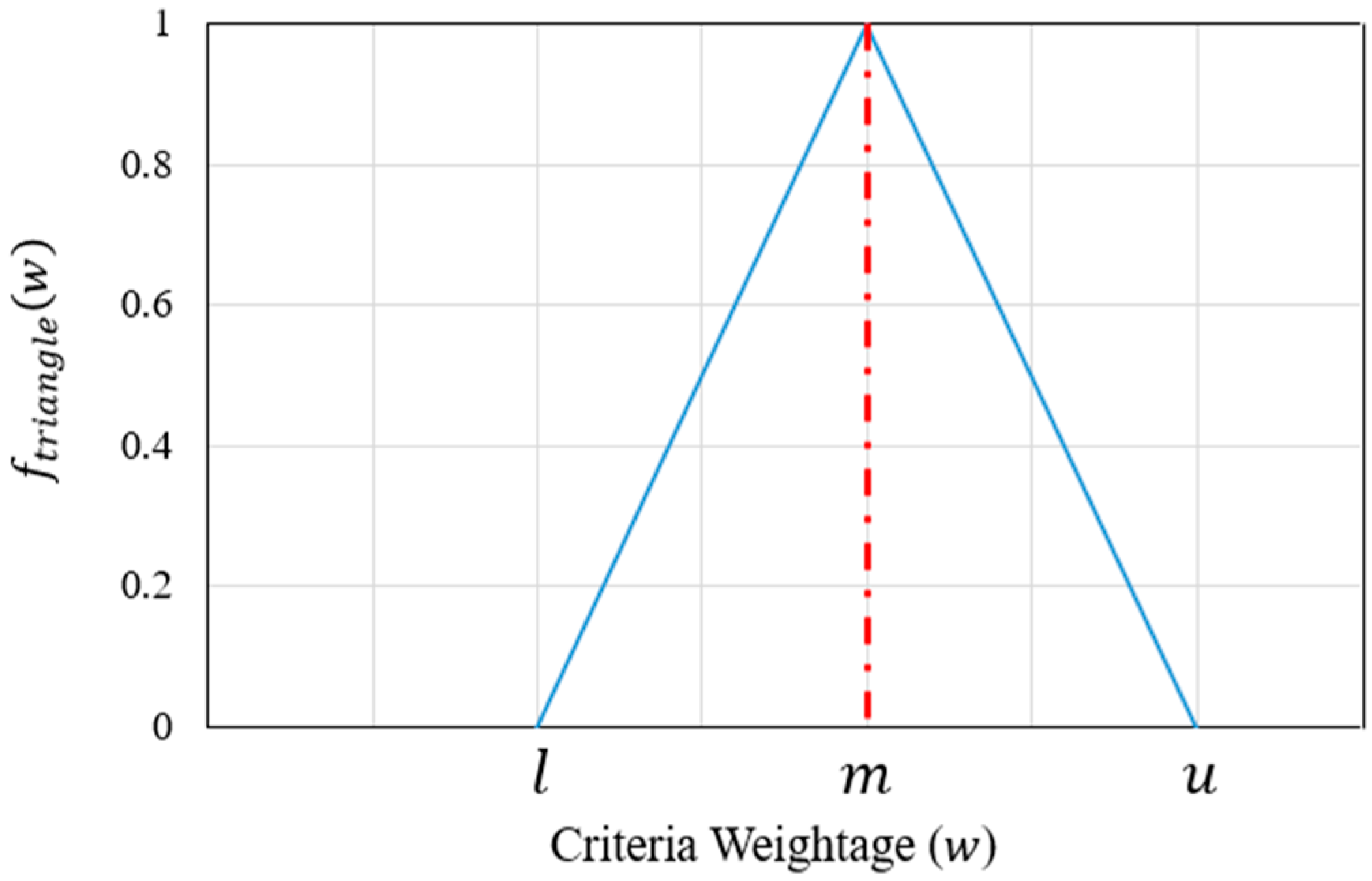
Figure 2.
Restricted areas for wind farm development (a) R1: Military Zones and Protected Areas (b) R2: Land Under Use (c) R3: Tourism, Historic, Cultural and Religious Places (d) R4: Natural and Federal Areas (e) R5: Railways and Subways Network (f) R6: Wetlands, Rivers, Lakes, Water reservoirs and Streams (g) R7: Public and Community Interest Places.
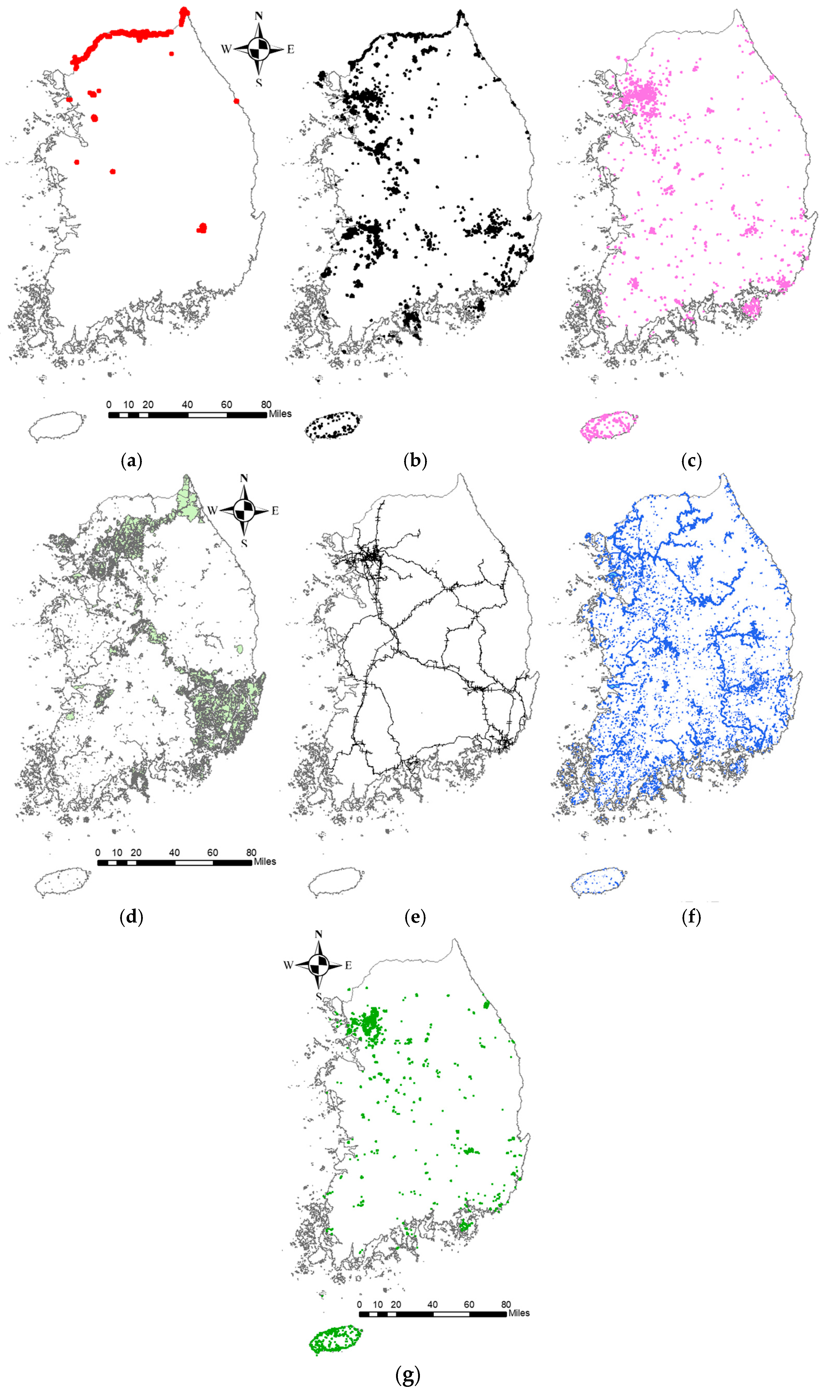
Figure 3.
Criterion (a) C1: Electric Power Stations (b) C2: Electricity Lines and Cables (c) C3: Roads Network (d) C4: Cities and Towns with population greater than 10 k (e) C5: Railways Network (f) C6: Land Slope (%) (g) C7: Wind Speed (m/s).
Figure 3.
Criterion (a) C1: Electric Power Stations (b) C2: Electricity Lines and Cables (c) C3: Roads Network (d) C4: Cities and Towns with population greater than 10 k (e) C5: Railways Network (f) C6: Land Slope (%) (g) C7: Wind Speed (m/s).


Figure 4.
Fuzzy triangular weights for each criteria according to each expert (a) Expert 1 (b) Expert 2 (c) Expert 3 (d) Expert 4 (e) Expert 5.
Figure 4.
Fuzzy triangular weights for each criteria according to each expert (a) Expert 1 (b) Expert 2 (c) Expert 3 (d) Expert 4 (e) Expert 5.
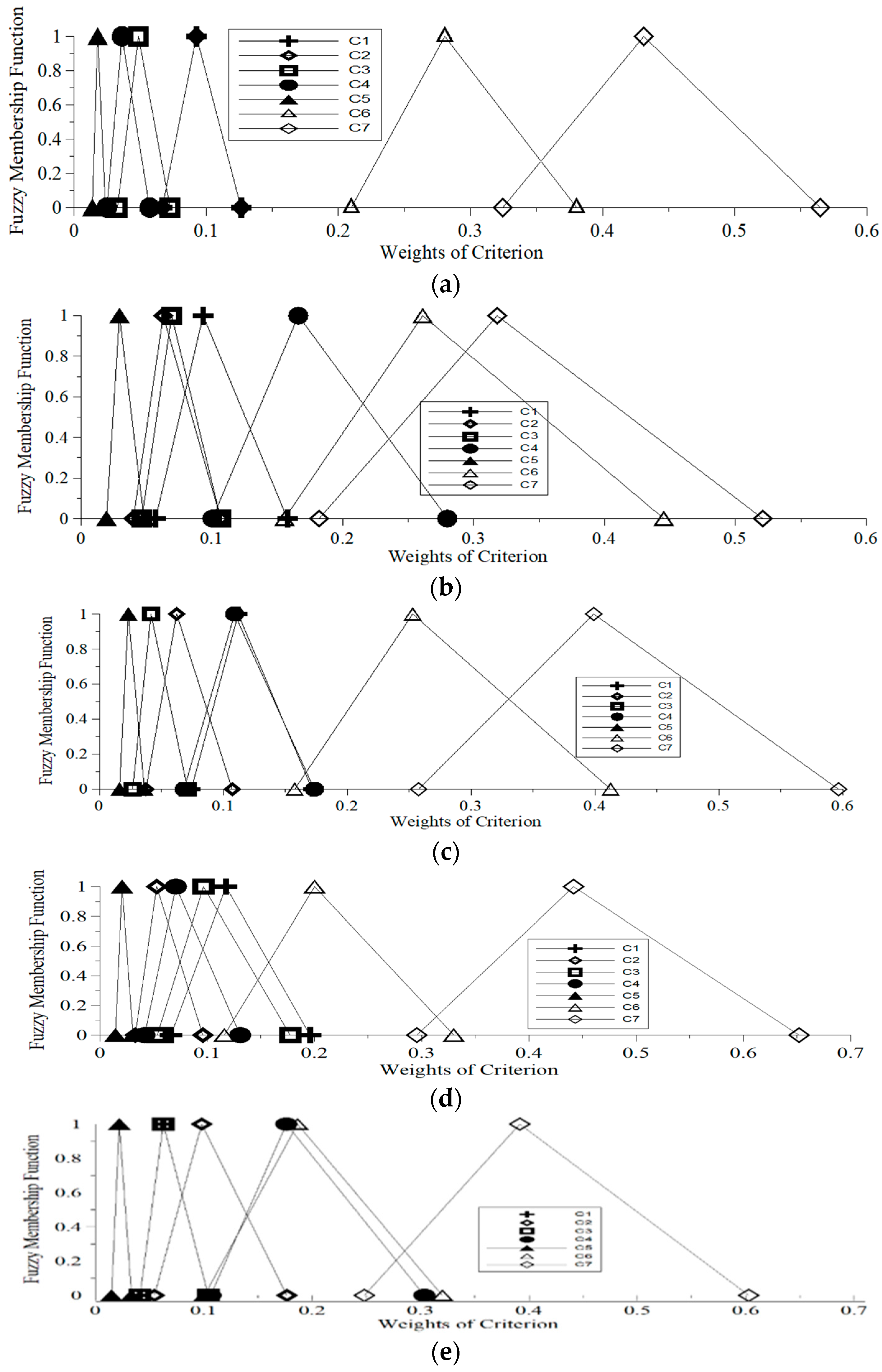
Figure 5.
Layout process for development of wind farm suitability maps.

Figure 6.
Wind farm suitability maps (a) Scenario 1 (b) Scenario 2 (c) Scenario 3 (d) Scenario 4 (e) Scenario 5 (f) Scenario 6.
Figure 6.
Wind farm suitability maps (a) Scenario 1 (b) Scenario 2 (c) Scenario 3 (d) Scenario 4 (e) Scenario 5 (f) Scenario 6.
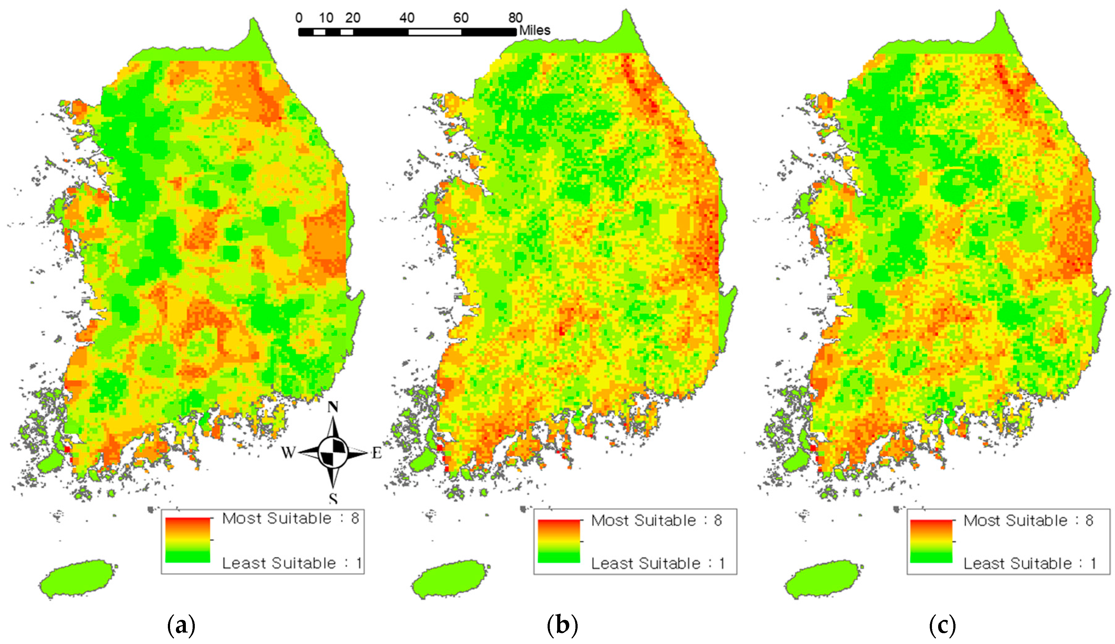

Figure 7.
Divisions of South Korean land territory according to different wind farm suitability scales (a) Scenario 1 (b) Scenario 2 (c) Scenario 3 (d) Scenario 4 (e) Scenario 5 (f) Scenario 6.
Figure 7.
Divisions of South Korean land territory according to different wind farm suitability scales (a) Scenario 1 (b) Scenario 2 (c) Scenario 3 (d) Scenario 4 (e) Scenario 5 (f) Scenario 6.
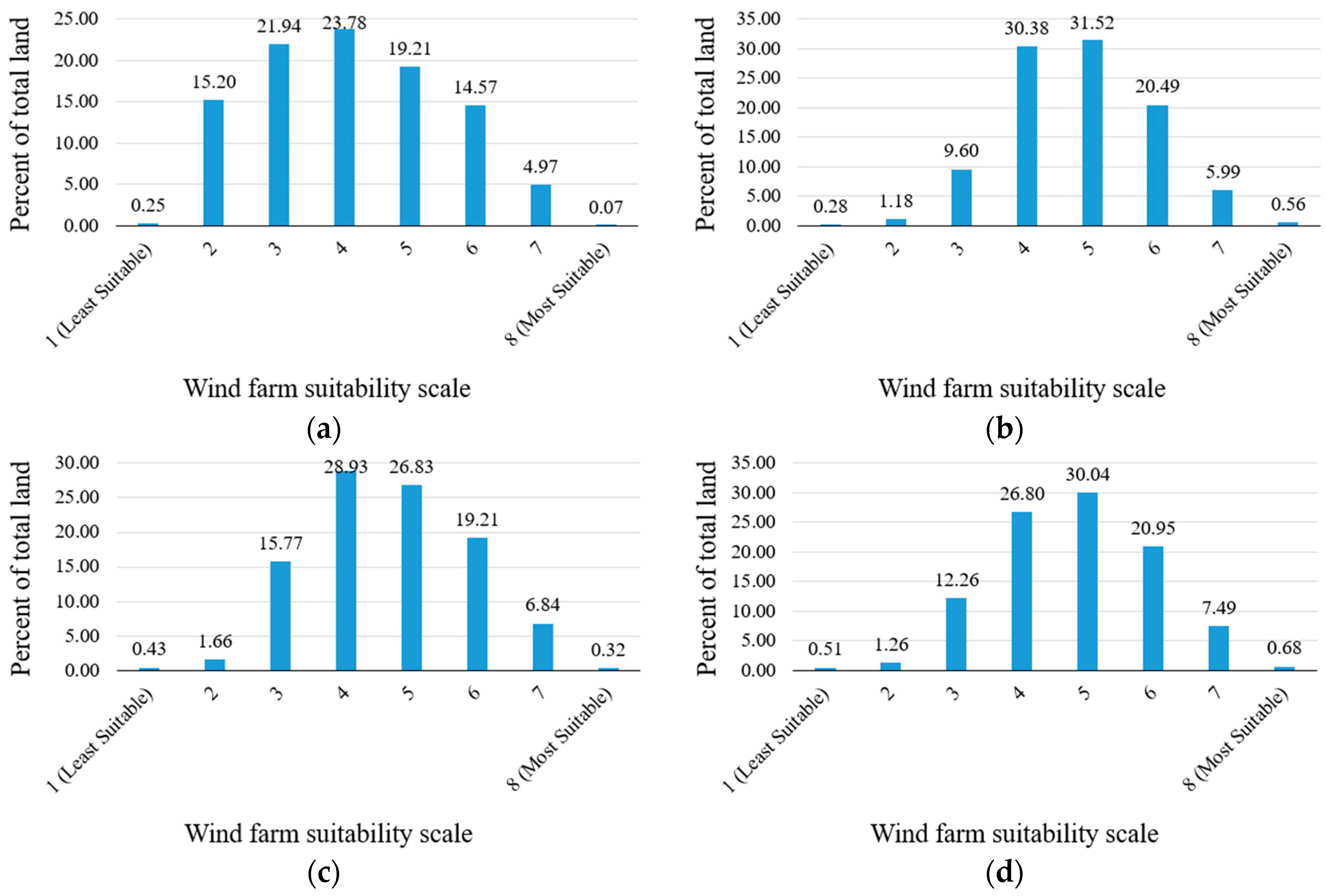
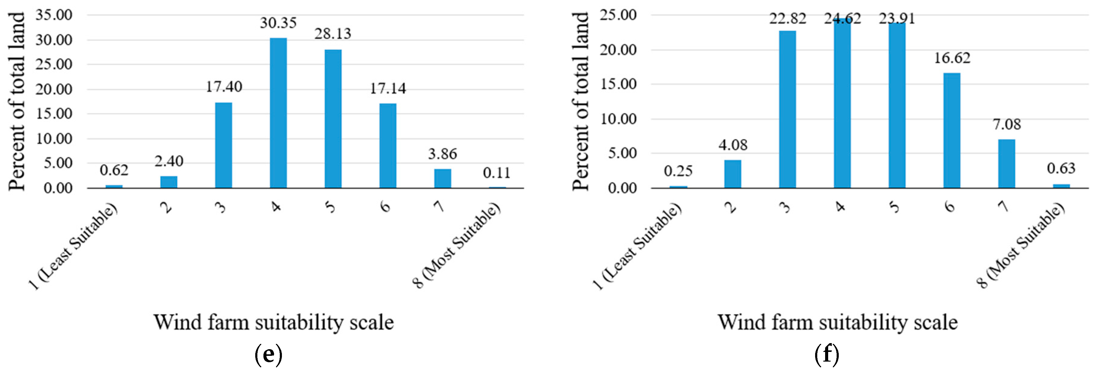
Figure 8.
Wind farm suitability scale 8 (most suitable) sites excluding restricted areas (a) Scenario 1 (b) Scenario 2 (c) Scenario 3 (d) Scenario 4 (e) Scenario 5 (f) Scenario 6.
Figure 8.
Wind farm suitability scale 8 (most suitable) sites excluding restricted areas (a) Scenario 1 (b) Scenario 2 (c) Scenario 3 (d) Scenario 4 (e) Scenario 5 (f) Scenario 6.
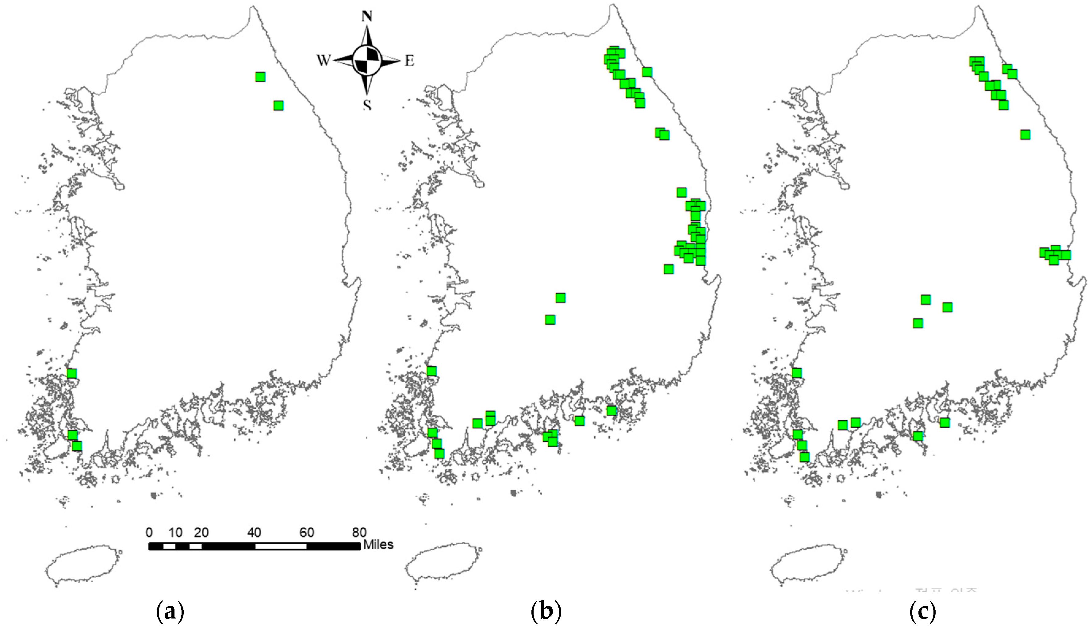
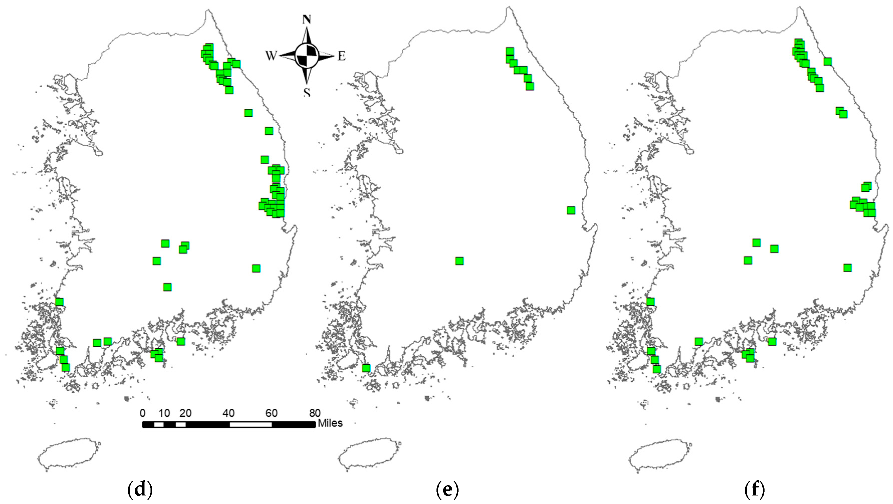
Figure 9.
Top 5 most suitable wind farm sites excluding restricted areas (a) Scenario 1 (b) Scenario 2 (c) Scenario 3 (d) Scenario 4 (e) Scenario 5 (f) Scenario 6.
Figure 9.
Top 5 most suitable wind farm sites excluding restricted areas (a) Scenario 1 (b) Scenario 2 (c) Scenario 3 (d) Scenario 4 (e) Scenario 5 (f) Scenario 6.

Table 1.
Definition of FAHP scale.
| AHP Scale | Linguistic Statement | FAHP Scale |
|---|---|---|
| 1 | Equally important | (1, 1, 1) |
| 3 | Weakly important | (2, 3, 4) |
| 5 | Fairly important | (4, 5, 6) |
| 7 | Strongly important | (6, 7, 8) |
| 9 | Absolutely important | (9, 9, 9 |
| 2 | Interpolation scale | (1, 2, 3) |
| 4 | (3, 4, 5) | |
| 6 | (5, 6, 7) | |
| 8 | (7, 8, 9) |
Table 2.
Applications of FAHP as MCDA technique in previous renewable energy studies.
| Field of Research | References |
|---|---|
| Space heating [29] | Jaber et al. [29] |
| Renewables [30,31,32,33] | Kahraman et al. [30] |
| Heo et al. [31] | |
| Tasri and Susilawati [32] | |
| Ren and Sovacool [33] | |
| Bio Energy [34] | Chang et al. [34] |
| Hybrid [35] | Chen et al. [35] |
| Solar [36] | Lee et al. [36] |
| Wind [37,38,39,40] | Yeh and Huang [37] |
| Shafiee [38] | |
| Liu et al. [39] | |
| Lee et al. [40] |
Table 3.
Fuzzy Comparisons for each criteria (Expert 1).
| Criteria | C1 | C2 | C3 | C4 | C5 | C6 | C7 |
|---|---|---|---|---|---|---|---|
| C1 | (1, 1, 1) | (1, 1, 1) | (2, 3, 4) | (2, 3, 4) | (6, 7, 8) | (1/6, 1/5, 1/4) | (1/8, 1/7, 1/6) |
| C2 | (1, 1, 1) | (1, 1, 1) | (2, 3, 4) | (2, 3, 4) | (6, 7, 8) | (1/6, 1/5, 1/4) | (1/8, 1/7, 1/6) |
| C3 | (1/4, 1/3, 1/2) | (1/4, 1/3, 1/2) | (1, 1, 1) | (1, 2, 3) | (4, 5, 6) | (1/8, 1/7, 1/6) | (1/9, 1/8, 1/7) |
| C4 | (1/4, 1/3, 1/2) | (1/4, 1/3, 1/2) | (1/3, 1/2, 1) | (1, 1, 1) | (2, 3, 4) | (1/9, 1/8, 1/7) | (1/9, 1/8, 1/7) |
| C5 | (1/8, 1/7, 1/6) | (1/8, 1/7, 1/6) | (1/6, 1/5, 1/4) | (1/4, 1/3, 1/2) | (1, 1, 1) | (1/9, 1/9, 1/9) | (1/9, 1/9, 1/9) |
| C6 | (4, 5, 6) | (4, 5, 6) | (6, 7, 8) | (7, 8, 9) | (9, 9, 9) | (1, 1, 1) | (1/4, 1/3, 1/2) |
| C7 | (6, 7, 8) | (6, 7, 8) | (7, 8, 9) | (7, 8, 9) | (9, 9, 9) | (2, 3, 4) | (1, 1, 1) |
Table 4.
Fuzzy Comparisons for each criteria (Expert 2).
| Criteria | C1 | C2 | C3 | C4 | C5 | C6 | C7 |
|---|---|---|---|---|---|---|---|
| C1 | (1, 1, 1) | (1, 2, 3) | (1, 1, 1) | (1/4, 1/3, 1/2) | (4, 5, 6) | (1/4, 1/3, 1/2) | (1/4, 1/3, 1/2) |
| C2 | (1/3, 1/2, 1) | (1, 1, 1) | (1, 1, 1) | (1/5, 1/4, 1/3) | (2, 3, 4) | (1/5, 1/4, 1/3) | (1/5, 1/4, 1/3) |
| C3 | (1, 1, 1) | (1, 1, 1) | (1, 1, 1) | (1/5, 1/4, 1/3) | (2, 3, 4) | (1/5, 1/4, 1/3) | (1/5, 1/4, 1/3) |
| C4 | (2, 3, 4) | (3, 4, 5) | (3, 4, 5) | (1, 1, 1) | (3, 4, 5) | (1/4, 1/3, 1/2) | (1/4, 1/3, 1/2) |
| C5 | (1/6, 1/5, 1/4) | (1/4, 1/3, 1/2) | (1/4, 1/3, 1/2) | (1/5, 1/4, 1/3) | (1, 1, 1) | (1/8, 1/7, 1/6) | (1/8, 1/7, 1/6) |
| C6 | (2, 3, 4) | (3, 4, 5) | (3, 4, 5) | (2, 3, 4) | (6, 7, 8) | (1, 1, 1) | (1/3, 1/2, 1) |
| C7 | (2, 3, 4) | (3, 4, 5) | (3, 4, 5) | (2, 3, 4) | (6, 7, 8) | (1, 2, 3) | (1, 1, 1) |
Table 5.
Fuzzy Comparisons for each criteria (Expert 3).
| Criteria | C1 | C2 | C3 | C4 | C5 | C6 | C7 |
|---|---|---|---|---|---|---|---|
| C1 | (1, 1, 1) | (2, 3, 4) | (2, 3, 4) | (1, 1, 1) | (5, 6, 7) | (1/4, 1/3, 1/2) | (1/7, 1/6, 1/5) |
| C2 | (1/4, 1/3, 1/2) | (1, 1, 1) | (1, 2, 3) | (1/3, 1/2, 1) | (3, 4, 5) | (1/5, 1/4, 1/3) | (1/8, 1/7, 1/6) |
| C3 | (1/4, 1/3, 1/2) | (1/3, 1/2, 1) | (1, 1, 1) | (1/4, 1/3, 1/2) | (2, 3, 4) | (1/8, 1/7, 1/6) | (1/9, 1/8, 1/7) |
| C4 | (1, 1, 1) | (1, 2, 3) | (2, 3, 4) | (1, 1, 1) | (4, 5, 6) | (1/4, 1/3, 1/2) | (1/5, 1/4, 1/3) |
| C5 | (1/7, 1/6, 1/5) | (1/5, 1/4, 1/3) | (1/4, 1/3, 1/2) | (1/6, 1/5, 1/4) | (1, 1, 1) | (1/8, 1/7, 1/6) | (1/9, 1/8, 1/7) |
| C6 | (2, 3, 4) | (3, 4, 5) | (6, 7, 8) | (2, 3, 4) | (6, 7, 8) | (1, 1, 1) | (1/3, 1/2, 1) |
| C7 | (5, 6, 7) | (6, 7, 8) | (7, 8, 9) | (3, 4, 5) | (7, 8, 9) | (1, 2, 3) | (1, 1, 1) |
Table 6.
Fuzzy Comparisons for each criteria (Expert 4).
| Criteria | C1 | C2 | C3 | C4 | C5 | C6 | C7 |
|---|---|---|---|---|---|---|---|
| C1 | (1, 1, 1) | (2, 3, 4) | (1, 2, 3) | (1, 2, 3) | (5, 6, 7) | (1/4, 1/3, 1/2) | (1/7, 1/6, 1/5) |
| C2 | (1/4, 1/3, 1/2) | (1, 1, 1) | (1/3, 1/2, 1) | (1/3, 1/2, 1) | (4, 5, 6) | (1/5, 1/4, 1/3) | (1/8, 1/7, 1/6) |
| C3 | (1/3, 1/2, 1) | (1, 2, 3) | (1, 1, 1) | (1, 2, 3) | (5, 6, 7) | (1/3, 1/2, 1) | (1/7, 1/6, 1/5) |
| C4 | (1/3, 1/2, 1) | (1, 2, 3) | (1/3, 1/2, 1) | (1, 1, 1) | (4, 5, 6) | (1/4, 1/3, 1/2) | (1/8, 1/7, 1/6) |
| C5 | (1/7, 1/6, 1/5) | (1/6, 1/5, 1/4) | (1/7, 1/6, 1/5) | (1/6, 1/5, 1/4) | (1, 1, 1) | (1/8, 1/7, 1/6) | (1/9, 1/8, 1/7) |
| C6 | (2, 3, 4) | (3, 4, 5) | (1, 2, 3) | (2, 3, 4) | (6, 7, 8) | (1, 1, 1) | (1/4, 1/3, 1/2) |
| C7 | (5, 6, 7) | (6, 7, 8) | (5, 6, 7) | (6, 7, 8) | (7, 8, 9) | (2, 3, 4) | (1, 1, 1) |
Table 7.
Fuzzy Comparisons for each criteria (Expert 5).
| Criteria | C1 | C2 | C3 | C4 | C5 | C6 | C7 |
|---|---|---|---|---|---|---|---|
| C1 | (1, 1, 1) | (1/3, 1/2, 1) | (1, 1, 1) | (1/5, 1/4, 1/3) | (4, 5, 6) | (1/4, 1/3, 1/2) | (1/7, 1/6, 1/5) |
| C2 | (1, 2, 3) | (1, 1, 1) | (1, 2, 3) | (1/4, 1/3, 1/2) | (5, 6, 7) | (1/3, 1/2, 1) | (1/6, 1/5, 1/4) |
| C3 | (1, 1, 1) | (1/3, 1/2, 1) | (1, 1, 1) | (1/5, 1/4, 1/3) | (4, 5, 6) | (1/4, 1/3, 1/2) | (1/7, 1/6, 1/5) |
| C4 | (3, 4, 5) | (2, 3, 4) | (3, 4, 5) | (1, 1, 1) | (5, 6, 7) | (1/3, 1/2, 1) | (1/4, 1/3, 1/2) |
| C5 | (1/6, 1/5, 1/4) | (1/7, 1/6, 1/5) | (1/6, 1/5, 1/4) | (1/7, 1/6, 1/5) | (1, 1, 1) | (1/7, 1/6, 1/5) | (1/9, 1/8, 1/7) |
| C6 | (2, 3, 4) | (1, 2, 3) | (2, 3, 4) | (1, 2, 3) | (5, 6, 7) | (1, 1, 1) | (1/4, 1/3, 1/2) |
| C7 | (5, 6, 7) | (4, 5, 6) | (5, 6, 7) | (2, 3, 4) | (7, 8, 9) | (2, 3, 4) | (1, 1, 1) |
Table 8.
Geometric means of fuzzy numbers (Expert 1).
| Criteria | Geometric Mean | ||
|---|---|---|---|
| C1 | 0.91 | 1.09 | 1.27 |
| C2 | 0.91 | 1.09 | 1.27 |
| C3 | 0.45 | 0.57 | 0.73 |
| C4 | 0.34 | 0.43 | 0.57 |
| C5 | 0.19 | 0.21 | 0.24 |
| C6 | 2.85 | 3.29 | 3.81 |
| C7 | 4.40 | 5.06 | 5.66 |
| Sum | 10.03 | 11.73 | 13.55 |
| Inverse (1/Sum) | 0.10 | 0.09 | 0.07 |
| Increasing Order | 0.07 | 0.09 | 0.10 |
Table 9.
Fuzzy weights for all criterion (Expert 1).
| Criteria | l | m | u |
|---|---|---|---|
| C1 | 0.067 | 0.093 | 0.127 |
| C2 | 0.067 | 0.093 | 0.127 |
| C3 | 0.033 | 0.049 | 0.072 |
| C4 | 0.025 | 0.036 | 0.057 |
| C5 | 0.014 | 0.018 | 0.024 |
| C6 | 0.210 | 0.281 | 0.380 |
| C7 | 0.324 | 0.431 | 0.565 |
Table 10.
Final relative weightage for each criteria (Expert 1).
| Criteria | A | w |
|---|---|---|
| C1 | 0.095 | 0.093 |
| C2 | 0.095 | 0.093 |
| C3 | 0.051 | 0.050 |
| C4 | 0.040 | 0.038 |
| C5 | 0.018 | 0.018 |
| C6 | 0.290 | 0.282 |
| C7 | 0.440 | 0.427 |
Table 11.
Relative non-fuzzy normalized weights (w) for each criteria (%).
| Criteria | Scenario 1 | Scenario 2 | Scenario 3 | Scenario 4 | Scenario 5 | Scenario 6 |
|---|---|---|---|---|---|---|
| C1 | 14.28 | 9.26 | 9.42 | 11.16 | 11.75 | 6.40 |
| C2 | 14.28 | 9.26 | 6.42 | 6.46 | 5.62 | 10.12 |
| C3 | 14.28 | 4.98 | 6.83 | 4.36 | 10.13 | 6.40 |
| C4 | 14.28 | 3.84 | 16.73 | 10.94 | 7.54 | 18.03 |
| C5 | 14.28 | 1.79 | 2.97 | 2.35 | 2.03 | 2.18 |
| C6 | 14.28 | 28.17 | 26.38 | 25.66 | 19.98 | 18.66 |
| C7 | 14.28 | 42.71 | 31.25 | 39.06 | 42.95 | 38.20 |
Table 12.
Suitability scale 8 sites.
| Scenario | Accumulated Area (km2) | Total Number of Sites |
|---|---|---|
| Scenario 1 | 70 | 5 |
| Scenario 2 | 560 | 53 |
| Scenario 3 | 320 | 30 |
| Scenario 4 | 680 | 56 |
| Scenario 5 | 110 | 10 |
| Scenario 6 | 630 | 41 |
Table 13.
Details of Top 5 wind farm sites in South Korea (Scenario 1).
| Site Ranking | Overall Total Site Score (%) | Latitude (°) | Longitude (°) | Area (km2) | Distance to Nearest Power Stations (km) | Distance to Nearest Power Lines (km) | Distance to Nearest Roads (km) | Distance to Nearest Cities (km) | Distance to Nearest Railway Lines (km) | Mean Slope (%) | Mean Wind Speed (m/s) |
|---|---|---|---|---|---|---|---|---|---|---|---|
| 1 | 76.66 | 34.58 | 126.42 | 29.48 | 15.00 | 13.13 | 0.07 | 23.66 | 21.47 | 3.41 | 6.61 |
| 2 | 73.19 | 34.48 | 126.46 | 14.74 | 14.11 | 9.12 | 2.20 | 34.98 | 21.43 | 1.27 | 6.75 |
| 3 | 68.96 | 37.68 | 128.67 | 7.37 | 19.67 | 10.05 | 0.41 | 20.25 | 18.44 | 8.98 | 8.27 |
| 4 | 63.67 | 37.95 | 128.45 | 7.37 | 11.79 | 9.45 | 0.72 | 31.53 | 44.38 | 3.73 | 8.21 |
| 5 | 59.38 | 35.15 | 126.38 | 7.37 | 16.75 | 16.80 | 1.28 | 33.64 | 20.27 | 2.28 | 6.48 |
Table 14.
Details of Top 5 wind farm sites in South Korea (Scenario 2).
| Site Ranking | Overall Total Site Score (%) | Latitude (°) | Longitude (°) | Area (km2) | Distance to Nearest Power Stations (km) | Distance to Nearest Power Lines (km) | Distance to Nearest Roads (km) | Distance to Nearest Cities (km) | Distance to Nearest Railway Lines (km) | Mean Slope (%) | Mean Wind Speed (m/s) |
|---|---|---|---|---|---|---|---|---|---|---|---|
| 1 | 73.03 | 34.39 | 126.49 | 14.74 | 9.11 | 8.89 | 1.50 | 46.15 | 10.23 | 1.41 | 7.06 |
| 2 | 69.76 | 34.48 | 126.46 | 14.74 | 14.11 | 9.12 | 2.20 | 34.98 | 21.43 | 1.27 | 6.61 |
| 3 | 68.82 | 38.14 | 128.45 | 7.37 | 10.95 | 7.96 | 0.12 | 14.54 | 52.98 | 3.83 | 9.39 |
| 4 | 67.73 | 34.81 | 128.38 | 7.37 | 17.72 | 12.38 | 0.00 | 2.13 | 41.11 | 1.79 | 6.63 |
| 5 | 66.78 | 34.59 | 127.73 | 7.37 | 32.85 | 25.79 | 1.62 | 19.65 | 18.42 | 1.14 | 7.14 |
Table 15.
Details of Top 5 wind farm sites in South Korea (Scenario 3).
| Site Ranking | Overall Total Site Score (%) | Latitude (°) | Longitude (°) | Area (km2) | Distance to Nearest Power Stations (km) | Distance to Nearest Power Lines (km) | Distance to Nearest Roads (km) | Distance to Nearest Cities (km) | Distance to Nearest Railway Lines (km) | Mean Slope (%) | Mean Wind Speed (m/s) |
|---|---|---|---|---|---|---|---|---|---|---|---|
| 1 | 71.38 | 35.64 | 127.72 | 7.37 | 13.24 | 11.73 | 0.34 | 36.34 | 12.43 | 0.55 | 6.76 |
| 2 | 60.28 | 34.59 | 127.73 | 7.37 | 32.85 | 25.79 | 1.62 | 19.65 | 18.42 | 1.14 | 7.14 |
| 3 | 59.55 | 38.02 | 128.70 | 7.37 | 12.59 | 5.17 | 0.29 | 22.64 | 33.52 | 3.39 | 7.30 |
| 4 | 58.03 | 37.97 | 128.76 | 7.37 | 18.67 | 9.89 | 0.06 | 26.43 | 26.08 | 1.90 | 7.16 |
| 5 | 56.35 | 37.41 | 128.91 | 7.37 | 19.81 | 12.21 | 1.27 | 21.96 | 12.71 | 5.32 | 8.27 |
Table 16.
Details of Top 5 wind farm sites in South Korea (Scenario 4).
| Site Ranking | Overall Total Site Score (%) | Latitude (°) | Longitude (°) | Area (km2) | Distance to Nearest Power Stations (km) | Distance to Nearest Power Lines (km) | Distance to Nearest Roads (km) | Distance to Nearest Cities (km) | Distance to Nearest Railway Lines (km) | Mean Slope (%) | Mean Wind Speed (m/s) |
|---|---|---|---|---|---|---|---|---|---|---|---|
| 1 | 66.44 | 34.69 | 126.90 | 14.74 | 18.69 | 12.93 | 0.13 | 38.14 | 18.26 | 0.73 | 6.55 |
| 2 | 62.00 | 37.95 | 128.63 | 7.37 | 10.45 | 0.49 | 0.30 | 29.11 | 30.86 | 9.70 | 8.42 |
| 3 | 61.65 | 37.19 | 129.22 | 7.37 | 18.10 | 6.40 | 3.96 | 20.86 | 15.88 | 1.55 | 7.61 |
| 4 | 61.15 | 34.39 | 126.49 | 14.74 | 9.11 | 8.89 | 1.50 | 46.15 | 10.23 | 1.41 | 7.06 |
| 5 | 61.07 | 37.67 | 128.67 | 14.74 | 20.22 | 9.79 | 0.16 | 20.84 | 17.13 | 1.82 | 7.96 |
Table 17.
Details of Top 5 wind farm sites in South Korea (Scenario 5).
| Site Ranking | Overall Total Site Score (%) | Latitude (°) | Longitude (°) | Area (km2) | Distance to Nearest Power Stations (km) | Distance to Nearest Power Lines (km) | Distance to Nearest Roads (km) | Distance to Nearest Cities (km) | Distance to Nearest Railway Lines (km) | Mean Slope (%) | Mean Wind Speed (m/s) |
|---|---|---|---|---|---|---|---|---|---|---|---|
| 1 | 72.46 | 35.64 | 127.72 | 7.37 | 13.24 | 11.73 | 0.34 | 36.34 | 12.43 | 0.55 | 6.76 |
| 2 | 64.17 | 37.99 | 128.39 | 7.37 | 14.54 | 12.53 | 0.03 | 29.61 | 51.76 | 4.54 | 6.98 |
| 3 | 62.34 | 37.87 | 128.57 | 7.37 | 15.82 | 9.03 | 0.26 | 29.85 | 31.07 | 17.49 | 8.55 |
| 4 | 60.95 | 34.37 | 126.50 | 7.37 | 8.88 | 8.76 | 1.50 | 47.48 | 8.94 | 4.05 | 7.06 |
| 5 | 60.15 | 36.23 | 129.23 | 14.74 | 29.60 | 11.63 | 0.05 | 25.89 | 19.34 | 32.56 | 8.01 |
Table 18.
Details of Top 5 wind farm sites in South Korea (Scenario 6).
| Site Ranking | Overall Total Site Score (%) | Latitude (°) | Longitude (°) | Area (km2) | Distance to Nearest Power Stations (km) | Distance to Nearest Power Lines (km) | Distance to Nearest Roads (km) | Distance to Nearest Cities (km) | Distance to Nearest Railway Lines (km) | Mean Slope (%) | Mean Wind Speed (m/s) |
|---|---|---|---|---|---|---|---|---|---|---|---|
| 1 | 69.99 | 34.59 | 127.73 | 7.37 | 32.85 | 25.79 | 1.62 | 19.65 | 18.42 | 1.14 | 6.95 |
| 2 | 67.99 | 37.36 | 128.97 | 7.37 | 19.00 | 11.33 | 1.07 | 19.62 | 5.06 | 22.53 | 9.01 |
| 3 | 67.93 | 38.17 | 128.39 | 7.37 | 15.45 | 11.70 | 0.56 | 18.62 | 49.76 | 26.57 | 9.15 |
| 4 | 67.88 | 37.97 | 128.76 | 7.37 | 18.67 | 9.89 | 0.06 | 26.43 | 26.08 | 1.90 | 7.16 |
| 5 | 67.58 | 34.48 | 126.46 | 14.74 | 14.11 | 9.12 | 2.20 | 34.98 | 21.43 | 1.27 | 6.61 |
© 2017 by the authors. Licensee MDPI, Basel, Switzerland. This article is an open access article distributed under the terms and conditions of the Creative Commons Attribution (CC BY) license (http://creativecommons.org/licenses/by/4.0/).
Share and Cite
MDPI and ACS Style
Ali, S.; Lee, S.-M.; Jang, C.-M. Determination of the Most Optimal On-Shore Wind Farm Site Location Using a GIS-MCDM Methodology: Evaluating the Case of South Korea. Energies 2017, 10, 2072. https://doi.org/10.3390/en10122072
AMA Style
Ali S, Lee S-M, Jang C-M. Determination of the Most Optimal On-Shore Wind Farm Site Location Using a GIS-MCDM Methodology: Evaluating the Case of South Korea. Energies. 2017; 10(12):2072. https://doi.org/10.3390/en10122072
Chicago/Turabian StyleAli, Sajid, Sang-Moon Lee, and Choon-Man Jang. 2017. "Determination of the Most Optimal On-Shore Wind Farm Site Location Using a GIS-MCDM Methodology: Evaluating the Case of South Korea" Energies 10, no. 12: 2072. https://doi.org/10.3390/en10122072
Note that from the first issue of 2016, this journal uses article numbers instead of page numbers. See further details here.