Reducing WCET Overestimations by Correcting Errors in Loop Bound Constraints

1
School of Computer Science and Technology, Harbin Institute of Technology, Harbin 150001, China
2
School of Information Engineering, Northeast Electric Power University, Jilin 132012, China
*
Author to whom correspondence should be addressed.
Energies 2017, 10(12), 2113; https://doi.org/10.3390/en10122113
Submission received: 12 November 2017
/
Revised: 3 December 2017
/
Accepted: 12 December 2017
/
Published: 12 December 2017
(This article belongs to the Special Issue Emerging Power Electronics Technologies for Power Systems and Machine Drives)
Abstract
:In order to reduce overestimations of worst-case execution time (WCET), in this article, we firstly report a kind of specific WCET overestimation caused by non-orthogonal nested loops. Then, we propose a novel correction approach which has three basic steps. The first step is to locate the worst-case execution path (WCEP) in the control flow graph and then map it onto source code. The second step is to identify non-orthogonal nested loops from the WCEP by means of an abstract syntax tree. The last step is to recursively calculate the WCET errors caused by the loose loop bound constraints, and then subtract the total errors from the overestimations. The novelty lies in the fact that the WCET correction is only conducted on the non-branching part of WCEP, thus avoiding potential safety risks caused by possible WCEP switches. Experimental results show that our approach reduces the specific WCET overestimation by an average of more than 82%, and 100% of corrected WCET is no less than the actual WCET. Thus, our approach is not only effective but also safe. It will help developers to design energy-efficient and safe real-time systems.
1. Introduction
Programs in a real-time systems should be executed as fast as possible. However, the execution speed can severely affect the system’s energy consumption [1,2]. For a battery-powered real-time system, since the energy is limited, a tradeoff between energy consumption and execution time is necessary [3]. But the precondition is that the execution time of all programs should meet the related deadline constraints. Otherwise it may lead to casualty, environmental damage, property loss and other disasters. In order to ensure safety, one primary task during designing such real-time systems is to accurately estimate the program’s worst-case execution time (WCET). WCET estimations are key parameters for the evaluation of software safety and the optimization of energy consumption.
A program’s WCET conventionally refers to the upper execution time bound B on a processor X with normal voltage and frequency [4]. Since WCET is influenced by many factors, such as inputs and control flow structure of the program, architecture and initial status of the processor, it is nearly impossible to obtain the actual value. Therefore, developers have to estimate WCET by measurement or analysis [5]. Conventionally, WCET measurement is an unsafe approach [6]. WCET analysis [7] calculates WCET through analyzing the control flow of the program. Due to using abstract interpretation [8] for modeling hardware (i.e., micro-architecture), calculated WCET is positively larger than the actual WCET. Therefore, WCET analysis is a safe approach.
For WCET analysis, overestimation is unavoidable and is even beneficial to ensure safety. However, from the perspective of software development, unreasonable WCET overestimation would seriously underestimate program performance, cause unnecessary optimization, raise development costs and even delay system delivery. From the perspective of task scheduling, it would waste a lot of system resources or energies, and even cause scheduling failure due to illusory resource scarcity.
In order to obtain a tighter WCET estimation, we propose a novel approach to reduce a kind of specific WCET overestimation. The overestimation occurs on the programs which contain non-orthogonal nested loops and their loop bounds cannot be expressed by integral constraints. So, the correction approach we proposed has three basic steps. The first step is to locate worst-case execution path (WCEP) in control flow graphs and then map it onto source code. The second step is to identify the non-orthogonal nested loops from the WCEP by means of an abstract syntax tree. The last step is to recursively calculate the WCET errors caused by the loose loop bound constraints, and then subtract the total errors from the overestimations. The novelty lies in the fact that the WCET correction is only conducted on the non-branching parts of the WCEP. The benefits are twofold: firstly, it saves overhead; code outside WCEP is excluded since it does not make contributions to WCET; secondly, it is safe because no WCEP switch was (or will be) triggered.
The remainder of this paper is organized as follows. Section 2 gives a brief review of related work; Section 3 analyzes the reasons for the WCET overestimations; Section 4 demonstrates the specific situation which causes the WCET overestimations; Section 5 proposes the approach to WCET correction and then proves the safety of its kernel algorithm; Section 6 experimentally demonstrates the safety and effectiveness of the whole approach, and discusses the threats to the validity of the experimental results; the paper is concluded by Section 7.
2. Related Work
Reducing WCET overestimation is essential to obtain a more precise WCET estimation. Many techniques, such as virtual inlining and virtual unrolling (VIVU) [9,10], multilayer persistence analysis [11,12], dead code elimination and infeasible path detection [13,14], can increase the accuracy of WCET analysis. Since our research is closely related to loop bounds, this section introduces related work mainly surrounding the computation of loop bounds.
Loop bound computation already has many research achievements. These approaches usually employ model checking [15], pattern matching [16], symbolic execution [17,18], abstract interpretation [19], or other techniques to obtain precise loop bounds. For example, Maroneze [20] and Blazy et al. [21] proposed a novel approach which has three steps: loop extraction, program slicing and bound calculation. With the help of CompCert compiler, the approach can handle loop nesting and compute safe over-approximation bounds on the register transfer language (RTL) intermediate representation. Sewell et al. [22] developed a translation–validation apparatus, based on which some source-level information missing in the binary can be used again. Thus, their approach can automatically determine high-assurance loop bounds. Pavel et al. [23] presented a new algorithm based on symbolic execution to compute more precise loop bounds for nested loops. The algorithm sums the bounds for the inner loop over all iterations of the outer, thus produced bounds are tighter than other approaches.
Tighter loop bounds undoubtedly make the WCET estimation more accurate. But to the best of our knowledge, any single approach cannot automatically handle all forms of loops. Therefore, the loop bound sometimes has to be provided by programmers. Aiming at this situation, our approach can generate references to max iteration counts for programmers by code instrumentation. However, improving loop bound computation cannot solve the specific WCET overestimation because the overestimation is caused by the inherent shortcoming of IPET-based WCET calculation rather than loop bound computation.
3. Reasons for WCET Overestimation
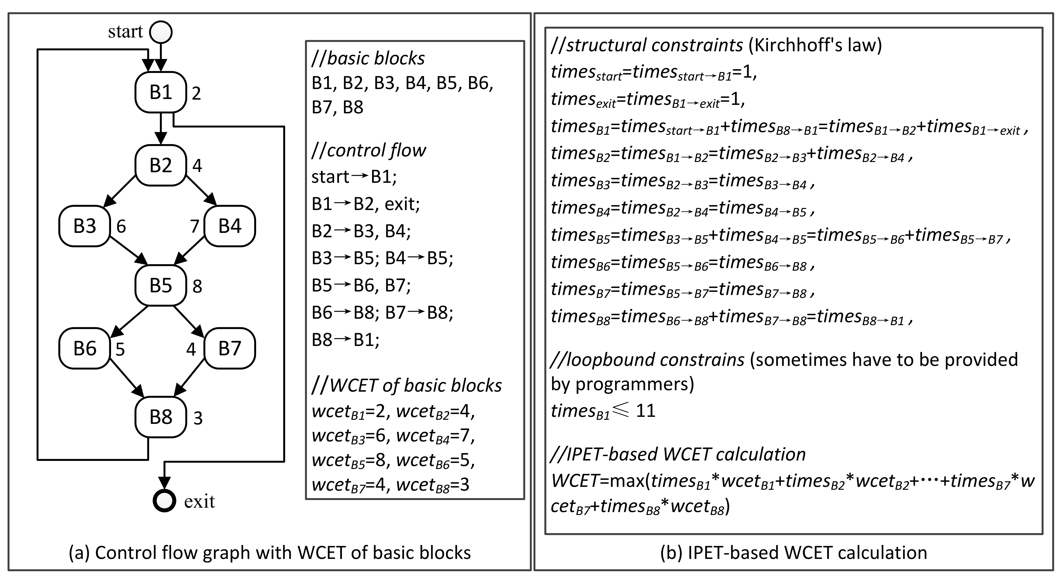
As a classical approach, IPET-based WCET analysis commonly has three basic steps [24]: (1) Micro-architecture modeling (or called low-level analysis), regarding pipeline, cache, branch predictor and cycle-accurate timing, etc.; (2) Control-flow Analysis (or called high-level analysis), such as control-flow reconstruction [25,26], loop bound analysis [27,28], etc.; (3) WCET Calculating, using integral linear programming (ILP) to compute a final result. Figure 1 shows the principle of IPET-based WCET analysis, including a control-flow graph (CFG) generated by high-level analysis and IPET-based WCET calculation.
Definition 1.
(Control Flow Graph [29]) a control flow graph G = (V, E) in which V is the set of all nodes and E is the set of all edges. Each node v ∈ V is a basic block, and each edge e ∈ E connects two nodes vi, vj ∈ V.
3.1. Overestimation in Micro-Architecture Modeling
IPET (implicit path enumeration technique) [31,32] is to establish a series of linear constraints for execution counts of each basic block according to the CFG, and then calculate the maximum execution time by ILP (see Equation (1)). Note that a basic block is a piece of sequential instructions. Only the last instruction can be a jump instruction and only the first instruction can be a jump target.
where, B denotes a basic block in the CFG; B denotes the set of all basic blocks; is the execution counts of basic block B; is the WCET of basic block B.
Usually, can be obtained from the low-level analysis, while needs to be calculated with some given flow constraints, and the goal is to maximize WCET. From the Equation (1), it is easy to see that WCET overestimation may come from both micro-architecture modeling and control-flow analysis.
For micro-architecture modeling abstract interpretation [33,34,35] has a dominant position. It uses cache behavior classification (i.e., always hit, always miss, first miss, not classified, etc.) to abstractly express the actual situation of instruction fetch [36]. The advantage is that state-explosion problems can be solved. However, since all non-classified cache behaviors are treated as always miss, the fetching time of many instructions is magnified [37]. Consequently, is overestimated. It is the most common reason for WCET overestimation.
3.2. Overestimation in Control-Flow Analysis
Normally, can be calculated by using ILP. The calculation needs some flow constraints which can be generated on the basis of Kirchhoff's law, see Equation (2). In addition, users may have to manually provide some linear constraints to express loop bounds and any infeasible path information.
where, denotes the counts control flow goes through the CFG edge ; denotes the counts control flow goes through the CFG edge .
In this article, loop bound refers to the maximum iteration counts of a loop statement. For a loop nesting, denoted , the loop bound of an inner loop is usually expressed as a constraint relationship relative to its outer loop. Take the following code as an example (Example 1). Obviously, the loop bound of outer for loop (denoted ) is 5. The loop bound of inner for loop (denoted ) is 25, and it can be expressed as , since executes five times in every execution of . However, for non-orthogonal nested loop, the relationship of maximum iteration counts between inner loop and outer loop is unclear.
| Example 1. A loop nesting with an orthogonal nested loop |
| 1 for ( int i = 0; i < 5; i++) |
| 2 for ( int j = 0; j < 5; j++) |
| 3 { k++; } |
Definition 2.
(Orthogonal Nested Loop) For a loop nesting , if always has the same execution counts during every execution of , then loop is called an orthogonal nested loop.
For an orthogonal nested loop, its loop control variable is context free. Note that the concept of non-orthogonal nested loop is opposite to orthogonal nested loop. In this paper, if the iteration counts of a nested loop (i.e., inner loop) are wholly or partly dependent on the variables modified by the outside loop, then the inner loop is called “non-orthogonal” nested loop.
Set the following program as an example (Example 2). The maximum iteration counts of inner while (Line 8) not only depend on control variable i (Line 7, j = i), but also are relevant to the values of array a. Thus, it is a typical non-orthogonal nested loop.
| Example 2. insertsort.c derived from WCET benchmarks (http://www.mrtc.mdh.se/projects/wcet/benchmarks.html) |
| 1 unsigned int a[11]; |
| 2 int main () |
| 3 { int i, j, temp; |
| 4 a[0] = 0; a[1] = 11; a[2] = 10; a[3] = 9; a[4] = 8; a[5] = 7; a[6] = 6; a[7] = 5; a[8] = 4; a[9] = 3; a[10] = 2; |
| 5 i = 2; |
| 6 while(i <= 10) |
| 7 { j = i; |
| 8 while (a[j] < a[j − 1]) //append condition “j <= 3” or “j <= 5” in Section 3 |
| 9 { temp = a[j]; a[j] = a[j − 1]; a[j − 1] = temp; j--; } |
| 10 i++; |
| 11 } |
| 12 return 1; |
| 13 } |
Considering the inner while loop runs at most nine times when the outer while loop runs once, to ensure safety, a pessimistic constraint can be used to express the loop bound of inner while loop. Since the iteration count of outer while loop is 9, the inequality makes the maximum iteration counts of inner while loop up to 81. However, the maximum iteration counts of inner while loop actually are 45, which is 1 + 2 + 3 + 4 + 5 + 6 + 7 + 8 + 9 = 45. Therefore, a pessimistic constraint results in a WCET overestimation since of inner while loop is enlarged. To solve this overestimation problem, an absolute constraint can be appended according to the global maximum iteration counts of inner while. Then the WCET overestimation will be reduced.
Definition 3.
(Pessimistic Constraint) pessimistic constraint refers to the loop bound of a nested loop statement expressed as the form , where and is the execution counts of the nested loop statement when its outer loop statement runs one time.
Definition 4.
(Absolute Constraint) absolute constraint refers to the loop bound of a nested loop statement expressed as the form , where is the total execution counts of the nested loop statement when the whole program runs one time.
4. Specific WCET Overestimation
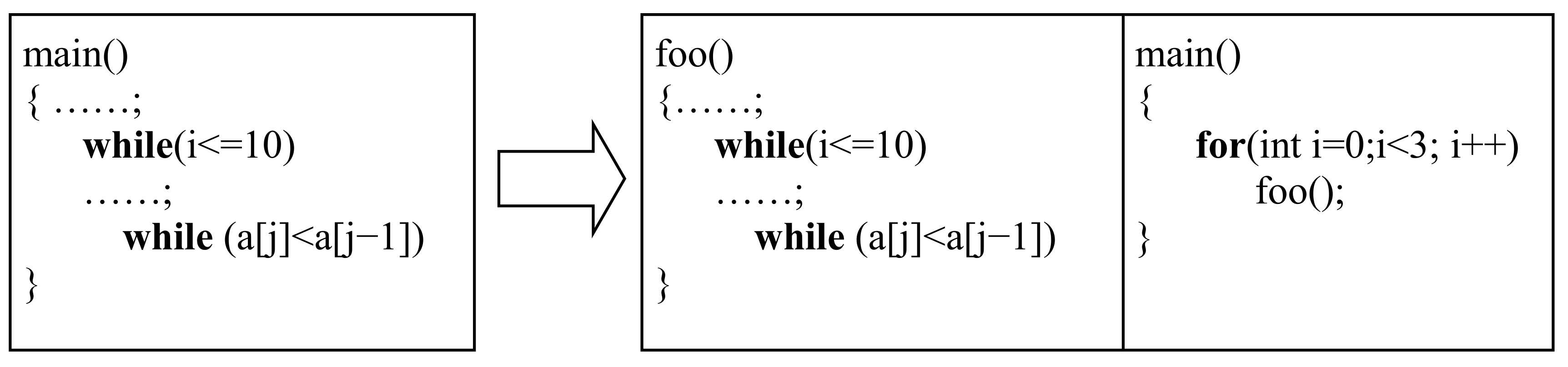
Supposing that the program in Example 2 was merely a part (or a function) of a long and complex program. For example, rename main () to foo (), and write a new main () which invokes foo () three times by a loop, see Figure 2. As a result, 45 was no more the global maximum iteration counts of inner while loop. So the constraint was no more correct, and it should be . To keep the useful knowledge of control flow, the local maximum iteration counts can be transformed into a new relative constraint . It is because the local maximum iteration counts of outer while loop are 9, and 45 ÷ 9 = 5. On the basis, since , the actual global maximum iteration counts of inner while loop will be .
Definition 5.
(Relative Constraint) relative constraint refers to the loop bound of a nested loop statement expressed as the form , where and , respectively is the execution counts of the nested loop statement and the outer loop statement when some function runs one time.
Table 1 shows the WCET estimations obtained by using different constraints. Note that the experimental tool is Chronos (http://www.comp.nus.edu.sg/~rpembed/chronos/). Target processor is simple without cache and other complex architecture. The optimization level of compiler is O1. The experimental results on “insertsort” show that the relative constraint (Col. 3) has the same effect as the absolute constraint (Col. 4). They all reduce the overestimation caused by the pessimistic constraint (Col. 2).
However, not all non-orthogonal nested loops can transform their local maximum iteration counts into a relative integral constraint. For example, respectively replace the conditional expression “a[j] < a[j − 1]” of second while loop in Example 2 with “j <= 3 && a[j] < a[j − 1]” and “j <= 5 && a[j] < a[j − 1]” to generate two new programs, named insertsort01 and insertsort02. For insertsort01, the local maximum iteration counts of second loop are three. For insertsort02, the local maximum iteration counts of second loop are ten. Both of them are not an integral multiple of their outer loop. The first one is 3/9, and the second one is 10/9.
In this situation, since WCET calculation relies on ILP, and ILP only handles integral constraint, a potential WCET overestimation emerges. Take insertsort01 as an example, one is the integer which is bigger than and the closest to the actual constraint value 3/9. Thus, the relative constraint for the second loop can be expressed as . Consequently, estimating WCET with the constraint generates an overestimation, see second row in Table 1 (324 > 228). Note that, for insertsort01, pessimistic constraint is since inner loop statement runs at most 2 times when outer loop statement runs once; absolute constraint is since the global maximum iteration counts of inner loop are 3. For insertsort02, pessimistic constraint is , relative constraint is , and absolute constraint is .
This kind of overestimation is neither caused by imprecise micro-architecture analysis nor brought by unfaithful control-flow analysis. It is an inherent imperfection of IPET-based WCET calculation. To overcome the disadvantage, at least quickly find and partly correct the overestimation, the general existence conditions of the specific WCET overestimations are firstly proposed. Without loss of generality, the programs which have the specific WCET overestimations need to satisfy the following conditions:
Firstly, . Where denotes the set of all non-orthogonal nested loops in a program P, and denotes the set of all statements which lie in the WCEP of P. This condition means that there is at least one non-orthogonal nested loop in the WCEP.
Secondly, only relative constraint is available. Many reasons can result in this situation, such as, the program is long and complex, and/or the development is not yet completed. Thus, it is hard to analyze the global maximum iteration counts. However, if the outer loop is orthogonal, like “for ( int 0; 5; i++)”, local maximum iteration counts of the inner non-orthogonal nested loop can be analyzed and obtained, for instance, by using program slicing [21].
Thirdly, . Where and respectively denote the local loop bounds of the outer and inner loop statements. Note that is an unsigned modulo operator.
5. Reducing Unreasonable Overestimation
To fundamentally eliminate the specific unreasonable WCET overestimation, the program must not have at least one of the above three conditions. However, it is unrealistic because the structure and the features of a program are mainly determined by the realistic demands. The code should directly reflect the program’s function. Intentionally changing the code’s structure to destroy the conditions will reduce the readability, or even bring bugs into the code. Therefore, in this article we do not research how to fundamentally eliminate the overestimation, but try our best to safely and effectively reduce the overestimation by improving the WCET calculation.
5.1. The Correction Example
In order to more clearly introduce the algorithm, firstly, the issue is simplified as: the program P only has one loop nesting whose depth is 2, and the non-orthogonal nested loop is not contained by any branch statement. Example 3 can reduce the WCET overestimation of P.
| Example 3. Reducing WCET overestimation for one non-orthogonal nested loop |
| Input: Program P with an non-orthogonal loop nesting {} |
| Output: Corrected WCET |
| 1: |
| 2: Set Constraint For Inner Loop () |
| 3: WCET1 ← WCET Analyse (P) |
| 4: |
| 5: Set Constraint For Inner Loop () |
| 6: WCET2 ← WCET Analyse (P) |
| 7: |
| 8: |
| 9: |
| 10: Return WCET |
Make insertsort01 mentioned in Section 4 as an example to explain the algorithm. = 9 and = 3, thus = 1 and = 2. Since the constraints and are the same as the constraints used in Section 4, we can see from Table 1 that WCET1 is 324 (Relative) and WCET2 is 468 (Pessimistic). Then error will be 16 and the corrected WCET will be 228. Note that the result is the same as the result obtained by using the absolute constraint . Using the algorithm, the WCET overestimation in insertsort02 can also be reduced.
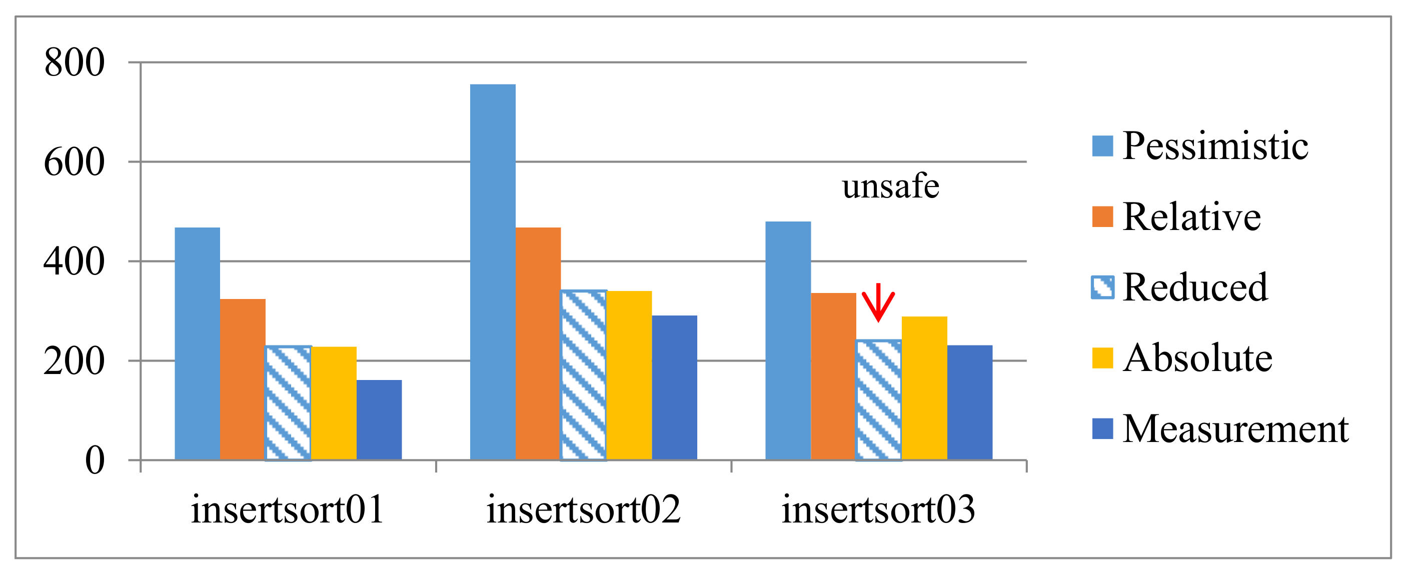
The reducing effects on insertsort01 and insertsort02 are shown in Figure 3. The two reduced WCET values are safe because both of them are no less than the WCET calculated from the absolute constraints. However, the result may be unsafe when the restrictions presupposed at the beginning of this section are removed, see insertsort03 in Figure 3.
Note that, insertsort03 is derived from program “insertsort”. Its structure is simply shown as Example 4. The loop nesting is moved into then part of a branch. The same or indifferent parts are omitted. Program insertsort03 has two mutually exclusive paths: path1 = <1,2,3,6> and path2 = <1,4,5,6>. In fact, the correct WCEP is path2. However, since a relative constraint has to be used for the loop at line 3, the WCEP switches to path1 from path2. Then the WCET correction is conducted on path1, and finally the reduced WCET becomes less than the correct WCET which belongs to path2. That is the reason why the above method may be unsafe when the non-orthogonal nested loop lies in a branch statement. To handle the more common cases, Section 5.2 introduces the whole process of the WCET corrections.
| Example 4. insertsort03.c derived from insertsort |
| 1 if ( … ) |
| 2 while ( i <= 10){ j = i; |
| 3 while ( j <= 3 && a[j] < a[j − 1]) {…}…} |
| 4 else //the correct WCEP |
| 5 {…} |
| 6 … |
5.2. The Whole Process
To avoid a wrong correction caused by WCEP switch during reducing WCET overestimation, the correction is limited to the non-branching part of WCEP. Note that the non-branching part refers to the code (i.e., the non-orthogonal nested loop) which does not belong to any branch statement. It means that the non-branching part of WCEP is a public sub-path that all execution traces must pass. So, no path switches can happen during reducing WCET overestimation.
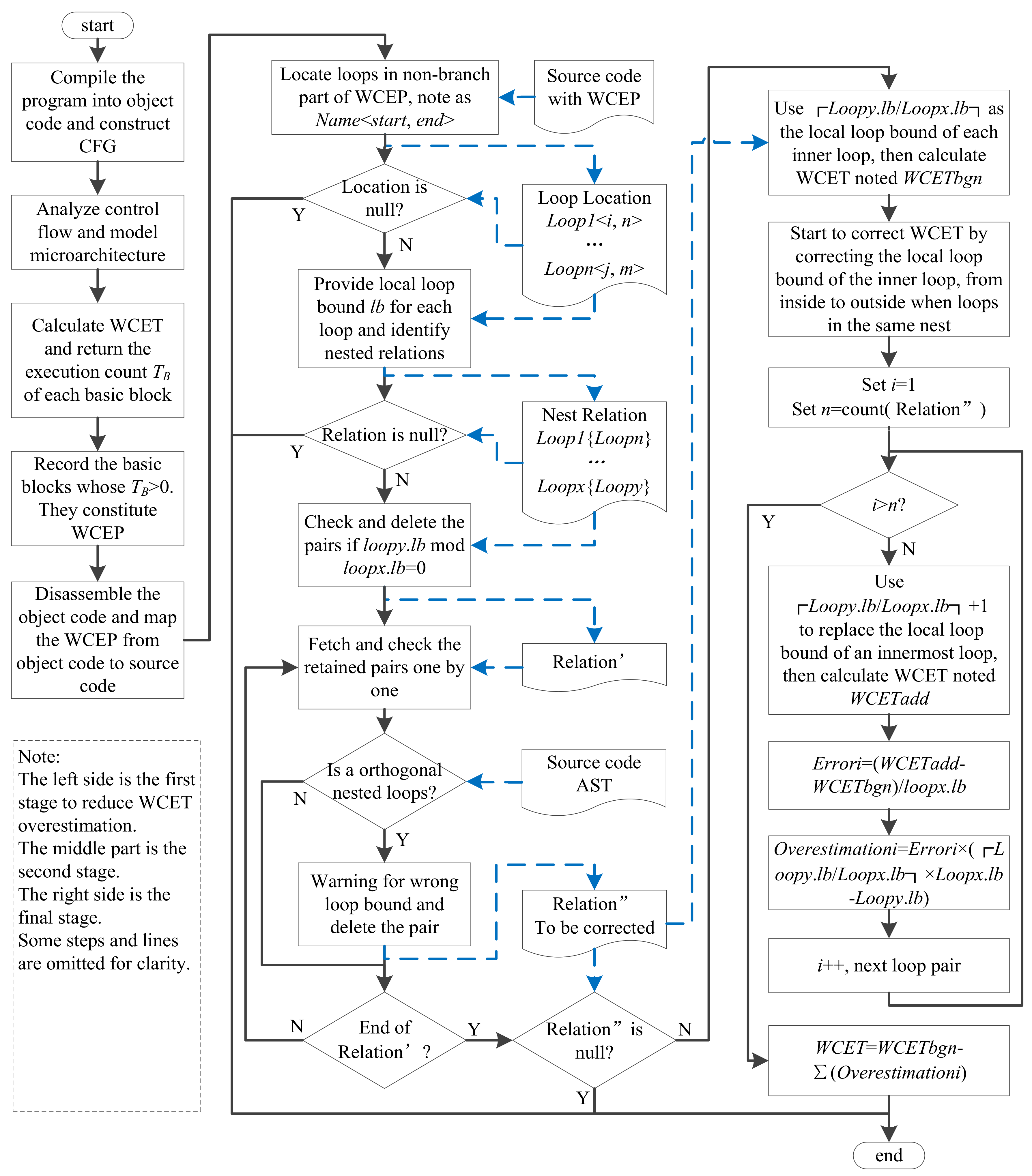
The WCET overestimation correction has three stages The first stage is to locate WCEP in CFG and then map it onto source code. The second stage is to identify the non-orthogonal nested loops in WCEP by means of abstract syntax tree (AST). The last stage is to recursively calculate the WCET errors caused by the loose constraint relationships of loop bounds, and reduce the WCET overestimation via subtracting the total errors. Figure 4 shows the whole process of our WCET correction.
In the first stage, the variable values of ILP (i.e., in Equation (1)) are used to locate WCEP. For a basic block , if its execution counts in the final result, then belongs to WCEP. So, it is easy to locate all basic blocks which constitute WCEP. Note that using different constraints (i.e., pessimistic, relative or absolute) to express the maximum iteration counts of nested loops may result in different WCEP. However, it is unconsidered since our approach only deals with a non-branching part, and the part is always the same even in different WCEP.
In the second stage, two ways can achieve identifying nested relations. The first way (showing in Figure 2) is using the start and end line information. Generally, for two loops (denoted loopx and loopy respectively), if loopx.start_line < loopy.start_line and loopx.end_line > loopy.end_line, then loopy is nested by loopx. The second way identifies nested relations with the help of AST. When the nodes of loopy are children of the node of loopx, then loopx nests loopy.
To identify the non-orthogonal nested loops, and help programmers analyze loop bounds, we have developed a lightweight syntax analysis tool for C language (supporting C99 standard), called CParser [38]. Through three basic steps, i.e., lexical analysis, preprocessing and syntax analysis, CParser not only creates AST, but also identifies non-orthogonal nested loops. Meanwhile, by means of source code instrumentation, CParser provides referential loop bounds for programmers. Moreover, CParser has also been used in error locating of C programs [39]. Usually manual analysis is inevitable to obtain loop bounds since other methods, such as symbolic execution, have many limitations in availability. Therefore, the referential loop bounds are beneficial for making sure that the loop bounds provided by programmers are not smaller than the actual values.
It should be noted that, a non-orthogonal nested loop may not necessarily be the object of the correction unless its local maximum iteration counts are not integral multiples relative to its outer loop. Meanwhile, orthogonal nested loop must meet the integral multiple relations. So, if the provided local loop bound for orthogonal nested loops does not meet the integral multiple relations, the annotations for local maximum iteration counts must be wrong.
In the final stage, if the depth of a loop nesting is more than two, the correction will start from the innermost loop. For example, for two loop nests Loopx {Loopy} and Loopy {Loopz}, obviously Loopz is the innermost loop, so our approach corrects Loopy {Loopz} first. Otherwise, it will result in new errors during Loopx {Loopy} correction.
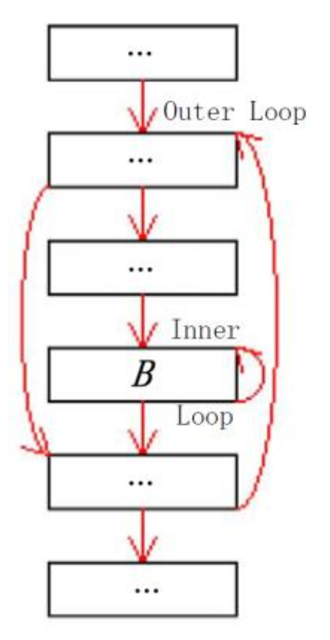
5.3. The Safety Analysis
If the reduced WCET (denoted RWCET) is no less than the WCET which is calculated by using absolute constraints (denoted WCET), then the correction algorithm must be safe. For making the safety analysis easy to be understood, we suppose that the program has a CFG which is simply shown in Figure 5. It should be pointed out that the correction only affects the total execution time of the basic block (denoted ). Therefore, the question is simplified as: if then the correction algorithm is safe. Where is the total WCET of the basic block B after correction. According to Equation (1), . Therefore, if then the algorithm is safe.
For a loop nesting , supposing their max execution counts respectively are and . We firstly prove the safety of the algorithm without considering Cache.
Proof.
According to the Example 1, obviously , and , so we have , and .
Obviously, .
Since , now we have , which completes the proof. ☐
When considering cache, the basic block B has two kinds of execution time: for Cache hit and for cache miss. So . According to the classification of cache behaviors, the safety is analyzed from three aspects. Firstly, if B is always hit, then . Thus . The proof under this case is the same with the previous one, so we don’t repeat it. Secondly, if B is always miss, then . Therefore . The proof under this case is also the same with the previous one. Thirdly, if B is first miss, then it has two cases. If , then and , so ; if , then and , so . Following is the proof in the third case.
Proof.
According to the Example 1, obviously , and .
So we have , and .
Obviously, .
If , then ;
If , then
Since and , we have ☐
Summing up the above, is always true. Therefore, the WCET correction algorithm is safe. Note that the inner loop may have many basic blocks and the processor may have other configurations, such as data cache and pipeline, but the theory is similar. Thus, the safety, when considering more details, can also be proved using the same method. However, the algorithm is only the kernel of the whole correction process. Even if it is safe, it does not mean that the whole process must be safe since the whole process involves identifying correctable non-orthogonal nested loops and other details. For example, if a programmer provides wrong loop bounds, any safe approach including our correction cannot guarantee safety.
6. Evaluation
Generally, WCET estimation is evaluated from two aspects: safety and accuracy. Therefore, the purpose of this section is to answer the following questions: (1) From a practical perspective, is the corrected WCET estimation by our approach is still safe?; (2) How about the effectiveness of our approach in improving the accuracy of WCET overestimation?; (3) Which factors may threaten the safety and effectiveness of our approach? Questions 1 and 2 are answered in Section 6.3, and Question 3 is discussed in Section 6.4.
6.1. Experimental Setup
Experimental tools: Chronos and CParser. Chronos is a well-known WCET analysis tool, and it can easily set and change the configuration of micro-architecture. Due to the flexibility, we used Chronos to analyze programs on different target processors. CParser has been introduced in Section 5.2.
Experimental programs: ten programs shown in Table 2. “Statement” refers to the number of statements in the program. “NNloop” denotes the number of non-orthogonal nested loops. “Correctable” expresses the number of the non-orthogonal nested loops which lie in non-branch part of WCEP. “Depth” indicates the max depth of the “correctable” nested loop.
Compiler was GCC, and the optimization level was O1. The experiments were conducted on a simple target processor and a complex processor, respectively.
6.2. Experimental Results
Table 3 shows the results when the processor is simple. The simple processor has no cache and branch predictor. Thus, the WCET overestimation only comes from the loose or wrong loop bound constraints. “Reduced” in Table 3 and Table 4 refer to the WCET after the correction.
Table 4 shows the results when the processor is complex. The complex processor has cache, branch predictor and out-of-order pipeline (see Table 5). Thus, the WCET overestimation is more real. Note that, when using complex processor, Chronos did not calculate the WCET for program minver. This is not a rare situation since IPET-based WCET calculation is a NP-hard problem. ILP sometimes runs very slowly, and it even cannot return a result when the program has a complex structure.
6.3. Analysis
6.3.1. Safety
A reduced WCET (denoted Rwcet) is safe only when Rwcet Cwcet. Where Cwcet denotes the correct WCET calculated by using absolute constraints. Table 6 shows the difference values obtained from Rwcet-Cwcet on different processors.
It clearly shows that reduced WCET of 100% are no less than correct WCET. Therefore, both the experimental results and the theoretical analysis in Section 5.3 support the conclusion that our approach including the algorithm and the whole process is safe. Therefore, the answer to Question 1 is affirmative.
6.3.2. Effectiveness
Figure 6 shows the average ratios of different WCET overestimations relative to the correct WCET. The ratios for pessimistic WCET are up to 259.65% and 128.29%. The ratios for relative WCET are 17.24% and 6.74%. Oppositely, the ratios for reduced WCET are only 1.56% (on simple processor) and 1.05% (on complex processor). From an overall perspective, our approach has obvious effects on reducing the WCET overestimations. Note that the ratio of overestimation for a program is calculated by Equation (3).
where, Cwcet denotes the correct WCET; Owcet can be pessimistic, relative or reduced WCET.
Here, we continue to analyze the effects on each program. Equation (4) was used to calculate the percentage of WCET reduction, where Owcet and Rwcet have the same meaning with Equation (3). Figure 7 and Figure 8, respectively, show the reductions of WCET overestimations on simple processor and complex processor.
It can be easily seen that both pessimistic WCET and relative WCET are reduced by our approach. The percentage of reductions is at least 82% on average. Summing up the above, Question 2 is answered here: that our approach can obviously reduce the specific WCET overestimations, and thus, increase the accuracy of WCET estimation.
6.3.3. Efficiency
Since our approach needs to calculate WCET at least twice for reducing the overestimations, it costs more time than IPET-based WCET estimation. Figure 9 shows the comparisons of the two methods in time cost.
6.4. Discussion
6.4.1. Threat to Safety
The safety of the WCET correction has been proved in Section 5.3 and verified in Section 6.3.1. The fundamental guarantee of safety is that WCET correction is only conducted on the non-branching part of WCEP, thus, no WCEP switches happen. In fact, our approach may safely reduce the specific WCET overestimation even if the non-orthogonal nested loop lies in the branching part of WCEP. For instance, Table 7 shows the results of WCET correction on program “select”. Note that all non-orthogonal nested loops lie in branch statements.
The correction is safe because the non-orthogonal nested loops lie in the invariant path [40] of WCEP. Actually, invariant path is a concept in the field of code optimization for reducing WCET, and it includes various cases. Therefore, to ensure the absolute safety, our approach did not enlarge the scope of correction. Obviously, our approach is conservative but safe, and the safety is almost not threatened by anything (except if the developer provides wrong local max iteration counts).
6.4.2. Threat to Effectiveness
Regarding Question 3, three factors can threaten the validity of the experimental results as well as the effectiveness of our approach. The first is micro-architecture of target processor. The second is control flow of the sample program. The third is the optimization level of compiler.
Differences in micro-architecture result in different WCET estimation, and then, the overestimation is reduced with different percentages. Comparison of Figure 7 and Figure 8 clearly shows that our approach obviously has different effectiveness in reducing overestimation (for example, program insert02) on different processors. Therefore, to keep the validity, our experimental results were obtained on two different types of processors.
For the program ludcmp and minver, since not all non-orthogonal nested loops lie in the non-branching part of WCEP, our approach can only correct a part of overestimation for ensuring safety. Theoretically, the more non-orthogonal nested loops lie in branch statements, the less the percentage of overestimation is reduced. Thus, our experiment tried to adopt samples derived from different benchmark programs for supporting the validity. The number of programs which derived from the same origin was no more than two.
Compiler optimization is usually used to increase the average performance. However, it does not always improve WCET with the rise of optimization level. For instance, O2 optimization even made a larger WCET than O1 optimization on program bsort (see Figure 10). Meanwhile, considering O2 optimization significantly modified the object code, and thus, accurately mapping WCEP from object code onto source code became difficult. To avoid excessive optimization, our experiment used O1 optimization.
7. Conclusions
Classical IPET-based WCET analysis cannot avoid a kind of specific overestimation. The overestimation comes from neither micro-architecture modeling nor control flow analysis. It occurs because ILP-based WCET calculations cannot handle non-integer loop bound constraints. To reduce specific WCET overestimation, three basic existence conditions were proposed, and then a correction approach was developed. The correction approach firstly locates WCEP in CFG and then maps it onto source code. Secondly it identifies the non-orthogonal nested loop in the WCEP by means of AST. Finally, the WCET overestimation is corrected via subtracting the total errors.
The experimental results show that the specific overestimations are reduced more than 82% on average, and all the corrected WCET estimations are safe. It will help programmers to obtain more precise WCET estimation, and then design more safe and efficient real-time systems [41,42,43]. The disadvantage of our approach is that it requires repeatedly analyzing and calculating WCET; therefore, it is more time-consuming than the IPET-based WCET analysis. In the future, attention will be focused on multi-core processors. Whether the specific WCET overestimation can also occur on multi-core processor, and the safety and availability of our approach when target processor is multi-core are issues that are worthy of further study.
Acknowledgments
This work was supported by “the 13th Five-Year” National Science and Technology Major Project of China (Grant No. 2017YFC0702204), the national natural science foundation of China (No. 61672191 and No. 61173021).
Author Contributions
Fanqi Meng and Xiaohong Su conceived and designed the experiments; Fanqi Meng performed the experiments; Fanqi Meng and Xiaohong Su analyzed the data; Fanqi Meng wrote the paper.
Conflicts of Interest
The authors declare no conflict of interest.
References
- Zhu, D.; Aydin, H. Reliability-aware energy management for periodic real-time tasks. IEEE Trans. Comput. 2009, 58, 1382–1397. [Google Scholar]
- Aydin, H.; Devadas, V.; Zhu, D. System-level energy management for periodic real-time tasks. In Proceedings of the 27th IEEE International Real-Time Systems Symposium (RTSS’06), Rio de Janeiro, Brazil, 5–8 December 2006; pp. 313–322. [Google Scholar]
- Zou, C.; Hu, X.; Wei, Z.; Tang, X. Electrothermal dynamics-conscious lithium-ion battery cell-level charging management via state-monitored predictive control. Energy 2017, 141, 250–259. [Google Scholar] [CrossRef]
- Li, X.; Liang, Y.; Mitra, T.; Roychoudhury, A. Chronos: A timing analyzer for embedded software. Sci. Comput. Program. 2007, 69, 56–67. [Google Scholar] [CrossRef]
- Wilhelm, R.; Engblom, J.; Ermedahl, A.; Holsti, N.; Thesing, S.; Whalley, D.; Bernat, G.; Ferdinand, C.; Heckmann, R.; Mitra, T.; et al. The worst-case execution-time problem—Overview of methods and survey of tools. ACM Trans. Embed. Comput. Syst. 2008, 7, 36. [Google Scholar] [CrossRef]
- Moreno, C.; Fischmeister, S. Accurate Measurement of Small Execution Times—Getting Around Measurement Errors. IEEE Embed. Syst. Lett. 2017, 9, 17–20. [Google Scholar] [CrossRef]
- Reineke, J.; Wilhelm, R. Static Timing Analysis–What is Specific? In Semantics, Logics, and Calculi; Springer: New York, NY, USA, 2016; pp. 74–87. [Google Scholar] [CrossRef]
- Cousot, P.; Cousot, R. Abstract interpretation: A unified lattice model for static analysis of programs by construction or approximation of fixpoints. In Proceedings of the 4th symposium on Principles of Programming Languages ACM SIGACT-SIGPLAN, Los Angeles, CA, USA, 17–19 January 1977; pp. 238–252. [Google Scholar] [CrossRef]
- Martin, F.; Alt, M.; Wilhelm, R.; Ferdinand, C. Analysis of loops. In Proceedings of the 7th International Conference on Compiler Construction, Lisbon, Portugal, 30 March–3 April 1998; pp. 80–94. [Google Scholar]
- Ballabriga, C.; Casse, H. Improving the first-miss computation in set-associative instruction Caches. In Proceedings of the 2008 Euromicro Conference on Real-Time Systems, Prague, Czech Republic, 2–4 July 2008; pp. 341–350. [Google Scholar] [CrossRef]
- Ferdinand, C.; Wilhelm, R. On predicting data Cache behavior for real-time systems. In Proceedings of the ACM Sigplan Workshop on Languages, Compilers, and Tools for Embedded Systems, Montreal, QC, Canada, 19–20 June 1998; pp. 16–30. [Google Scholar] [CrossRef]
- Sen, R.; Srikant, Y.N. WCET estimation for executables in the presence of data Caches. In Proceedings of the 7th ACM & IEEE International Conference on Embedded Software, Salzburg, Austria, 30 September–3 October 2007; pp. 203–212. [Google Scholar] [CrossRef]
- Gustafsson, J.; Ermedahl, A.; Sandberg, C.; Lisper, B. Automatic derivation of loop bounds and infeasible paths for WCET analysis using abstract execution. In Proceedings of the 27th IEEE International Real-Time Systems Symposium, Rio De Janeiro, Brazil, 5–8 December 2006; pp. 57–66. [Google Scholar] [CrossRef]
- Healy, C.; Whalley, D. Automatic detection and exploitation of branch constraints for timing analysis. IEEE Trans. Softw. Eng. 2002, 28, 763–781. [Google Scholar] [CrossRef]
- Bernard, B.; Gernot, H. Sequoll: A Framework for Model Checking Binaries. In Proceedings of the 2013 IEEE 19th Real-Time and Embedded Technology and Applications Symposium (RTAS), Philadelphia, CA, USA, 9–11 April 2013; pp. 97–106. [Google Scholar] [CrossRef]
- Knoop, J.; Kovács, L.; Zwirchmayr, J. Symbolic loop bound computation for WCET analysis. In Proceedings of the International Andrei Ershov Memorial Conference, Novosibirsk, Russia, 27 June–1 July 2011; pp. 227–242. [Google Scholar] [CrossRef]
- Knoop, J.; Kovács, L.; Zwirchmayr, J. Replacing conjectures by positive knowledge: Inferring proven precise worst-case execution time bounds using symbolic execution. J. Symb. Comput. 2017, 80, 101–124. [Google Scholar]
- King, J.C. Symbolic execution and program testing. Commun. ACM 1997, 19, 385–394. [Google Scholar] [CrossRef]
- Lokuciejewski, P.; Cordes, D.; Falk, H.; Marwedel, P. A fast and precise static loop analysis based on abstract interpretation, program slicing and polytope models. In Proceedings of the 7th International Symposium on Code Generation and Optimization, Seattle, WA, USA, 22–25 March 2009; pp. 136–146. [Google Scholar] [CrossRef]
- Maroneze, A.; Blazy, S.; Pichardie, D.; Puaut, I. A Formally Verified WCET Estimation Tool; OASIcs-Open Access Series in Informatics; Schloss Dagstuhl-Leibniz-Zentrum fuer Informatik: Saarbrücken, Germany, 2014; Volume 39, pp. 11–20. [Google Scholar] [CrossRef]
- Blazy, S.; Maroneze, A.; Pichardie, D. Formal verification of loop bound estimation for WCET analysis. In Working Conference on Verified Software: Theories, Tools, and Experiments; Springer: Berlin/Heidelberg, Germany, 2013; pp. 281–303. [Google Scholar] [CrossRef]
- Sewell, T.; Kam, F.; Heiser, G. Complete, High-Assurance Determination of Loop Bounds and Infeasible Paths for WCET Analysis. In Proceedings of the 2016 IEEE Real-Time and Embedded Technology and Applications Symposium (RTAS), Vienna, Austria, 11–14 April 2016; pp. 1–11. [Google Scholar] [CrossRef]
- Čadek, P.; Strejček, J.; Trtík, M. Tighter Loop Bound Analysis. International Symposium on Automated Technology for Verification and Analysis; Springer: New York, NY, USA, 2016; pp. 512–527. [Google Scholar] [CrossRef]
- Henry, J.; Asavoae, M.; Monniaux, D.; Maïza, C. How to compute worst-case execution time by optimization modulo theory and a clever encoding of program semantics. In Proceedings of the 2014 ACM SIGPLAN/SIGBED Conference on Languages, Compilers and Tools for Embedded Systems, Edinburgh, UK, 12–13 June 2014; pp. 43–52. [Google Scholar] [CrossRef]
- Theiling, H. Extracting safe and precise control flow from binaries. In Proceedings of the IEEE 7th International Conference on Real-Time Computing Systems and Applications, Cheju Island, Korea, 12–14 December 2000; pp. 23–30. [Google Scholar] [CrossRef]
- Kinder, J.; Zuleger, F.; Veith, H. An abstract interpretation-based framework for control flow reconstruction from binaries. In Verification, Model Checking, and Abstract Interpretation; Springer: Berlin/Heidelberg, Germany, 2009; pp. 214–228. [Google Scholar] [CrossRef] [Green Version]
- Healy, C.; Sjödin, M.; Rustagi, V.; Whalley, D.; van Engelen, R. Supporting timing analysis by automatic bounding of loop iterations. Real Time Syst. 2000, 18, 129–156. [Google Scholar] [CrossRef]
- Parsa, S.; Sakhaei-Nia, M. Modeling flow information of loops using compositional condition of controls. J. Supercomput. 2015, 71, 508–536. [Google Scholar] [CrossRef]
- Yousefi, J.; Sedaghat, Y.; Rezaee, M. Masking wrong-successor Control Flow Errors employing data redundancy. In Proceedings of the 2015 5th International Conference on Computer and Knowledge Engineering (ICCKE), Mashhad, Iran, 29 October 2015; pp. 201–205. [Google Scholar]
- Meng, F.; Su, X.; Qu, Z. Interactive WCET Prediction with Warning for Timeout Risk. Int. J. Pattern Recognit. Artif. Intell. 2017, 31, 1750012. [Google Scholar] [CrossRef]
- Li, Y.T.S.; Malik, S. Performance analysis of embedded software using implicit path enumeration. IEEE Trans. Comput. Aided Des. Integr. Circuits Syst. 1997, 16, 1477–1487. [Google Scholar] [CrossRef]
- Guan, N.; Lv, M.; Yi, W.; Yu, G. WCET analysis with MRU Cache: Challenging LRU for predictability. ACM Trans. Embed. Comput. Syst. 2014, 13, 123. [Google Scholar] [CrossRef]
- Boulanger, J.L. Static Analysis of Software: The Abstract Interpretation; John Wiley & Sons: Hoboken, NJ, USA, 2013. [Google Scholar]
- Cousot, P.; Cousot, R. Abstract interpretation: Past, present and future. In Proceedings of the Joint Meeting of the Twenty-Third EACSL Annual Conference on Computer Science Logic (CSL) and the Twenty-Ninth Annual ACM/IEEE Symposium on Logic in Computer Science (LICS), Vienna, Austria, 14–18 July 2014; p. 2. [Google Scholar] [CrossRef]
- Falaschi, M.; Olarte, C.; Palamidessi, C. Abstract interpretation of temporal concurrent constraint programs. Theory Pract. Log. Program. 2015, 15, 312–357. [Google Scholar] [CrossRef]
- Zhang, Z.; Koutsoukos, X. Improving the Precision of Abstract Interpretation Based Cache Persistence Analysis. In Proceedings of the 16th ACM SIGPLAN/SIGBED Conference on Languages, Compilers and Tools for Embedded Systems 2015 CD-ROM, Portland, OR, USA, 18–19 June 2015; p. 10. [Google Scholar] [CrossRef]
- Meng, F.; Su, X.; Qu, Z. Nonlinear approach for estimating WCET during programming phase. Clust. Comput. 2016, 19, 1449–1459. [Google Scholar] [CrossRef]
- Yang, S.; Su, X.; Wang, T.; Peijun, M.A. Design and Implementation of Lexical and Syntax Analysis Tool CParser for C Language. Intell. Comput. Appl. 2014, 5, 21. [Google Scholar]
- Su, X.; Wang, T.; Yang, S.J.; Ma, P.J. Fault localization based on weighted software behavior graph mining. Chin. J. Comput. 2016, 39, 2175–2188. [Google Scholar]
- Meng, F.; Su, X. WCET Optimization Strategy Based on Source Code Refactoring. Available online: https://link.springer.com/article/10.1007/s10586-017-1369-3 (accessed on 12 December 2017).
- Li, G.; Zhang, Y.; Zhang, M.; Zhang, L. The Wind Power Real-Time Diction on the EEMD and SVM of the MRMR. J. Northeast Electr. Power Univ. 2017, 37, 39–44. [Google Scholar] [CrossRef]
- Yang, M.; Huang, B.; Jiang, B.; Lin, S. Real-time Prediction for Wind Power Based on Kalman Filter and Support Vector Machines. J. Northeast Electr. Power Univ. 2017, 37, 46–51. [Google Scholar]
- Yang, M.; Yang, C. Research on Wind Power Real-Time Forecasting Based on Fuzzy Granular Computing. J. Northeast Electr. Power Univ. 2017, 37, 1–7. [Google Scholar]
Figure 1.
IPET-based WCET calculation [30].
Figure 1.
IPET-based WCET calculation [30].

Figure 2.
Modification of Example 2.

Figure 3.
WCET estimations obtained by using different constraints.

Figure 4.
The whole process of WCET overestimation correction.

Figure 5.
The control flow graph (CFG) of a program with non-orthogonal nested loop.

Figure 6.
The average ratio of WCET overestimation relative to correct WCET.
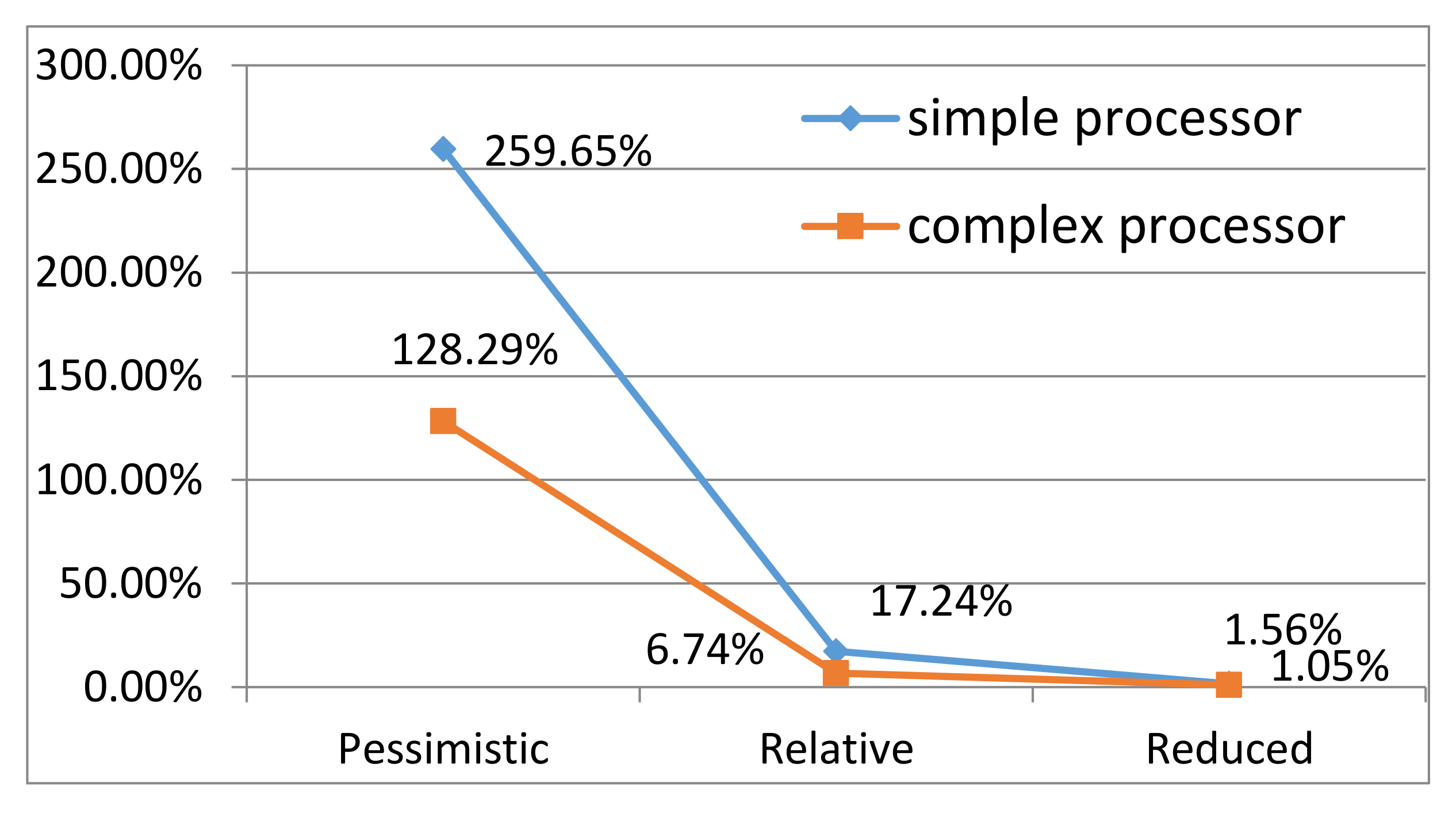
Figure 7.
The reductions of WCET overestimations on a simple processor.
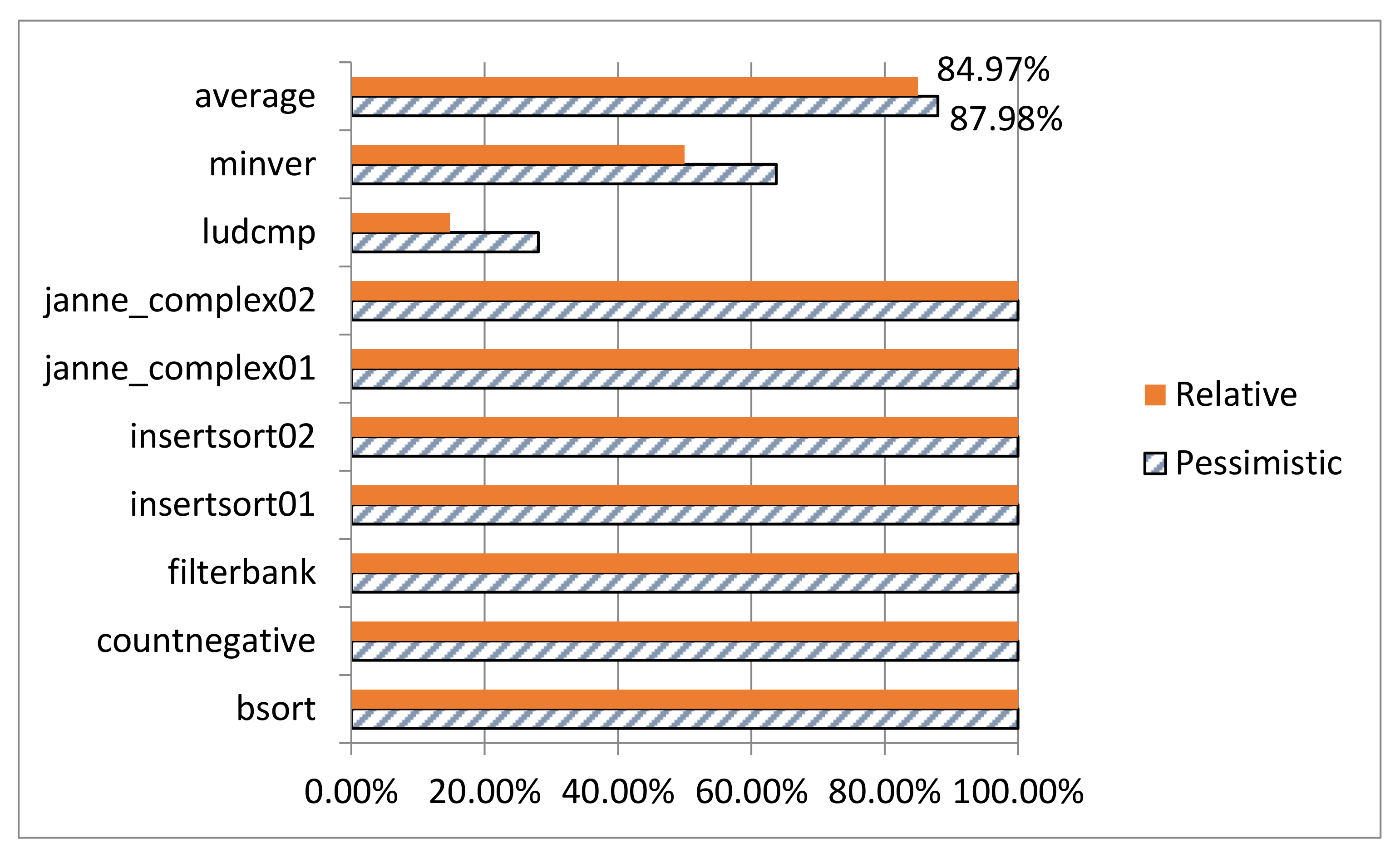
Figure 8.
The reductions of WCET overestimations on a complex processor.
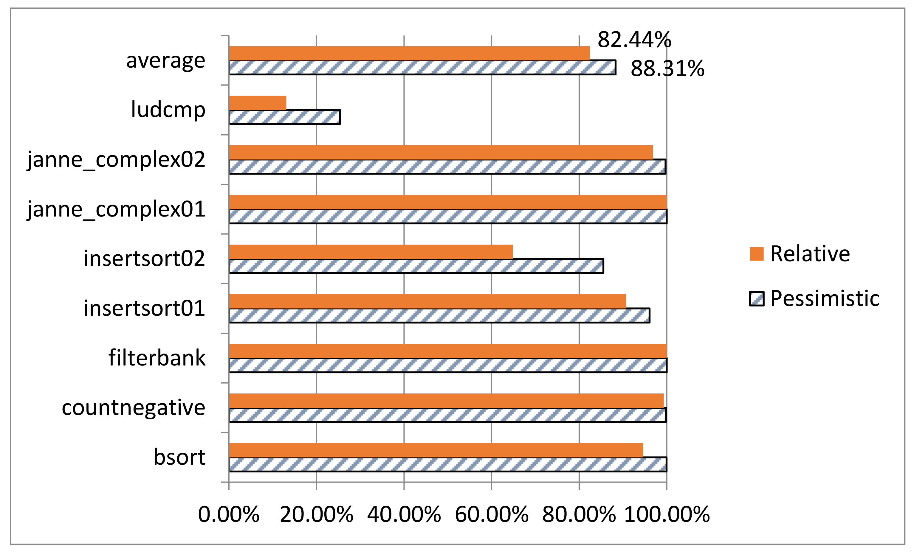
Figure 9.
The comparisons of time overhead.
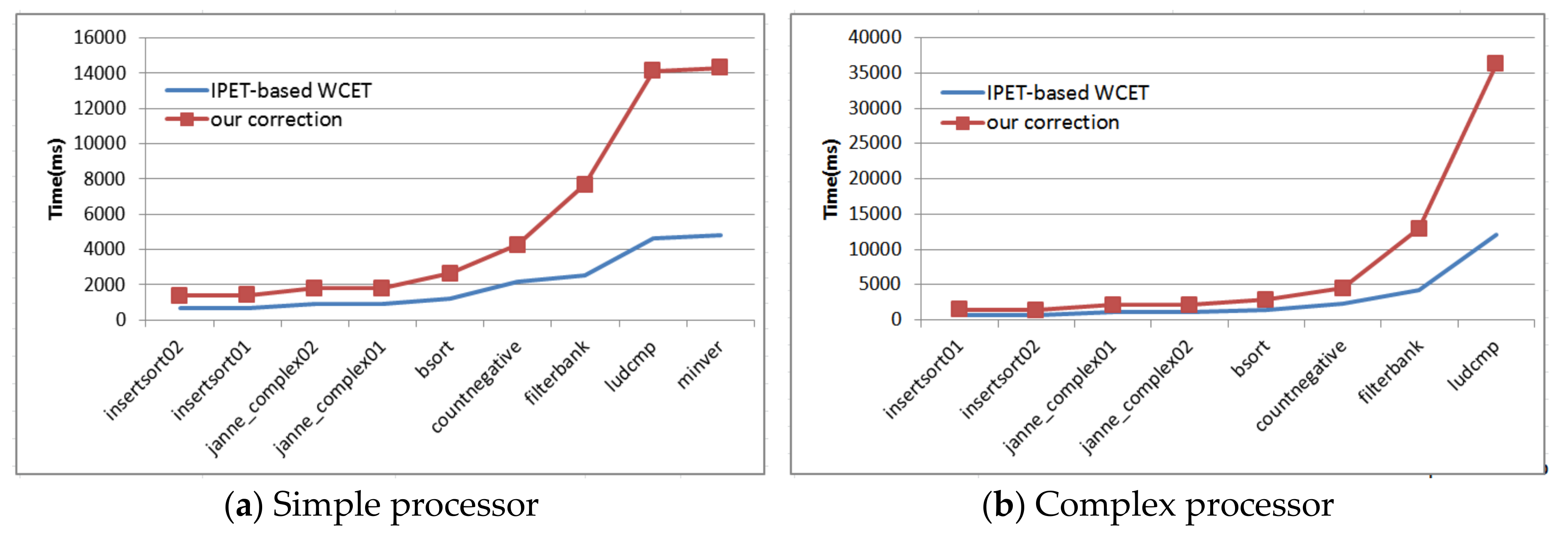
Figure 10.
The WCET obtained from different optimization levels of compiler (unit: cycle).

Table 1.
WCET estimations obtained by using different constraints (unit: cycle).
| Programs | Pessimistic | Relative | Absolute | Measurement |
|---|---|---|---|---|
| insertsort | 1863 | 1107 | 1107 | 1103 |
| insertsort01 | 468 | 324 | 228 | 161 |
| insertsort02 | 756 | 468 | 340 | 291 |
Table 2.
Experimental programs.
| Programs | Statement | NNloop | Correctable | Depth |
|---|---|---|---|---|
| bsort | 34 | 1 | 1 | 2 |
| countnegative | 56 | 1 | 1 | 2 |
| filterbank | 67 | 2 | 2 | 3 |
| insertsort01 | 27 | 1 | 1 | 2 |
| insertsort02 | 27 | 1 | 1 | 2 |
| janne_complex01 | 20 | 1 | 1 | 2 |
| janne_complex02 | 20 | 1 | 1 | 2 |
| ludcmp | 75 | 6 | 2 | 3 |
| minver | 102 | 4 | 2 | 3 |
| Select * | 27 | 3 | 0 | 3 |
Note: * denotes that no non-orthogonal nested loop lies in non-branch part of WCEP.
Table 3.
WCET obtained from different constraints on simple processor (unit: cycle).
| Programs | Pessimistic | Relative | Reduced | Absolute |
|---|---|---|---|---|
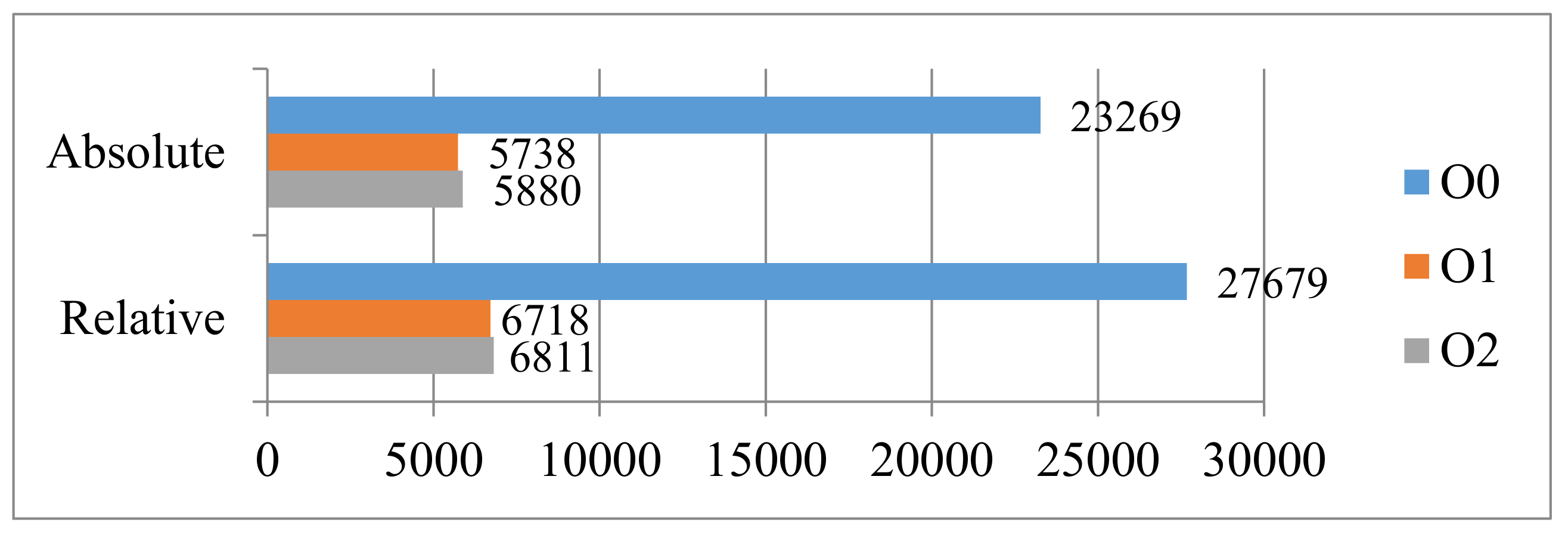
| bsort | 101,758 | 6718 | 5738 | 5738 |
| countnegative | 20,452 | 19,812 | 19,572 | 19,572 |
| filterbank | 4,171,890 | 4,044,910 | 3,925,870 | 3,925,870 |
| insertsort01 | 468 | 324 | 228 | 228 |
| insertsort02 | 756 | 468 | 340 | 340 |
| janne_complex01 | 2217 | 768 | 630 | 630 |
| janne_complex02 | 1390 | 631 | 556 | 556 |
| ludcmp | 6074 | 5944 | 5840 | 5240 |
| minver | 3558 | 3492 | 3405 | 3318 |
Table 4.
WCET obtained from different constraints on complex processor (unit: cycle).
| Programs | Pessimistic | Relative | Reduced | Absolute |
|---|---|---|---|---|
| bsort | 113,972 | 14,119 | 13,060 | 13,000 |
| countnegative | 21,410 | 20,630 | 20,338 | 20,336 |
| filterbank | 3,156,240 | 3,062,040 | 2,973,728 | 2,973,720 |
| insertsort01 | 1262 | 1115 | 1017 | 1007 |
| insertsort02 | 1445 | 1262 | 1179 | 1134 |
| janne_complex01 | 3967 | 2013 | 1827 | 1827 |
| janne_complex02 | 2853 | 1829 | 1736 | 1733 |
| ludcmp | 20,810 | 20,705 | 20,621 | 20,065 |
| minver | no result | no result | no result | no result |
Table 5.
The configuration of the complex processor.
| Item | Value |
|---|---|
| Pipeline parameters | out of order |
| Superscalarity | 2 |
| Instruction Fetch Queue Size | 4 |
| Reorder Buffer Size | 16 |
| Instruction Cache Parameters | Enable |
| Number of Sets | 16 |
| Block Size | 16 |
| Cache Associativity | 2 |
| Branch Prediction Parameters | Enable |
| Branch History Table Size | 32 |
| Branch History Register Width | 2 |
Table 6.
The difference between reduced WCET and correct WCET (unit: cycle).
| Programs | Simple Processor | Complex Processor |
|---|---|---|
| bsort | 0 | +60 |
| countnegative | 0 | +2 |
| filterbank | 0 | +8 |
| insertsort01 | 0 | +10 |
| insertsort02 | 0 | +45 |
| janne_complex01 | 0 | 0 |
| janne_complex02 | 0 | +3 |
| ludcmp | +600 | +556 |
| minver | +87 | unknown |
Table 7.
The results of WCET reduction on program “select” (unit: cycle).
| Processor | Relative | Reduced | Absolute | Difference |
|---|---|---|---|---|
| simple | 982 | 966 | 966 | 0 |
| complex | 12,735 | 12,713 | 12,707 | +6 |
© 2017 by the authors. Licensee MDPI, Basel, Switzerland. This article is an open access article distributed under the terms and conditions of the Creative Commons Attribution (CC BY) license (http://creativecommons.org/licenses/by/4.0/).
Share and Cite
MDPI and ACS Style
Meng, F.; Su, X. Reducing WCET Overestimations by Correcting Errors in Loop Bound Constraints. Energies 2017, 10, 2113. https://doi.org/10.3390/en10122113
AMA Style
Meng F, Su X. Reducing WCET Overestimations by Correcting Errors in Loop Bound Constraints. Energies. 2017; 10(12):2113. https://doi.org/10.3390/en10122113
Chicago/Turabian StyleMeng, Fanqi, and Xiaohong Su. 2017. "Reducing WCET Overestimations by Correcting Errors in Loop Bound Constraints" Energies 10, no. 12: 2113. https://doi.org/10.3390/en10122113
Note that from the first issue of 2016, this journal uses article numbers instead of page numbers. See further details here.