Modeling and Stability Analysis of a Single-Phase Two-Stage Grid-Connected Photovoltaic System

School of Electric Power Engineering, South China University of Technology, Guangzhou 510641, China
*
Author to whom correspondence should be addressed.
Energies 2017, 10(12), 2176; https://doi.org/10.3390/en10122176
Submission received: 30 November 2017
/
Revised: 13 December 2017
/
Accepted: 14 December 2017
/
Published: 19 December 2017
(This article belongs to the Special Issue PV System Design and Performance)
Abstract
:The stability issue of a single-phase two-stage grid-connected photovoltaic system is complicated due to the nonlinear v-i characteristic of the photovoltaic array as well as the interaction between power converters. Besides, even though linear system theory is widely used in stability analysis of balanced three-phase systems, the application of the same theory to single-phase systems meets serious challenges, since single-phase systems cannot be transformed into linear time-invariant systems simply using Park transformation as balanced three-phase systems. In this paper, (1) the integrated mathematical model of a single-phase two-stage grid-connected photovoltaic system is established, in which both DC-DC converter and DC-AC converter are included also the characteristic of the PV array is considered; (2) an observer-pattern modeling method is used to eliminate the time-varying variables; and (3) the stability of the system is studied using eigenvalue sensitivity and eigenvalue loci plots. Finally, simulation results are given to validate the proposed model and stability analysis.
1. Introduction
Under pressure from the energy crisis, photovoltaic (PV) energy has been more and more attractive for generating electricity. At the end of 2016, the total PV installation capacity around the world amounted to 305 GW [1]. The majority of PV installations are grid-connected PV systems, since they can deliver power to the grid directly and are more cost-effective than stand-alone systems [2]. Whereas large commercial PV systems are connected to the three-phase grid, single-phase topology is advantageous in small-scale PV systems such as residential systems due to its simplicity [3,4].
A typical grid-connected PV system is a two-stage system, where the first stage is normally a DC-DC converter for extracting power from the PV array and the second stage is a DC-AC converter for delivering power to the grid. However, the stability of such a system is a major concern. There are two main factors that make the stability analysis of a two-stage grid-connected PV system more difficult than other power electronic systems. First is the characteristic of the PV array. The v-i characteristic of a PV array is nonlinear and changes with the light intensity or temperature, thus the dynamics of a PV system can be vastly different from a traditional power electronic system fed from a constant voltage source. In some studies on stability analysis of PV systems, the PV array is replaced by a constant voltage source [5,6] or a constant current source [7]. These methods neglect the nonlinear characteristics of the PV array and may cause deviation between the theoretical analysis and the behavior of the real system [8]. Some studies take into account this characteristic of the PV array by using the v-i curve calculated from numerical techniques with the aid of a computer [8,9]. However, specific parameters of the PV array such as shunt resistance and series resistance are necessary for implementing the calculation. These parameters usually cannot be obtained from the datasheet. Second, a DC-DC converter and a DC-AC converter are connected in cascade. Even in a single power converter there exists complex behaviors such as bifurcation and chaos [10,11,12,13]. In this case, the behavior of the overall system may be more complicated than only one converter, since the interconnected converters will influence each other [14,15,16,17]. Hence, it is necessary to establish an integrated mathematical model for the entire single-phase two-stage grid-connected photovoltaic system that is able to describe the characteristic of the PV array as well as the interactions between two converters.
For a balanced three-phase system, application of Park transformation facilitates modeling of the system. The system can be first transformed into a Multiple-Input-Multiple-Output (MIMO) system in d-q reference frame and then be linearized around a fixed stead-state operating point [18]. Finally, the balanced three-phase system can be described using a linear time invariant (LTI) model. Thus, vast LTI theory tools can be applied to completing the controller design and stability analysis [19,20]. However, it is hard to put a single-phase system within the framework of an LTI model. The main difficulty for this is that linearization process must be performed around a fixed steady-state operating point rather than a steady-state time-periodic trajectory [18]. To deal with this problem, an observer-pattern modeling method [21,22] is proposed that eliminates the effect of time-variance.
In this paper, the stability analysis of the whole single-phase two-stage grid-connected PV system is presented. Both DC-DC converter and DC-AC converter will be included in the model. Also, the characteristic of the PV array will be considered. To avoid the lack of specific parameters of the PV array, the proposed model uses the basic parameters that are provided in all datasheets of PV arrays. The application of observer-pattern modeling method successfully transforms the system into time-invariant. With the proposed model, the stability of the system can be studied by calculating the eigenvalues of the Jacobian of the system.
2. System Description and Nonlinear Averaged Equations
Figure 1 presents the diagram of a single-phase two-stage grid-connected photovoltaic system. In this figure, Cin is the capacitance of the input filter, Lb and Cdc are the inductance and the capacitance of the boost converter, respectively, and Lf is the inductance of the output filter. The PV array generates electricity from solar radiation. A boost converter with an input filter connects the PV array to the DC bus in order to raise the output voltage of PV array to the voltage level of DC bus while implementing maximum power point tracking (MPPT). The boost converter is designed to operate in continuous conduction mode (CCM).
In this study, the Perturb & Observe (P&O) method is adopted for MPPT, since it is one of the most popular MPPT algorithms [23]. A full bridge inverter with an L filter supplies the power to the AC grid [24]. The full bridge inverter is controlled by a double loop controller, which is comprised of a voltage control loop and a current control loop. The voltage control loop regulates the DC bus voltage udc and generates the reference current iref for the current control loop. Then, the current control loop regulates the output current of full bridge inverter io. In order to facilitate the analysis, the boost converter and the full bridge inverter are assumed to have same switching frequency fs.
In order to develop an integrated mathematical model, the system equations are derived for three parts: PV array part as given in Section 2.1, power stage part as described in Section 2.2, and controller part as detailed in Section 2.3.
2.1. PV Array
The output current ipv of the PV array is related to the output voltage upv and also affected by other parameters of PV panel itself [25]. However, the manufacturer’s datasheet do not provide some of these parameters, such as equivalent series resistance and equivalent parallel resistance. Basic parameters provided in all datasheets of PV array are open circuit voltage UOC, short circuit current ISC, the current at maximum power point (MPP) IM, and the voltage at maximum power point UM. These parameters are all with the standard test condition (STC). To overcome the lack of detailed information of the PV array, a simplified model proposed in [26] is used in this study, which describes the terminal characteristic of the PV array with STC in the following equation:
where , .
2.2. Power Stage Circuit
To describe the power stage circuit, four sate variables are used: the output voltage of PV array upv, the current of Lb which denoted as , the DC bus voltage udc and the output current of full bridge inverter io. The averaged equations of the input filter and boost converter can be derived as follows [19]:
where d1 is the duty cycle of the boost converter and idc is the input current of full bridge inverter.
According to the operation principle of the full bridge inverter, following equations can be derived [24]:
where d2 is the duty cycle of S1 and S4 in the full bridge inverter and ug is the grid voltage.
Combine (2) and (3), then the averaged equations of the power stage circuit can be derived as presented in (4).
2.3. Controller
The state equations corresponding to the Proportional-Integral (PI) controller can be expressed as follow:
where m(t) and e(t) are the output and the input signals of the PI controller, respectively, Kp is the gain of the PI controller, and Ti is the time constant of the PI controller.
Since the perturbation step size of P&O method is small, the reference voltage upvref given by the algorithm is assumed to be constant. Therefore, the state equation of PI controller 1 can be derived as
where uc1 is the output signal of PI controller 1 and Kp1 and Ti1 are the gain and the time constant of the PI controller. uc1 is compared to a ramp ur in the Pulse Width Modulation (PWM) comparator to produce driving signal. To complete the model of MPPT controller, the duty cycle d1 is expressed as following equation:
where UM1 is the peak-to-peak amplitude of ramp ur.
The state equation of PI controller 2 can be derived as
where udcref is the reference voltage of DC bus, ue is the output signal of PI controller 2, Kp2 and Ti2 is the gain and the time constant of the PI controller. Then the reference current iref can be expressed as:
where ω is the angular frequency of power grid.
Thus the state equation of PI controller 3 can be derived as
where uc2 is the output signal of PI controller 3 and Kp3 and Ti3 are the gain and the time constant of the PI controller. uc2 is compared to a triangular wave utri in the PWM comparator to generate driving signal. The duty cycle d2 is expressed as following equation:
where UM2 is the peak-to-peak amplitude of triangular wave utri.
Combine (1), (4) and (6)–(11), the nonlinear averaged equations of the system can be written as
where Ugm is the amplitude of ug.
3. Observer-Pattern Model
The equations shown in (12) contain sin(ωt) and cos(ωt), which means that the single-phase two-stage grid-connected photovoltaic system is a time-variant nonlinear system. This time-variance is the main difficulty in stability analysis of the system. To eliminating the effect of time-variance, the system is transformed into a time-invariant one using an observer-pattern modeling method [21,22]. Notice that sin(ωt) and cos(ωt) only exist in the expressions of dio/dt and duc2/dt. Thus, only io and uc2 need to be processed.
First, the time-variance originated from fundamental frequency of the grid is removed by Park transformation. Implementation of Park transformation needs at least two orthogonal variables, so the concept of Imaginary Orthogonal Circuit is introduced [27]. Denote the corresponding Imaginary Orthogonal Circuit variables to io and uc2 as ioI and uc2I. Since io and uc2 are sinusoidal, ioI and uc2I maintain 90° phase shift with io and uc2. The Park transformation can be expressed as
where T is the transformation matrix given by (14).
Apply inverse transformation of (13) to the state equations of io and uc2, resulting in the following equations:
Multiplying (15) by T gives
Since and replacing iodq with uc2dq satisfies this equation as well, (16) can be expressed as
Notice that
Thus, the product term uc2io in the averaged Equation (12) can be substituted by
Since the Equation (19) contains cos(2ωt) and sin(2ωt), the equation is still time-variant and needs to be further processed. Assuming that g1 = cos(2ωt), g2 = sin(2ωt), the following equations can be constructed:
Combining Equations (12), (17), (19) and (20), the observer-pattern model of the system can be written as
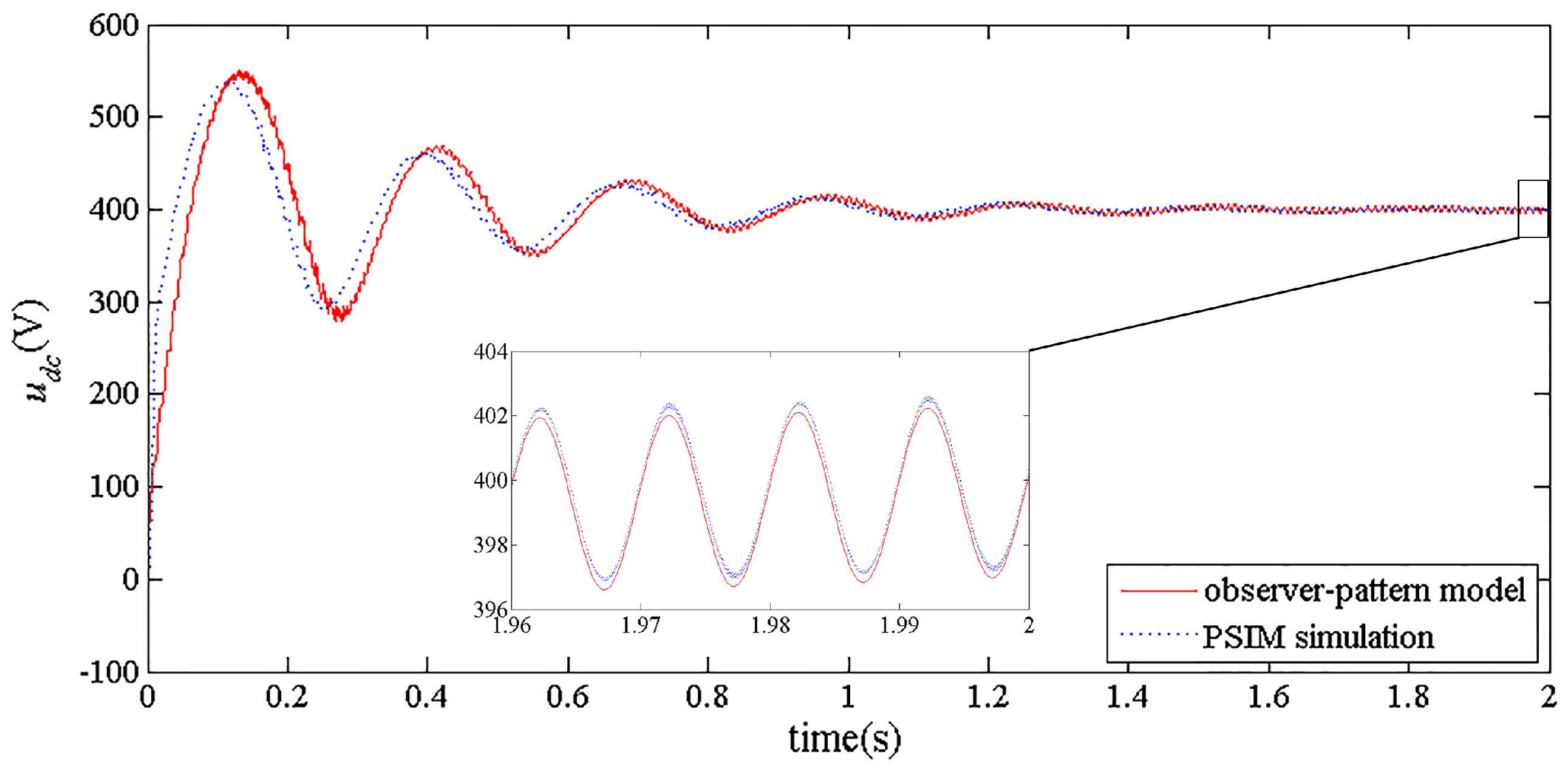
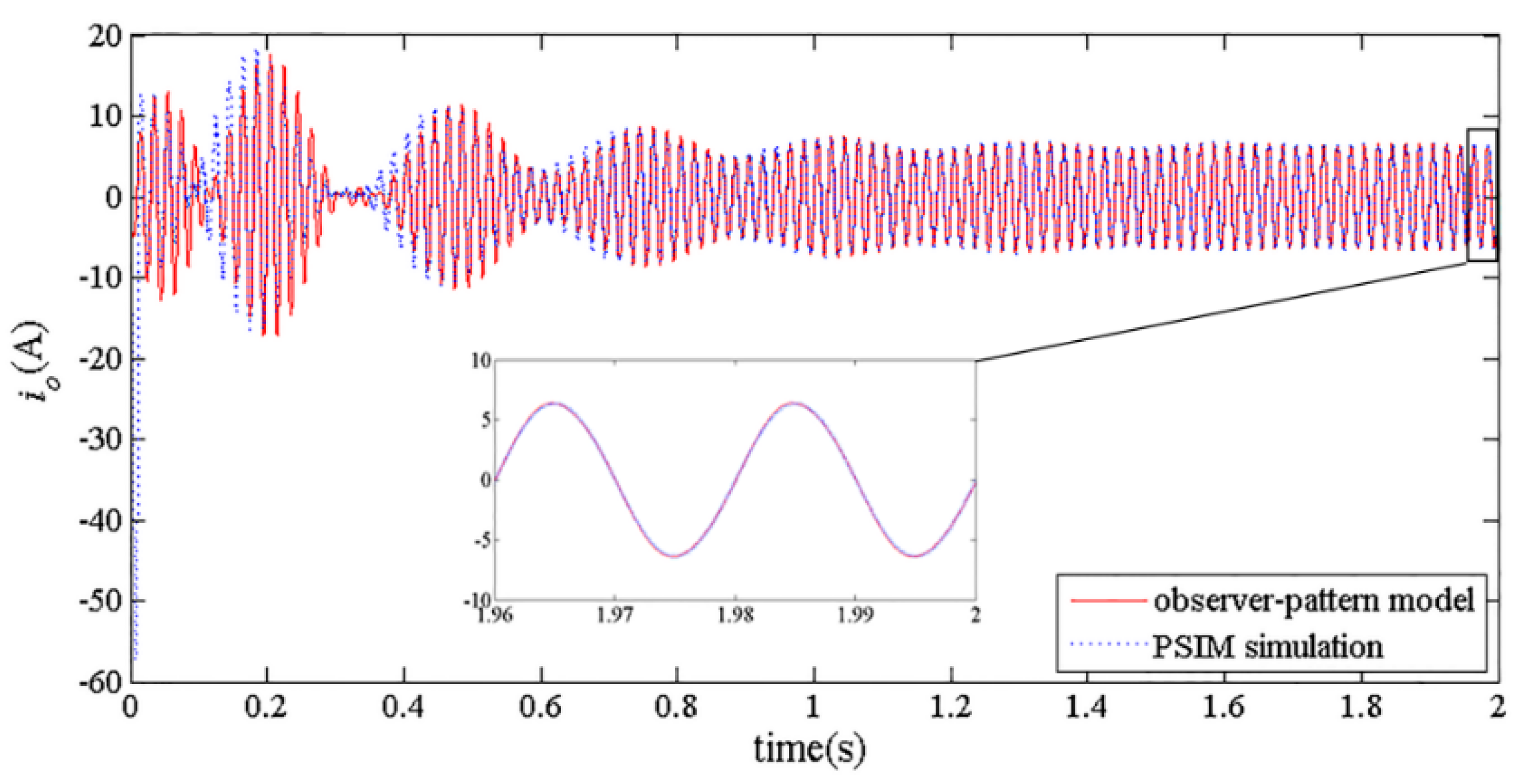
In order to verify the proposed model, simulation results obtained from PSIM are compared to the solutions of the model obtained from MATLAB. The simulation parameters, including PV array parameters and converter parameters, are given in Table 1 and Table 2. Figure 2 and Figure 3 show the simulation waveforms of DC bus voltage udc and output current io, respectively. In both pictures, it can be seen obviously that observer-pattern model and simulation give almost the same results in steady state.
4. Stability Analysis
For simplicity, the observer-pattern model of the system can be written as
where X = [upv, , udc, iod, ioq, uc1, ue, uc2d, uc2q, g1, g2]T. By setting all the differential items in (21) to zero, the equilibrium point Xe = [upve, e, udce, iode, ioqe, uc1e, uee, uc2de, uc2qe, g1e, g2e]T is obtained. Then. the Jacobian A of the observer-pattern model at the equilibrium point can be derived as
Detailed description of Jacobian A is presented in Appendix A.
To analyze the stability of the system, the eigenvalues of Jacobian are used, which can be calculated by
where I is unit matrix.
The gain and the time constant of three PI controllers are key parameters that affect the performance of the system. As these parameters change, the eigenvalues of the system also change. For the purpose of estimating the direction and size of the eigenvalue movement due to variations in system parameters, a sensitivity analysis is often used [28,29]. The eigenvalue sensitivity of λi with respect to an uncertain parameter μ can be calculated as follow:
where ωi and υi are the left and right eigenvectors corresponding to the eigenvalue λi, respectively. If the real part of ∂λi/∂μ is positive, an increase in the parameter μ causes the eigenvalue λi to move towards right in horizontal direction. The size of the horizontal movement is decided by the magnitude of the real part of ∂λi/∂μ. Similarly, the imaginary part of ∂λi/∂μ is associated with the movement in vertical direction.
Table 3 lists the eigenvalue sensitivities with respect to PI controller parameters calculated by (25). For λ1,2, the most sensitive parameter is Kp3 as the real part of the sensitivity of λ1,2 with respect to Kp3 is the largest. The decrease in Kp3 makes λ1,2 move toward right in the s-plane. For λ3,4, the most sensitive parameters are Ti1 and Kp1. A negative perturbation in Ti1 makes λ3,4 move towards right in the s-plane. In contrast, the decrease in Kp3 makes λ3,4 move to left. For λ5, the most critical parameter is Ti1. The increase in Ti1 leads to λ5 moving towards right-half plane. For λ6,7, the most sensitive parameter is Kp2. When Kp2 decreases, λ6,7 moves towards right in the s-plane. For λ8,9, the most sensitive parameters is Ti3. The increase in Ti3 leads to λ8,9 moving towards right in the s-plane. λ10,11 are insensitive to all these parameters listed in Table 3.
Figure 4 illustrates the loci of the eigenvalues with respect to various PI controller parameters. It is obviously that the eigenvalue loci in Figure 4 match the sensitivity analysis results above. Especially note that in Figure 4b, λ3,4 move across the imaginary axis from the left-half plane to the right-half plane when Ti1 decreases to 0.01, which means the system becomes unstable.
The eigenvalues when Ti1 equals to 0.01 and 0.03 are listed in Table 4 as a comparison. It can be seen clearly that λ10,11, which originated from Equation (20), always equals to ±j628. Therefore, λ10,11 is only associated with the angular frequency of power grid and has no influence on the stability of the system. Actually, λ1,2 and λ8,9 are different when Ti1 varies. However, the slight differences are disregarded in this paper. Neglecting λ10,11, all eigenvalues are in the left half of the s-plane when Ti1 = 0.03, and the system operates in a stable state. However, when Ti1 decreases to 0.01, λ3,4 becomes 26.8 ± j1453, which indicates the system is unstable and a low-frequency oscillation occurs. The frequency of the oscillation can be calculated according to the magnitude of the imaginary part of λ3,4 as follows:
Figure 5 presents the simulation results of udc obtained by PSIM when Ti1 equals to 0.03 and 0.01. In Figure 5a, the waveform of udc is sinusoidal and fluctuates around the nominal value. It can be seen clearly that udc contains a DC component and a ripple at 100 Hz. The ripple at 100 Hz is due to pulsating output power of the single-phase inverter [30]. In Figure 5c, the waveform of udc is non-sinusoidal. It can be seen from Figure 5d that the waveform contains a ripple at 100 Hz and a component at 230.5 Hz, which matches the theoretical analysis given by the observer-pattern model.
5. Conclusions
Modeling and stability analysis of a single-phase two-stage grid-connected photovoltaic system have been presented in this paper. (1) An integrated mathematical model including both DC-DC converter and DC-AC converter is developed to capture the dynamics of the system, also the nonlinear characteristic of the PV array is considered in the model; (2) An observer-pattern modeling method is applied to transform the system into time-invariant; (3) Critical controller parameters that influence the stability of the system are identified using eigenvalue sensitivity and eigenvalue loci plots. It is found that Ti1 is closely related to λ3,4. The decrease in Ti1 makes λ3,4 move to left in the s-plane and is disadvantageous to the stability of the system. The theoretical results have been validated by PSIM simulations.
Acknowledgments
This project was supported by the National Natural Science Foundation of China (Grant Nos. 51507068 and 51277079) and the Team Program of Natural Science Foundation of Guangdong Province, China (Grant No. 2017B030312001).
Author Contributions
Liying Huang established the model, implemented the simulation and wrote this article; Dongyuan Qiu guided and revised the paper; Dongyuan Qiu, Fan Xie, Yanfeng Chen, and Bo Zhang guided the research.
Conflicts of Interest
The authors declare no conflict of interest.
Appendix A
The Jacobian matrix A is given as:
where , , , , , , , , , , , , , , , , , , , , , , , , , , , , , , , , , , , , , , , , , , , , , , .
References
- Cucchiella, F.; D’Adamo, I.; Gastaldi, M. Economic analysis of a photovoltaic system: A resource for residential households. Energies 2017, 10, 814. [Google Scholar] [CrossRef]
- Kouro, S.; Leon, J.I.; Vinnikov, D.; Franquelo, L.G. Grid-Connected Photovoltaic Systems: An Overview of Recent Research and Emerging PV Converter Technology. IEEE Ind. Electron. Mag. 2015, 9, 47–61. [Google Scholar] [CrossRef]
- Schimpf, F.; Norum, L. Effective use of film capacitors in single-phase PV-inverters by active power decoupling. In Proceedings of the 36th Annual Conference on IEEE Industrial Electronics Society, Glendale, AZ, USA, 7–10 November 2010; pp. 2784–2789. [Google Scholar]
- Nižetić, S.; Papadopoulos, A.M.; Tina, G.M.; Rosa-Clot, M. Hybrid energy scenarios for residential applications based on the heat pump split air-conditioning units for operation in the Mediterranean climate conditions. Energy Build. 2017, 140, 110–120. [Google Scholar] [CrossRef]
- Xiong, X.; Chi, K.T.; Ruan, X. Bifurcation Analysis of Standalone Photovoltaic-Battery Hybrid Power System. IEEE Trans. Circuits Syst. I Regul. Pap. 2013, 60, 1354–1365. [Google Scholar] [CrossRef]
- Deivasundari, P.; Uma, G.; Poovizhi, R. Analysis and experimental verification of Hopf bifurcation in a solar photovoltaic powered hysteresis current-controlled cascaded-boost converter. IET Power Electron. 2013, 6, 763–773. [Google Scholar] [CrossRef]
- Zhioua, M.; Aroudi, A.E.; Belghith, S.; Bosquemoncusí, J.M.; Giral, R.; Hosani, K.A.; Alnumay, M. Modeling, Dynamics, Bifurcation Behavior and Stability Analysis of a DC–DC Boost Converter in Photovoltaic Systems. Int. J. Bifurc. Chaos 2016, 26, 1650166. [Google Scholar] [CrossRef]
- Al-Hindawi, M.M.; Abusorrah, A.; Al-Turki, Y.; Giaouris, D.; Mandal, K.; Banerjee, S. Nonlinear Dynamics and Bifurcation Analysis of a Boost Converter for Battery Charging in Photovoltaic Applications. Int. J. Bifurc. Chaos 2014, 24, 373–491. [Google Scholar] [CrossRef]
- Abusorrah, A.; Al-Hindawi, M.M.; Al-Turki, Y.; Mandal, K.; Giaouris, D.; Banerjee, S.; Voutetakis, S.; Papadopoulou, S. Stability of a boost converter fed from photovoltaic source. Sol. Energy 2013, 98, 458–471. [Google Scholar] [CrossRef]
- Li, X.; Tang, C.; Dai, X.; Hu, A.; Nguang, S. Bifurcation Phenomena Studies of a Voltage Controlled Buck-Inverter Cascade System. Energies 2017, 10, 708. [Google Scholar] [CrossRef]
- Tse, C.K.; Bernardo, M.D. Complex behavior in switching power converters. Proc. IEEE 2002, 90, 768–781. [Google Scholar] [CrossRef]
- Banerjee, S.; Chakrabarty, K. Nonlinear modeling and bifurcations in the boost converter. IEEE Trans. Power Electron. 1998, 13, 252–260. [Google Scholar] [CrossRef]
- Deane, J.H.B.; Hamill, D.C. Instability, subharmonics, and chaos in power electronic systems. IEEE Trans. Power Electron. 1989, 5, 260–268. [Google Scholar] [CrossRef]
- Aroudi, A.E.; Giaouris, D.; Mandal, K.; Banerjee, S. Complex non-linear phenomena and stability analysis of interconnected power converters used in distributed power systems. IET Power Electron. 2016, 9, 855–863. [Google Scholar] [CrossRef]
- Saublet, L.M.; Gavagsaz-Ghoachani, R.; Martin, J.P.; Nahid-Mobarakeh, B.; Pierfederici, S. Asymptotic Stability Analysis of the Limit Cycle of a Cascaded DC–DC Converter Using Sampled Discrete-Time Modeling. IEEE Trans. Ind. Electron. 2016, 63, 2477–2487. [Google Scholar] [CrossRef]
- Zadeh, M.K.; Gavagsaz-Ghoachani, R.; Pierfederici, S.; Nahid-Mobarakeh, B.; Molinas, M. Stability Analysis and Dynamic Performance Evaluation of a Power Electronics-Based DC Distribution System with Active Stabilizer. IEEE J. Emerg. Sel. Top. Power Electron. 2016, 4, 93–102. [Google Scholar] [CrossRef]
- Xie, F.; Zhang, B.; Qiu, D.; Jiang, Y. Non-linear dynamic behaviours of DC cascaded converters system with multi-load converters. IET Power Electron. 2016, 9, 1093–1102. [Google Scholar] [CrossRef]
- Salis, V.; Costabeber, A.; Cox, S.M.; Zanchetta, P. Stability Assessment of Power-Converter-Based AC Systems by LTP Theory: Eigenvalue Analysis and Harmonic Impedance Estimation. IEEE J. Emerg. Sel. Top. Power Electron. 2017, 5, 1513–1525. [Google Scholar] [CrossRef]
- Cai, H.; Xiang, J.; Wei, W. Modelling, analysis and control design of a two-stage photovoltaic generation system. IET Renew. Power Gener. 2016, 10, 1195–1203. [Google Scholar] [CrossRef]
- Zadeh, M.K.; Gavagsaz-Ghoachani, R.; Nahid-Mobarakeh, B.; Pierfederici, S.; Molinas, M. Stability analysis of hybrid AC/DC power systems for more electric aircraft. In Proceedings of the Applied Power Electronics Conference and Exposition, Long Beach, CA, USA, 20–24 May 2016; pp. 446–452. [Google Scholar]
- Zhang, H.; Wan, X.; Li, W.; Ding, H.; Yi, C. Observer-Pattern Modeling and Slow-Scale Bifurcation Analysis of Two-Stage Boost Inverters. Int. J. Bifurc. Chaos 2017, 27, 1750096. [Google Scholar] [CrossRef]
- Zhang, H.; Li, W.; Ding, H.; Yi, C.; Wan, X. Observer-Pattern Modeling and Nonlinear Modal Analysis of Two-stage Boost Inverter. IEEE Trans. Power Electron. 2017. [Google Scholar] [CrossRef]
- Ram, J.P.; Babu, T.S.; Rajasekar, N. A comprehensive review on solar PV maximum power point tracking techniques. Renew. Sustain. Energy Rev. 2017, 67, 826–847. [Google Scholar] [CrossRef]
- Fadil, H.E.; Giri, F.; Guerrero, J.M. Grid-connected of photovoltaic module using nonlinear control. In Proceedings of the IEEE International Symposium on Power Electronics for Distributed Generation Systems, Aalborg, Denmark, 25–28 June 2012; pp. 119–124. [Google Scholar]
- Franzitta, V.; Orioli, A.; Gangi, A.D. Assessment of the Usability and Accuracy of the Simplified One-Diode Models for Photovoltaic Modules. Energies 2016, 9, 1019. [Google Scholar] [CrossRef]
- Khouzam, K.; Ly, C.; Chen, K.K.; Ng, P.Y. Simulation and real-time modelling of space photovoltaic systems. In Proceedings of the 1994 IEEE 1st World Conference on Photovoltaic Energy Conversion, Waikoloa, HI, USA, 5–9 December 1994; Volume 2, pp. 2038–2041. [Google Scholar]
- Zhang, R.; Cardinal, M.; Szczesny, P.; Dame, M. A grid simulator with control of single-phase power converters in D-Q rotating frame. In Proceedings of the 2002 IEEE 33rd Annual IEEE Power Electronics Specialists Conference, Cairns, Australia, 23–27 June 2002; Volume 3, pp. 1431–1436. [Google Scholar]
- Gao, F.; Zheng, X.; Bozhko, S.; Hill, C.I.; Asher, G. Modal Analysis of a PMSG-Based DC Electrical Power System in the More Electric Aircraft Using Eigenvalues Sensitivity. IEEE Trans. Transp. Electrification 2015, 1, 65–76. [Google Scholar]
- Yang, L.; Xu, Z.; Østergaard, J.; Dong, Z.Y.; Wong, K.P.; Ma, X. Oscillatory Stability and Eigenvalue Sensitivity Analysis of A DFIG Wind Turbine System. IEEE Trans. Energy Convers. 2011, 26, 328–339. [Google Scholar] [CrossRef] [Green Version]
- Shi, Y.; Liu, B.; Duan, S. Low-Frequency Input Current Ripple Reduction Based on Load Current Feedforward in a Two-Stage Single-Phase Inverter. IEEE Trans. Power Electron. 2016, 31, 7972–7985. [Google Scholar] [CrossRef]
Figure 1.
Diagram of a single-phase two-stage grid-connected photovoltaic system: (a) Power stage circuit; (b) MPPT controller; (c) double loop controller.
Figure 1.
Diagram of a single-phase two-stage grid-connected photovoltaic system: (a) Power stage circuit; (b) MPPT controller; (c) double loop controller.
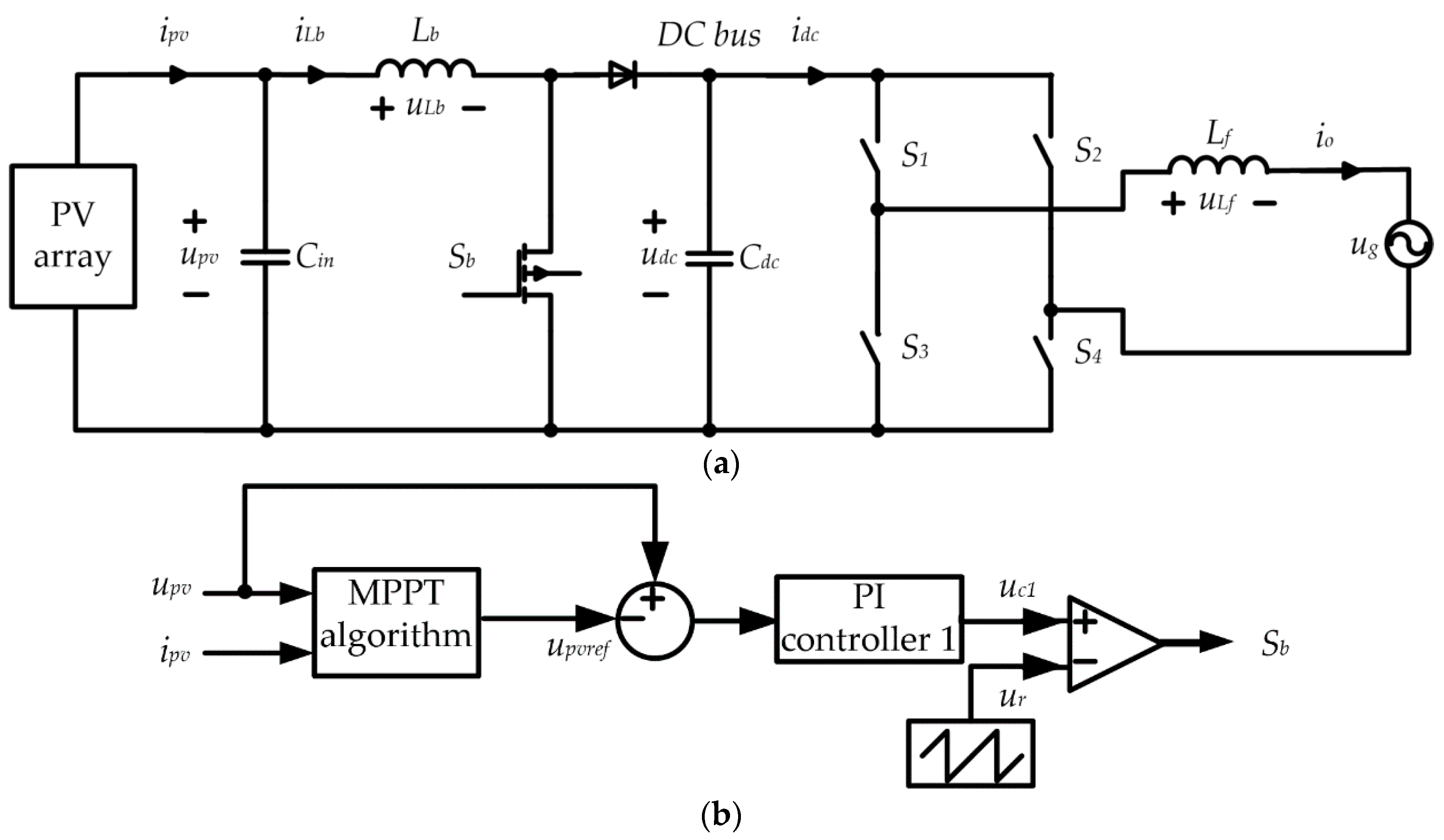

Figure 2.
DC bus voltage waveform.

Figure 3.
Output current waveform.

Figure 4.
Loci of the eigenvalues with respect to various PI controller parameters: (a) λ1,2 when Kp3 is varied within the range (0.2, 1.8); (b) λ3,4 when Ti1 is varied within the range (0.01, 0.19); (c) λ3,4 when Kp1 is varied within the range (0.005, 0.095); (d) λ5 when Ti1 is varied within the range (0.01, 0.19); (e) λ6,7 when Kp2 is varied within the range (0.002, 0.038); (f) λ8,9 when Ti3 is varied within the range (0.02, 0.38).

Figure 5.
Simulation results of udc: (a) Time domain waveforms when Ti1 = 0.03; (b) Fast Fourier Transformation (FFT) analysis when Ti1 = 0.03; (c) Time domain waveforms when Ti1 = 0.01; (d) FFT analysis when Ti1 = 0.01.
Figure 5.
Simulation results of udc: (a) Time domain waveforms when Ti1 = 0.03; (b) Fast Fourier Transformation (FFT) analysis when Ti1 = 0.03; (c) Time domain waveforms when Ti1 = 0.01; (d) FFT analysis when Ti1 = 0.01.


Table 1.
Photovoltaic (PV) array parameters.
| Parameter | Symbol | Quantity |
|---|---|---|
| Voltage at MPP | UM | 119.6 V |
| Current at MPP | IM | 8.36 A |
| Open circuit voltage | UOC | 149.2 V |
| Short circuit current | ISC | 8.81 A |
Table 2.
Converter parameters.
| Parameter | Symbol | Quantity |
|---|---|---|
| Capacitance of input filter | Cin | 1000 μF |
| Inductance of boost converter | Lb | 10 mH |
| Capacitance of boost converter | Cdc | 1500 μF |
| Inductance of output filter | Lf | 25 mH |
| Amplitude of grid voltage | Ugm | 220√2 V |
| Switching frequency | fs | 10 kHz |
| Gain of PI controller 1 | Kp1 | 0.05 |
| Time constant of PI controller 1 | Ti1 | 0.1 |
| Gain of PI controller 2 | Kp2 | 0.02 |
| Time constant of PI controller 2 | Ti2 | 0.01 |
| Gain of PI controller 3 | Kp3 | 1 |
| Time constant of PI controller 3 | Ti3 | 0.2 |
Table 3.
Eigenvalue sensitivities.
| λ1,2 | λ3,4 | λ5 | λ6,7 | λ8,9 | λ10,11 | |
|---|---|---|---|---|---|---|
| Kp1 | −8.93 × 10⁻⁴ ± j7.47 × 10-5 | 5.57 ± j1.38 × 104 | −9.31 | −0.91 ± j0.145 | −2.45 × 10⁻⁵ ± j2.42 × 10-4 | 0 |
| Ti1 | −2.78 × 10⁻⁷ ± j2.88 × 10-8 | −47.5 ± j0.21 | 94.9 | 0.0286 ± j0.193 | 3.85 × 10⁻⁶ ± j3.28 × 10-7 | 0 |
| Kp2 | −937 ± j35.6 | −0.605 ± j0.188 | −0.664 | −134 ± j553 | 0.00347 ± j0.00126 | 0 |
| Ti2 | −11.8 ± j0.68 | −0.0211 ± j0.0846 | 1.47 | 11 ± j1144 | 1.22 × 10⁻⁴ ± j0.00224 | 0 |
| Kp3 | −1.6 × 10⁴ ± j0.977 | 7.45 × 10⁻⁴ ± j0.00145 | −1.35 × 10⁻⁴ | 0.236 ± j0.0336 | 0.00154 ± j0.00409 | 0 |
| Ti3 | −25 ± j7.68 × 10-4 | 2.62 × 10⁻⁵ ± j1.36 × 10-5 | 2.21 × 10⁻⁵ | 0.00141 ± j0.0192 | 25 ± j0.0208 | 0 |
Table 4.
Eigenvalues when Ti1 = 0.01 and Ti1 = 0.03.
| Ti1 | λ1,2 | λ3,4 | λ5 | λ6,7 | λ8,9 | λ10,11 |
|---|---|---|---|---|---|---|
| 0.01 | −16016 ± j314 | 26.8 ± j1453 | −94.7 | −2.947 ± j22.55 | −5 ± j314 | ±j628 |
| 0.03 | −16016 ± j314 | −4.743 ± j1451 | −31.6 | −2.927 ± j22.56 | −5 ± j314 | ±j628 |
© 2017 by the authors. Licensee MDPI, Basel, Switzerland. This article is an open access article distributed under the terms and conditions of the Creative Commons Attribution (CC BY) license (http://creativecommons.org/licenses/by/4.0/).
Share and Cite
MDPI and ACS Style
Huang, L.; Qiu, D.; Xie, F.; Chen, Y.; Zhang, B. Modeling and Stability Analysis of a Single-Phase Two-Stage Grid-Connected Photovoltaic System. Energies 2017, 10, 2176. https://doi.org/10.3390/en10122176
AMA Style
Huang L, Qiu D, Xie F, Chen Y, Zhang B. Modeling and Stability Analysis of a Single-Phase Two-Stage Grid-Connected Photovoltaic System. Energies. 2017; 10(12):2176. https://doi.org/10.3390/en10122176
Chicago/Turabian StyleHuang, Liying, Dongyuan Qiu, Fan Xie, Yanfeng Chen, and Bo Zhang. 2017. "Modeling and Stability Analysis of a Single-Phase Two-Stage Grid-Connected Photovoltaic System" Energies 10, no. 12: 2176. https://doi.org/10.3390/en10122176
Note that from the first issue of 2016, this journal uses article numbers instead of page numbers. See further details here.