Hybrid Chaotic Quantum Bat Algorithm with SVR in Electric Load Forecasting

Abstract

Hybridizing evolutionary algorithms with a support vector regression (SVR) model to conduct the electric load forecasting has demonstrated the superiorities in forecasting accuracy improvements. The recently proposed bat algorithm (BA), compared with classical GA and PSO algorithm, has greater potential in forecasting accuracy improvements. However, the original BA still suffers from the embedded drawbacks, including trapping in local optima and premature convergence. Hence, to continue exploring possible improvements of the original BA and to receive more appropriate parameters of an SVR model, this paper applies quantum computing mechanism to empower each bat to possess quantum behavior, then, employs the chaotic mapping function to execute the global chaotic disturbance process, to enlarge bat’s search space and to make the bat jump out from the local optima when population is over accumulation. This paper presents a novel load forecasting approach, namely SVRCQBA model, by hybridizing the SVR model with the quantum computing mechanism, chaotic mapping function, and BA, to receive higher forecasting accuracy. The numerical results demonstrate that the proposed SVRCQBA model is superior to other alternative models in terms of forecasting accuracy.

1. Introduction

Electric load forecasting plays an essential role in making optimal action plans for decision makers, such as load unit commitment, energy transfer scheduling, contingency planning load shedding, energy generation, load dispatch, power system operation security, hydrothermal coordination, and so on [1]. Indicated by Bunn and Farmer [2], an 1% increase in electric load forecasting error may lead to a £10 million additional expenditure in operations. Thus, it is important to look for high accurate forecasting models or to develop novel approaches to receive satisfied load forecasting accuracy, which can help decision makers optimize adjust the electricity price/supply and load plan based on the forecasted results, i.e., improve the electricity system operations more efficient, and reduce system operating risks successfully. Unfortunately, affected by several exogenous factors, such as policy, economic production, industrial activities, weather conditions, population, holidays, etc. [3], the electric load data demonstrate seasonality, non-linearity, volatility, randomness and chaos in nature, which increase the difficulty for electric demand forecasting [4].

In the past few decades, lots of electric load forecasting models have been developed to improve load forecasting accuracy. These forecasting methods include two classical types: traditional statistical models and artificial intelligent models. The traditional statistical models are easily to be applied, which include the ARIMA model [5], Kalman filtering/linear quadratic estimation model [6], exponential smoothing model [7], regression model [8], Bayesian estimation model [9], and other time series technologies [10]. However, most of the traditional statistical models are theoretically to deal with the linear relationships among electric loads and other factors; these methods are difficult to well handle the characteristics of non-linearity, volatility, and randomness among historical electric loads and exogenous factors. Thus, they cannot easily receive satisfied electric load forecasting accuracy.

Due to the strong nonlinear fitting ability, various artificial intelligence (AI) based methods have been applied to forecast electric load, to improve the accuracy of load forecasting models since 1980s, such as artificial neural networks (ANNs) [11], expert system-based model [12], and fuzzy inference methodology [13]. To further improve the forecasting performance, these AI methods have been hybridized or combined with each other to obtain new novel forecasting approaches or frameworks, for example, RBF neural network combined with adaptive network-based fuzzy inference system [14], multi-layer perceptron artificial neural network hybridized with knowledge-based feedback tuning fuzzy system (MLPANN) [15], the Bayesian neural network with the hybrid Monte Carlo algorithm [16], fuzzy behavior neural network (WFNN) [17], hybrid artificial bee colony algorithm hybridized with extreme learning machine [18], the random fuzzy variables with ANNs [19], and so on. However, these AI-based approaches still suffer from some embedded drawbacks. The defects of these models include difficulty to set the structural parameters of network [20], time consuming to extract functional approximation, and easily to trapped in local optimal value. More systematic analysis about AI-based models used in load forecasting are shown in references [21].

Support vector machine (SVM) is based on the statistical learning theory and kernel computing techniques, the so-called kernel based neural networks, to effectively deal with small sample size problem, non-linear problem, and high dimensional pattern identification problems. Moreover, it could also be applied to well solve other machine learning problems, such as function approximation, probability density estimation, and so on [22,23]. Rather than by implementing the empirical risk minimization (ERM) principle to minimize the training error, which causes the overfitting problem in the ANNs modeling process, SVM employs the structural risk minimization (SRM) principle to minimize an upper bound on the generalization error, and allow learning any training set without error. Thus, SVMs could theoretically guarantee to achieve the global optimum than ANNs models. In addition, while dealing with the nonlinear problem, SVM firstly maps the data into a higher dimensional space, then, it employs the kernel function to replace the complicate inner product in the high dimensional space. In the other words, it can easily avoid too complex computations with high dimensions, i.e., the so-called dimension disaster problem. This enables SVMs to be a feasible choice for solving a variety of problems in lots of fields which are non-linear in nature. For more detailed mechanisms introduction of SVMs, it is referred to Vaplink [22,23] and Scholkopf and Sloma [24], among others. Along with the introduction of Vapnik’s $\epsilon$-insensitive loss function, SVM also has been extended to solve nonlinear regression estimation problems, which are so-called support vector regression (SVR) [25]. Compared with AI methods, SVR model has the embedded characteristics of small sample learning and generalization ability, which can avoid learning, local minimal point and dimension disaster problem effectively. SVR have been successfully employed to solve forecasting problems in many fields, such as solar irradiation forecasting [26], rainfall/flood hydrological forecasting [27,28,29], industrial wastewater quality forecasting [30], and so on. Meanwhile, SVR model had also been successfully applied to forecast electric load [31,32]. To improve the forecasting accuracy, Hong and his colleagues propose a series of SVR-based forecasting models via hybridizing with different evolutionary algorithms [33,34,35,36]. Based on Hong’s series research results, well determining parameters of an SVR model is critical to improve the forecasting performance. Henceforth, Hong and his successors have employed chaotic mapping functions (including logistic function and cat mapping function) to enrich diversity of population over the whole space, and also have applied cloud theory to execute the three parameters selection carefully to receive significant improvements in terms of forecasting accuracy.

Bat algorithm [37] is a new swarm intelligent optimization proposed by Yang in 2010. It is originated from the simulation of bat’s prey detection and obstacle avoidance by sonar. This algorithm is a simulation technology based on iteration. The population is initialized randomly, then the optimal resolution is searched through iteration, finally the local new resolutions are found around the optimal resolution by random flying, hence, the local search is strengthened. Compared with other algorithms, BA has the advantages of parallelism, quick convergence, distribution and less parameter adjusted. It has been proved that BA is superior to PSO in terms of convergent rate and stability [38]. Nowadays, BA is widely applied in natural science, such as PFSP dispatch problem [39], K-means clustering optimization [40], engineering optimization [41], and multi-objective optimization [42], etc. Comparing with other evolutionary algorithms, such as, PSO and GA, BA has greater improving potential. However, similar to those optimization algorithms which are based on population iterative searching mechanism, standard BA also suffers from slow convergent rate in the later searching period, weak local search ability and premature convergence tendency [41].

On the other hand, quantum computing technique is an important research hotspot in the field of intelligent computing. The principle of qubit and superposition of states in quantum computing is used. The units are represented by qubit coding, and the revolution is updated by quantum gate, which expands its ergodic ability in solution space. Recently, it has received some hot attention that quantum computing concepts could be theoretically hybridized with those evolutionary algorithms to improve their searching performances. Huang [43] proposes an SVR-based forecasting model by hybridizing the quantum computing concepts and the cat mapping function with the PSO algorithm into an SVR model, namely SVRCQPSO forecasting model, and receives satisfied forecasting accurate levels. Lee and Lin [44,45] also hybridize the quantum computing concepts and cat mapping function with tabu search algorithm and genetic algorithm to propose SVRCQTS and SVRCQGA models, respectively, and also receive higher forecasting accuracy. Li et al. [46] also applied quantum non-gate to realize quantum mutation to avoid premature convergence. Their experiments on classical complicated functions also reveal that the improved algorithm could effectively avoid local optimal solutions. However, due to the population diversity decline along with iterative time increasing, the BA and QBA still suffers from the very problem that trapping into local optima and premature convergence.

Considering the core drawback of the BA and QBA, i.e., trapping into local optima, causing unsatisfied forecasting accuracy, this paper would continue to explore the feasibility of hybridizing quantum computing concepts with BA, to overcome the premature problem of BA, eventually, to determine more suitable parameter combination of an SVR model. Therefore, this paper employs quantum computing concepts to empower each bat to expand the search space during the searching processes of BA; in the meanwhile, also applies the chaotic mapping function to execute global perturbation operation to help the bats jump from the local optima when the diversity of the population is poor; then, receive more suitable parameter combination of an SVR model. Finally, a new load forecasting model, via hybridizing cat mapping function, quantum computing concepts and BA with an SVR model, namely SVRCQBA model, is proposed. Furthermore, the forecasting results of SVRCQBA model are used to compare with that of other alternatives proposed by Huang [43] and Lee and Lin [44,45] to test its superiority in terms of forecasting accuracy. The main innovative contribution of this paper is continuing to hybridize the SVR model with the quantum computing mechanism, chaotic mapping theory and evolutionary algorithms, to well explore the load forecasting model with higher accurate levels.

The remainder of this article is organized as follows. The basic formulation of an SVR model, the proposed CQBA and the implementation details of the proposed SVRCQBA model are illustrated in Section 2. Section 3 presents a numerical example and achieves the compared analysis among the proposed model and published alternative models. Finally, Section 4 concludes this paper.

2. Methodology of SVRCQBA Model

2.1. Support Vector Regression (SVR) Model

The brief ideas of SVR are demonstrated. A non-linear mapping function, $\phi \left(x\right)$, is defined to map the input data set, ${\left\{\left(x_i,y_i\right)\right\}}_{i=1}^N$, into a high dimensional feature space. Then, there theoretically exists a linear function, f, to formulate the non-linear relationships between input data and output data. The linear function, f, is the so-called the SVR function, and is shown as Equation (1),

$$f\left(x\right)=w^T\phi \left(x\right)+b$$

(1)

where $f\left(x\right)$ represents the forecasting values; $\phi \left(x\right)$ is the feature mapping function, non-linearly mapping the input space, x, into the feature space; the coefficients, w and b, are determined by minimizing the empirical risk, as shown in Equation (2),

$$R_{emp}\left(f\right)=\frac{1}{N}{\displaystyle \sum }_{i=1}^N{L}_{\epsilon }(y_i,w^T\phi \left(x_i\right)+b)$$

(2)

where $L_{\epsilon }\left(y, f\left(x\right)\right)$ is the $\epsilon$-insensitive loss function as shown in Equation (3),

$$L_{\epsilon }\left(y,f\left(x\right)\right)=\{\begin{array}{cc}\left|f\left(x\right)-y\right|-\epsilon & if \left|f\left(x\right)-y\right|\ge \epsilon \\ 0& otherwise\end{array}$$

(3)

In addition, $L_{\epsilon }\left(y, f\left(x\right)\right)$ is used to look for an optimum hyper plane in the feature space, to maximize the distance separating the training data into two subsets. Thus, the SVR focuses on looking for the optimum hyper plane, and minimizing the training errors between the training data and the $\epsilon$-insensitive loss function.

Therefore, the SVR modeling problem could be illustrated as minimizing the overall errors, shown in Equation (4),

$$\underset{w,b,{\xi }^{*},\xi }{\min } R_{\epsilon }\left(w,{\xi }^{*},\xi \right)=\frac{1}{2}{w}^{T}w+C{\displaystyle \sum }_{i=1}^N\left({\xi }_i^{*}+{\xi }_i\right)$$

(4)

with the constraints,

$$\begin{array}{c}{y}_i-w^T\phi \left(x_i\right)-b\le \epsilon +{\xi }_i^{*},\\ -y_i-w^T\phi \left(x_i\right)-b\le \epsilon +{\xi }_i,\\ {\xi }_i^{*}\ge 0\\ {\xi }_i\ge 0\\ i=1, 2,\dots , N\end{array}$$

The first term of Equation (4), representing the concept that maximizes the distance within two separated training data, is used to penalize large weights, in the meanwhile, to maintain the flatness of $f\left(x\right)$. The second term penalizes training errors via the $\epsilon$-insensitive loss function. C is a parameter to trade off of $f\left(x\right)$ and y. Training errors under $\epsilon$ are denoted as ${\xi }_i^{*}$, whereas training errors above $\epsilon$ are denoted as ${\xi }_i$.

After solving the quadratic optimization problem with inequality constraints, the parameter vector w in Equation (1) is computed as Equation (5),

$$w={\displaystyle \sum }_{i=1}^N\left({\alpha }_i^{*}-{\alpha }_i\right)\phi \left(x_i\right)$$

(5)

where ${\alpha }_i^{*}$, ${\alpha }_i$ are computed and named as Lagrangian multipliers. Finally, the SVR regression function is obtained as Equation (6) in the dual space,

$$f\left(x\right)={\displaystyle \sum }_{i=1}^N\left({\alpha }_i^{*}-{\alpha }_i\right)K\left(x_i,x\right)+b$$

(6)

where $K\left(x_i,x_j\right)$ is the so-called kernel function, and its value could be calculated via the inner product of two vectors, $x_i$ and $x_j$, in the feature space, $\phi \left(x_i\right)$ and $\phi \left(x_j\right)$, respectively, i.e., $K\left(x_i,x_j\right)=\phi \left(x_i\right)·\phi \left(x_j\right)$. Any function that satisfies Mercer’s condition [25] could be used as the kernel function.

The most famous kernel functions are the Gaussian RBF with a width of $\sigma$, and the polynomial kernel with an order of d and constants a₁ and a₂, as shown in Equations (7) and (8), respectively. If the value of $\sigma$ is large enough, the RBF kernel function would approximate to the linear kernel (i.e., polynomial with an order of 1). In addition, the Gaussian RBF kernel function is not only easier to implement, but also capable to non-linearly map the data into the higher dimensional space, thus, it is suitable to deal with non-linear problems. Therefore, the Gaussian RBF kernel function (Equation (7)) is used in this paper.

$$K\left(x_i,x_j\right)=e^{-\frac{{||x}_i-x_j{||}^2}{2{\sigma }^2}}$$

(7)

$$K\left(x_i,x_j\right)={\left(a_1{x}_i{x}_j+a_2\right)}^d$$

(8)

The selection of the three parameters, σ, C, and ε of an SVR model influence the accuracy of forecasting. For parameter, ε, it represents the parameter of the $\epsilon$-insensitive loss function. It controls the width of insensitive area (i.e., low noise of the data set) from data set, thus, it determines the amount of support vectors. If ε is too large, the amount of support vectors would be few, thus, the forecasting model would become relative simple and with low accuracy; on the contrary, if ε is very small, the regression accuracy could be enhanced, however, the forecasting model would become relatively complicate and with low general adoptions.

For parameter, C, it represents the penalty for those data outside the ε-tube. It determines the complexity and stability of the forecasting model. If C is very small, the penalty is mall, i.e., the training errors are large; on the contrary, if C is too large, the learning accuracy would also be enhanced, however, the forecasting model would be with low general adoptions. In addition, the values of C would also affect the fatness of the forecasting model, i.e., the arrangements of outliers. For a suitable C, it could deal with the disturbance of these outliers, and hence, it could guarantee the stability of the forecasting model. Therefore, the suitable parameter determination of C and ε, it could receive more accurate and more stable forecasting model.

For parameter, σ, it not only represents the basic capability of the Gaussian RBF kernel function to deal with nonlinear relationships among data, but also reflects the correlations among support vectors. For example, if σ is very small, the correlation among those support vectors is weak, then, the process of machine learning is relatively complex, i.e., it cannot guarantee to receive general adoptions; on the contrary, if σ is too large, the correlation among those support vectors is too strong to receive sufficient accuracy. Therefore, in the modeling processes, if σ is approximating smaller, it is suggested set a larger value of C.

Based on the above analysis of these three parameters, the complexity and general adoptions of an SVR model are determined by these three parameters and their interactions. Therefore, too look for a novel algorithm to optimize the parameter combination is an important issue to improve the forecasting accuracy of an SVR model.

2.2. Chaotic Quantum Bat Algorithm (CQBA)

2.2.1. Bat Algorithm (BA)

Bats detect preys and avoid obstacles with sonar. According to echolocation in acoustic theory, bats judge preys’ size through adjusting phonation frequency. By the variation of echolocation, bats would detect the distance, direction, velocity, size, etc. of objects, which guarantees bats’ accurate flying and hunting [47]. While searching for preys, they change the volume, A(i), and emission velocity, R(i), of impulse automatically. During the prey-searching period, the ultrasonic volume that they send out is high, while the emission velocity is relatively low. Once the prey is locked, the impulse volume turns down and emission velocity increases with the distance between bat and prey being shortened.

The bat algorithm is a meta heuristic algorithm for intelligent search. The theory is as followings, (1) Bat’s position and velocity are initialized, and are treated as the solution in problem space; (2) The optimal fitness function value of the problem is calculated; (3) The volume and velocity of bat units are adjusted, and are transformed towards optimal unit; (4) The optimal solution is finally received. The bat algorithm involves global search and local search.

In global search, suppose that the search space is with d dimensions, at the time, t, the ith bat has its position, $x_i^t$, and velocity, $v_i^t$. At the time, t + 1, its position, $x_i^{t+1}$, and velocity, $v_i^{t+1}$, are updated as Equations (9) and (10), respectively,

$$x_i^{t+1}=x_i^t+v_i^{t+1}$$

(9)

$$v_i^{t+1}=v_i^t+\left(x_i^t-x_{*}\right)F_i$$

(10)

where $x_{*}$ is the current global optimal solution; $F_i$ is the sonic wave frequency, as shown in Equation (11),

$$F_i=F_{\min }+\left(F_{\max }-F_{\min }\right)\beta$$

(11)

where $\beta \in \left[0,1\right]$ is a random number; $F_{\max }$ and $F_{\min }$ are respectively the sonic wave max frequency and min frequency of the ith bat at this moment. In the process of practice, according to the scope that this problem needs to search, the initialization of each bat is assigned one random frequency following uniform distribution in $\left[F_{\min },F_{\max }\right]$.

In local search, once a solution is selected in the current global optimal solution, each bat would produce new alternative solution in the mode of random walk according to Equation (12),

$$x_{\mathrm{new}}\left(i\right)=x_{\mathrm{old}}+\lambda A^t$$

(12)

where $x_{\mathrm{old}}$ is a solution randomly chosen in current optimal disaggregation; $A^t$ is the average of volume in current bat population; $\lambda$ is a D dimensional vector in [−1, 1].

The bat’s velocity and position update steps are similar to that in standard PSO. In PSO, $F_i$ actually dominates the moving range and space of the particle swarm. To a certain degree, BA could be treated as the balance and combination between standard PSO and augmented local search. The balance is dominated by impulse volume, A(i), and impulse emission rate, R(i). When the bat locks the prey, the volume, A(i), is reduced and the emission rate, R(i), is increased. The impulse volume, A(i), and impulse emission rate, R(i), are updated as Equations (13) and (14), respectively,

$$A^{t+1}\left(i\right)=\gamma A^t\left(i\right)$$

(13)

$$R^{t+1}\left(i\right)=R^0\left(i\right)\left[1-e^{-\delta t}\right]$$

(14)

where, $0<\mathsf{\gamma }<1$, $\delta >0$, are both constants. It is obviously that as $t\to \infty$, then, $A^t\left(i\right)\to 0$ and $R^t\left(i\right)=R^0\left(i\right)$. In the practice process, $\gamma =\delta =0.95$.

2.2.2. Quantum Computing for BA

a.  Quantum Bat Population Initialization

In quantum bat algorithm, the probability amplitude of qubit is applied as the code of bat in current position. Considering the randomness of code in population initialization, the coding program of the bat $B^i$ in this paper is given as Equation (15),

$$B^i=\left[\begin{array}{cccccc}\cos {\theta }_1^i& \cos {\theta }_2^i& \cdots & \cos {\theta }_j^i& \cdots & \cos {\theta }_d^i\\ \sin {\theta }_1^i& \sin {\theta }_2^i& \cdots & \sin {\theta }_j^i& \cdots & \sin {\theta }_d^i\end{array}\right]$$

(15)

where, ${\theta }_j^i=2\pi \times rand\left(·\right)$, $rand\left(·\right)$ is the random number in (0,1); $i=1, 2,\dots ,N$; j = 1, 2,…, d; d is the space dimensionality.

Thus, it can be seen that each bat occupies 2 positions in the ergodic space. The probability amplitudes of each corresponding to the quantum state of $|0⟩$ and $|1⟩$ are defined as Equations (16) and (17), respectively. For convenience, $B_c^i$ is called cosinusoidal position, $B_s^i$ is called sinusoidal position.

$$B_c^i=\left(\cos {\theta }_1^i,\cos {\theta }_2^i,\dots ,\cos {\theta }_j^i,\dots ,\cos {\theta }_d^i\right)$$

(16)

$$B_s^i=\left(\sin {\theta }_1^i,\sin {\theta }_2^i,\dots ,\sin {\theta }_j^i,\dots ,\sin {\theta }_d^i\right)$$

(17)

b.  Quantum Bat Global Search and Local Search

In QBA, the move of bat’s position is actualized by quantum revolving gate. Thus, in standard BA, the update of bat’s moving velocity transforms into the update of quantum revolving gate, the update of bat’s position transforms into the update of bat’s qubit probability amplitude. The optimal positions of the current population are set as Equations (18) (for quantum state of $|0⟩$) and (19) (for quantum state of $|1⟩$), respectively,

$$B_c^g=\left(\cos {\theta }_1^g,\cos {\theta }_2^g,\dots ,\cos {\theta }_d^g\right)$$

(18)

$$B_s^g=\left(\sin {\theta }_1^g,\sin {\theta }_2^g,\dots ,\sin {\theta }_d^g\right)$$

(19)

Based on the assumption above, the update rule of bats’ state is as followings.

In global search, the update rule of the qubit probability amplitude increment of bat $B^i$ is as Equation (20),

$$∆{\theta }_j^i\left(t+1\right)=∆{\theta }_j^i\left(t\right)+F_i∆{\theta }_g$$

(20)

where $∆{\theta }_g$ is defined as Equation (21),

$$∆{\theta }_g=\{\begin{array}{cc}2\pi +{\theta }_j^g-{\theta }_j^i,& {\theta }_j^g-{\theta }_j^i<-\mathsf{\pi }\\ {\theta }_j^g-{\theta }_j^i,& -\pi \le {\theta }_j^g-{\theta }_j^i\le \mathsf{\pi }\\ {\theta }_j^g-{\theta }_j^i-2\pi ,& {\theta }_j^g-{\theta }_j^i>\mathsf{\pi }\end{array}$$

(21)

In local search, the update rule of the qubit probability amplitude corresponding to the current optimal phase increment of bat $B^i$ is defined as Equation (22),

$$∆{\theta }_j^i\left(t+1\right)=e^{-\frac{\omega ·gen}{gen\_max}·average\left(A\right)·\rho }$$

(22)

where, ω is constant; gen is the current iteration number; gen_max is the maximal iteration number; average(A) is the average of current amplitude of each bat; $\rho$ is the random integer in [−1, 1].

c.  Quantum bat location updating

Based on quantum revolving gate, the quantum probability amplitude is updated as Equation (23),

$$\left[\begin{array}{c}\cos \left({\theta }_j^i\left(t+1\right)\right)\\ \sin \left({\theta }_j^i\left(t+1\right)\right)\end{array}\right]=\left[\begin{array}{cc}\cos \left(∆{\theta }_j^i\left(t+1\right)\right)& -\sin \left(∆{\theta }_j^i\left(t+1\right)\right)\\ \sin \left(∆{\theta }_j^i\left(t+1\right)\right)& \cos \left(∆{\theta }_j^i\left(t+1\right)\right)\end{array}\right]\times \left[\begin{array}{c}\cos \left({\theta }_j^i\left(t\right)\right)\\ \sin \left({\theta }_j^i\left(t\right)\right)\end{array}\right]=\left[\begin{array}{c}\cos \left({\theta }_j^i\left(t\right)+∆{\theta }_j^i\left(t+1\right)\right)\\ \sin \left({\theta }_j^i\left(t\right)+∆{\theta }_j^i\left(t+1\right)\right)\end{array}\right]$$

(23)

The two new updated positions (for the quantum state of $|0⟩$ and $|1⟩$) of bat $B^i$ are shown as Equations (24) and (25), respectively,

$$P_c^i\left(t+1\right)=\left(\cos ({\theta }_1^i\left(t\right)+∆{\theta }_1^i\left(t+1\right)),\dots ,\cos \left({\theta }_d^i\left(t\right)+∆{\theta }_d^i\left(t+1\right)\right)\right)$$

(24)

$$P_s^i\left(t+1\right)=\left(\sin ({\theta }_1^i\left(t\right)+∆{\theta }_1^i\left(t+1\right)),\dots ,\sin \left({\theta }_d^i\left(t\right)+∆{\theta }_d^i\left(t+1\right)\right)\right)$$

(25)

It demonstrates that quantum revolving gate actualizes the simultaneous movements of bat’s two positions by updating qubit phase which depicts the bat’s position. Thus, under the condition of unchanging total population size, the qubit encoding can enhance ergodicity, which helps improving the efficiency of the algorithm.

2.2.3. Chaotic Quantum Global Perturbation

As a bionic evolutionary algorithm, with the increasing number of iterations, the diversity of the population will decline, which leads to premature convergence during optimization processes. As mentioned, the chaotic variable can be used to maintain diversity of the population to avoid premature convergence. Many scholars have published papers using improved chaotic algorithm [48,49]. Authors also have used cat map to the improve GA and PSO algorithm [50,51], the results of numerical experiments show that the searching ability of new GA and PSO improved by chaos is enhanced. Hence, in this paper, the cat mapping function is employed to be the global chaotic perturbation strategy (GCPS), i.e., the so-called CQBA, based on the QBA to adopt GCPS while suffering from premature convergence problem in the iterative searching processes.

The two-dimensional cat mapping function is shown as Equation (26),

$$\{\begin{array}{c}{y}^{t+1}=frac\left(y^t+z^t\right)\\ z^{t+1}=frac\left(y^t+2z^t\right)\end{array}$$

(26)

where frac function is employed for the fractional parts of a real number y by subtracting an appropriate integer.

The global chaotic perturbation strategy (GCPS) is illustrated as followings.

(1)

Generate $\frac{\mathit{N}}{\mathit{2}}$ chaotic disturbance bats. For each $Ba{t}^i$(i = 1, 2, …, N), apply Equation (26) to generate d random numbers, $z_j$ (j = 1, 2, …, d). Then, the Equations (27) and (28) are used to map these numbers, $z_j$, into $y_j$ (with valued from −1 to 1). Set $y_j$ as the qubit (with quantum state, $|0⟩$) amplitude, $\cos {\theta }_j^i$, of $Ba{t}^i$.

$$\frac{z_j-0}{1-0}=\frac{y_j-\left(-1\right)}{1-\left(-1\right)}$$

(27)

$$\cos {\theta }_j^i=y_j=2z_j-1$$

(28)

(2)

Determine the $\frac{\mathit{N}}{\mathit{2}}$ bats with better fitness. Calculate fitness value of each bat from current QBA, and arrange these bats to be a sequence in the order of fitness values. Then, select the bats with the $\frac{N}{2}$th ranking ahead in the fitness values.

(3)

Form the new CQBA population. Mix the $\frac{N}{2}$ chaotic perturbation bats with the $\frac{N}{2}$ bats which are with better fitness selected from current QBA, and form a new population that contains new N bats, and named it as CQBA population.

(4)

Complete global chaotic perturbation. After obtaining the new CQBA population, take the new CQBA population as the new population of QBA, and continue to execute the QBA process.

2.2.4. Implementation Steps of CQBA

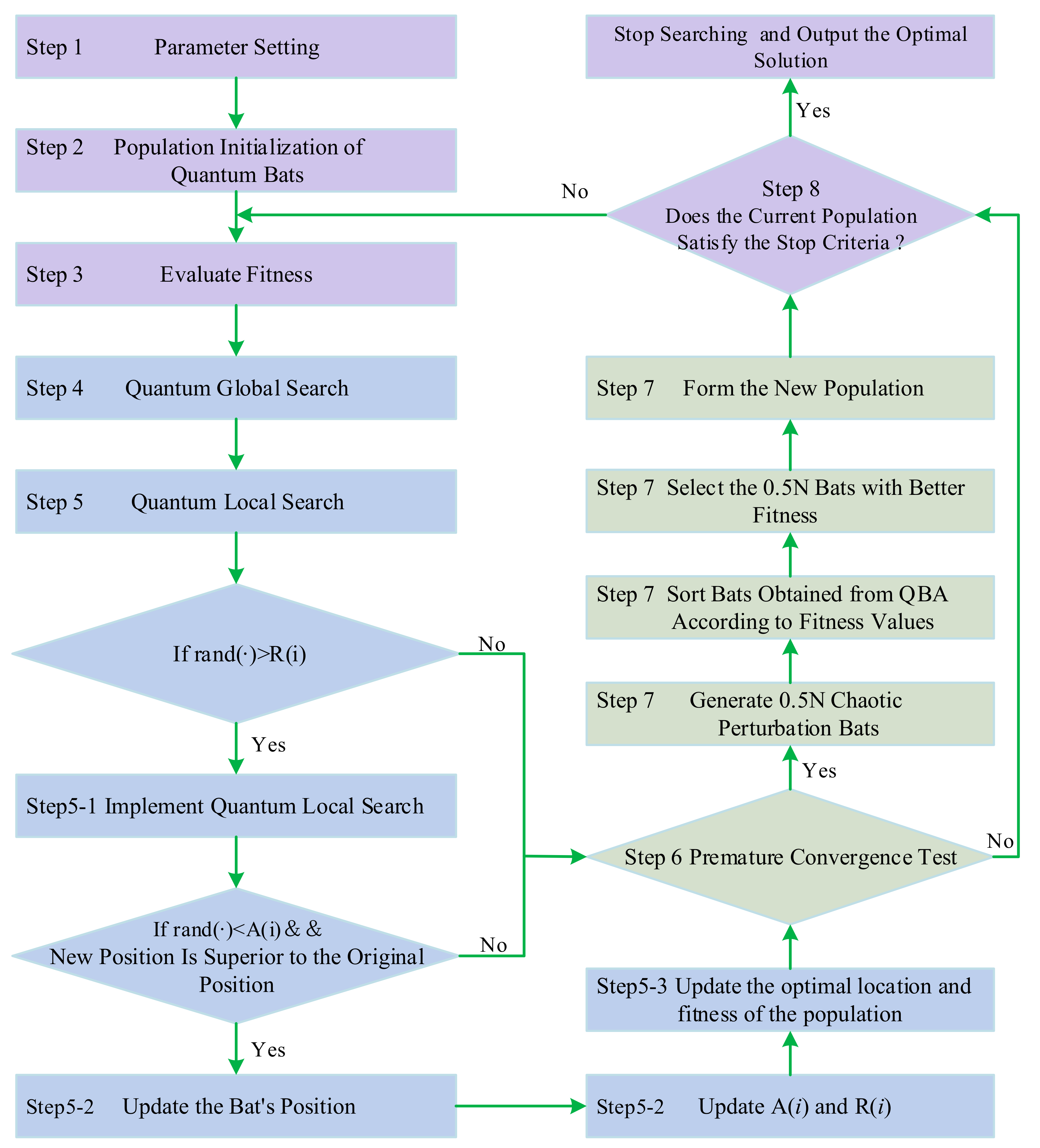
The procedure of the hybrid CQBA with an SVR model is detailed as followings and the associate flowchart is provided as Figure 1.

Step 1

Parameter Setting. Initialize the population size, N; maximal iteration, gen_max; expected criteria, $\vartheta$; pulse emission rate, R(i); maximum and minimum of emission frequencies, $F_{\max }$ and $F_{\min }$, respectively.

Step 2

Population Initialization of Quantum Bats. According to quantum bat population initialization strategy, initialize quantum bat population randomly.

Step 3

Evaluate Fitness. Evaluate the objective fitness by employing the coding information of quantum bats. Each probability amplitude of qubit is corresponding to an optimization variable in solution space. Assumed that the jth qubit of the bat $B^i$ is $\left[\begin{array}{c}{\eta }_j^i\\ {\zeta }_j^i\end{array}\right]$, the element’s value of the qubit is between the interval, [−1, 1]; the solution space variable corresponding to that is $\left[\begin{array}{c}{\left(X_j^i\right)}_c\\ {(X_j^i)}_s\end{array}\right]$, set the element’s value be between the interval, [a_j, b_j]. Then, the solution could be calculated by the equal proportion relationship (i.e., Equations (29) and (30)),

$$\frac{{(X_j^i)}_c-a_j}{b_j-a_j}=\frac{{\eta }_j^i-\left(-1\right)}{1-\left(-1\right)}$$

(29)

$$\frac{{(X_j^i)}_s-a_j}{b_j-a_j}=\frac{{\zeta }_j^i-\left(-1\right)}{1-\left(-1\right)}$$

(30)

Eventually, the solution $\left[\begin{array}{c}{\left(X_j^i\right)}_c\\ {(X_j^i)}_s\end{array}\right]$ is obtained as shown in Equations (31) and (32).

$${(X_j^i)}_c=\frac{1}{2}\left[b_j\left(1+{\eta }_j^i\right)+a_j\left(1-{\eta }_j^i\right)\right]$$

(31)

$${(X_j^i)}_s=\frac{1}{2}\left[b_j\left(1+{\zeta }_j^i\right)+a_j\left(1-{\zeta }_j^i\right)\right]$$

(32)

Each bat corresponds to 2 solutions of the optimal problem, the probability amplitude ${\eta }_j^i$ of the quantum state of $|0⟩$ corresponds to ${(X_j^i)}_c$; the probability amplitude ${\zeta }_j^i$ of the quantum state of $|1⟩$ corresponds to ${(X_j^i)}_s$, where i = 1, 2, …, N; j = 1, 2, …, d.

After the transformation of solution space, the parameter combination ($\sigma$, C, $\epsilon$) for each bat is obtained. The forecasting values could also be received, then, the forecasting error is calculated as the fitness value for each bat by the mean absolute percentage error (MAPE), as shown in Equation (33).

$$\mathrm{MAPE}=\frac{1}{N}{\displaystyle \sum }_{i=1}^N\left|\frac{f_i\left(x\right)-{\widehat{f}}_i\left(x\right)}{f_i\left(x\right)}\right|\times 100\%$$

(33)

where N is the total number of data; $f_i\left(x\right)$ is the actual load value at point i; ${\widehat{f}}_i\left(x\right)$ is the forecasted load value at point i.

Step 4

Quantum Global Search. According to quantum bat global search strategy, employ Equations (20) and (23) to implement the global search process of quantum bats, update the optimal location and fitness of the population.

Step 5

Quantum Local Search. This step considers two situations to implement quantum local search.

Step 5.1

If $rand(·)>R\left(i\right)$, use Equations (22) and (23), around the optimal bat of the current population, to implement quantum local search, and obtain the new position; else, go to Step 6.

Step 5.2

If $rand(·)<A\left(i\right)$ and the new position is superior to the original position, then, update the bat’s position, and employ Equations (13) and (14) to update A(i) and R(i), respectively, go to Step 5.3; else, go to Step 6.

Step 5.3

Update the optimal location and fitness of the population. Go to Step 6.

Step 6

Premature Convergence Test. To improve the global disturbance efficiency, set the expected criteria $\vartheta$, when the population aggregation degree is higher, the global chaotic disturbance for population should be executed once. The mean square error (MSE), as shown in Equation (34), is used to evaluate the premature convergence status,

$$\mathrm{MSE}=\frac{1}{N}{\displaystyle \sum }_{i=1}^N{\left(\frac{f_i\left(x\right)-f_{avg}\left(x\right)}{f\left(x\right)}\right)}^2$$

(34)

where, N is the number of forecasting samples, $f_i\left(x\right)$ is the actual value of the ith period; $f_{avg}\left(x\right)$ is average objective value of the current status; $f\left(x\right)$ can be obtained by Equation (35),

$$f\left(x\right)=\max \left\{1,\underset{\forall i\in N}{\max }\left\{\left|f_i\left(x\right)-f_{avg}\left(x\right)\right|\right\}\right\}$$

(35)

If the value of MSE is less than $\delta$, the individual aggregation degree of population is higher, it can be seen that premature convergence appears, go to Step 7, else go to Step 8.

Step 7

Chaotic Global Perturbation. Based on cat mapping, i.e., the GCPS as illustrated Section 2.2.1, generate $\frac{N}{2}$ chaotic perturbation bats, sort bats obtained from QBA according to fitness values, and select the $\frac{N}{2}$th bats with better fitness. Then, form the new population which includes the $\frac{N}{2}$ chaotic perturbation bats and the $\frac{N}{2}$ bats with better fitness selected from current QBA. After forming the new population, the QBA is implemented continually.

Step 8

Stop Criteria. If the number of search steps is greater than a given maximum search step, gen_max, then, the coded information of the best bat among the current population is determined as parameters ($\sigma$, C, $\epsilon$) of an SVR model; otherwise, go back to Step 4 and continue searching the next generation.

3. Experimental Examples

3.1. Data Set of Numerical Examples

To compare the performances of the proposed SVRCQBA model and other hybrid chaotic quantum SVR-based models, this paper uses the hourly load data provided in 2014 Global Energy Forecasting Competition [52]. The load data totally contains 744-h load values, i.e., from 00:00 1 December 2011 to 00:00 1 January 2012. To be based on the same comparison conditions, the data set is divided based on the same means as shown in the previous papers [43,44,45]. Therefore, the load data are also divided into three sub-sets, the training set with 552-h load values (i.e., from 01:00 1 December 2011 to 00:00 24 December 2011), the validation set with 96-h load values (i.e., from 01:00 24 December 2011 to 00:00 28 December 2011), and the testing set al.so with 96-h load values (i.e., from 01:00 28 December 2011 to 00:00 1 January 2012).

The rolling-based procedure, proposed by Hong [32], is employed to help CQBA searching suitable parameter’s value of an SVR model in the training process. In the course of specific training, the training set is further divided into two subsets, namely the fed-in and the fed-out, respectively. Firstly, for each pair of parameters (σ, C, ε) determined by CQBA, the preceding n load values are used as the fed-in vector; then, one-step-ahead forecasted load is computed by the SVR model, i.e., the (n + 1)th forecasted load. Secondly, the next n load data, i.e., from 2nd to (n + 1)th load values, are set as the new fed-in vector and similarly the second one-step-ahead forecasted load is received, namely the (n + 2)th forecasted load. Repeat this procedure until the 552nd forecasted load is computed. The training error can be simultaneously calculated in each iteration, and the validation error would be also calculated.

The adjusted parameter combination only with the smallest validation and testing errors will be selected as the most appropriate parameter combination. Special emphasis is that the testing data set is never used in parameter search and model training, it is only employed for examining the forecasting accurate level. Eventually, the 96 h load data are forecasted by the SVRCQBA model.

3.2. The SVRCQBA Load Forecasting Model

3.2.1. Parameters Setting in CQBA Algorithm

Experiences have indicated that the parameter setting of a model would affect significantly the forecasting accuracy. The parameters of CQBA for the experimental example are set as follows: The population size, N, is set to be 200; the maximal iteration, gen_max, is set as 1000; expected criteria, $\delta$, is set to 0.01; the minimal and maximal values of the pulse frequencies, $F_{\min }$ and $F_{\max }$ are set as −1 and 1, respectively.

In the process of parameter optimization, for the SVR model, the feasible regions of three parameters are set practically, $\sigma$ ∈ [0, 10], ε ∈ [0, 100], and C ∈ [0, 3 × 103]. Considering that the influence of iterative time would affect performances of models, and, to ensure the reliability of forecasting results, the optimization time of each algorithm is set at the same as far as possible.

3.2.2. Forecasting Accuracy Evaluation Index

This article selects the MAPE mentioned above (Equation (33)), the root mean square error (RMSE), and the mean absolute error (MAE) as performance criteria to test the forecasting performance of each model. The RMSE and MAE are calculated by Equations (36) and (37), respectively,

$$\mathrm{RMSE}=\sqrt{\frac{{{\displaystyle \sum }}_{i=1}^N{\left(f_i\left(x\right)-{\widehat{f}}_i\left(x\right)\right)}^2}{N}}$$

(36)

$$\mathrm{MAE}=\frac{1}{N}{\displaystyle \sum }_{i=1}^N\left|f_i\left(x\right)-{\widehat{f}}_i\left(x\right)\right|$$

(37)

where N is the total number of data; $f_i\left(x\right)$ is the actual load value at point i; ${\widehat{f}}_i\left(x\right)$ is the forecasted load value at point i.

3.2.3. Forecasting Performance Improvement Tests

To ensure the forecasting performance improvement of the proposed model is significant, it is essential to conduct some statistical test. Based on Diebold and Mariano’s [53] and Derrac et al. [54] suggestions, Wilcoxon signed-rank test [55] is conducted in this paper. The Wilcoxon signed-rank test is used to detect the significance of a difference in the central tendency of two data series when the size is equal. Let $d_i$ be the difference between the forecasting errors from any two compared forecasting models on ith forecasting value. The differences would be ranked based on their absolute values; if the differences are tied, the use of average ranks for dealing with ties is recommended, for example, if two differences are tied in the assignation of ranks 1 and 2, assign rank 1.5 to both differences. Let $R^{+}$ be the sum of ranks that the first model outperforms the second, on the contrary, $R^{-}$ the sum of ranks that the second model outperforms the first. If ranks of $d_i=0$, then, exclude the compared and reduce sample size. The statistic W is represented as Equation (38),

$$W=\min \left\{R^{+},R^{-}\right\}$$

(38)

If W is smaller than or equal to the value of Wilcoxon distribution under n degrees of freedom, then, the null hypothesis of performance equality from two compared forecasting models is rejected; this implies that the proposed forecasting model outperforms the other alternative. Furthermore, along with the comparing size increasing, the sampling distribution of W converges to a normal distribution, thus, the associate p-value could also be calculated.

3.2.4. Forecasting Results and Analysis

Considering the GEFCOM 2014 load data set is also used for analysis in references [43,44,45], therefore, those proposed models are also employed to compare with the proposed model. These alternative models include, SVRBA, SVRQBA, SVRCQBA, SVRQPSO (SVR with chaotic particle swarm optimization algorithm) [43], SVRCQPSO (SVR with chaotic quantum particle swarm optimization algorithm) [43], SVRQTS (SVR with quantum tabu search algorithm) [44], SVRCQTS (SVR with chaotic quantum tabu search algorithm) [44], SVRQGA (SVR with quantum genetic algorithm) [45], SVRCQGA (SVR with chaotic quantum genetic algorithm) [45].

The parameter combinations of SVR are eventually determined by the BA, QBA, CQBA, QTS, CQTS, QPSO, CQPSO, QGA, and CQGA, respectively. The details of the most appropriate parameters of all employed compared models for GEFCOM 2014 data set are shown in

Table 1. Parameters combination of SVR determined by CQBA and other algorithms.

Optimization Algorithms	Parameters			MAPE of Testing (%)	Computation Time (Seconds)
	$\mathit{\sigma }$	C	$\mathit{\epsilon }$
SVRQPSO [43]	9.000	42.000	0.180	1.960	635.73
SVRCQPSO [43]	19.000	35.000	0.820	1.290	986.46
SVRQTS [44]	25.000	67.000	0.090	1.890	489.67
SVRCQTS [44]	12.000	26.000	0.320	1.320	858.34
SVRQGA [45]	5.000	79.000	0.380	1.750	942.82
SVRCQGA [45]	6.000	54.000	0.620	1.170	1327.24
SVRBA	8.000	37.000	0.750	3.160	326.87
SVRQBA	13.000	61.000	0.560	1.744	549.68
SVRCQBA,	11.000	76.000	0.670	1.098	889.36

. It is clearly to learn about that the proposed SVRCQBA model receives the smallest forecasting accuracy, and computation time savings.

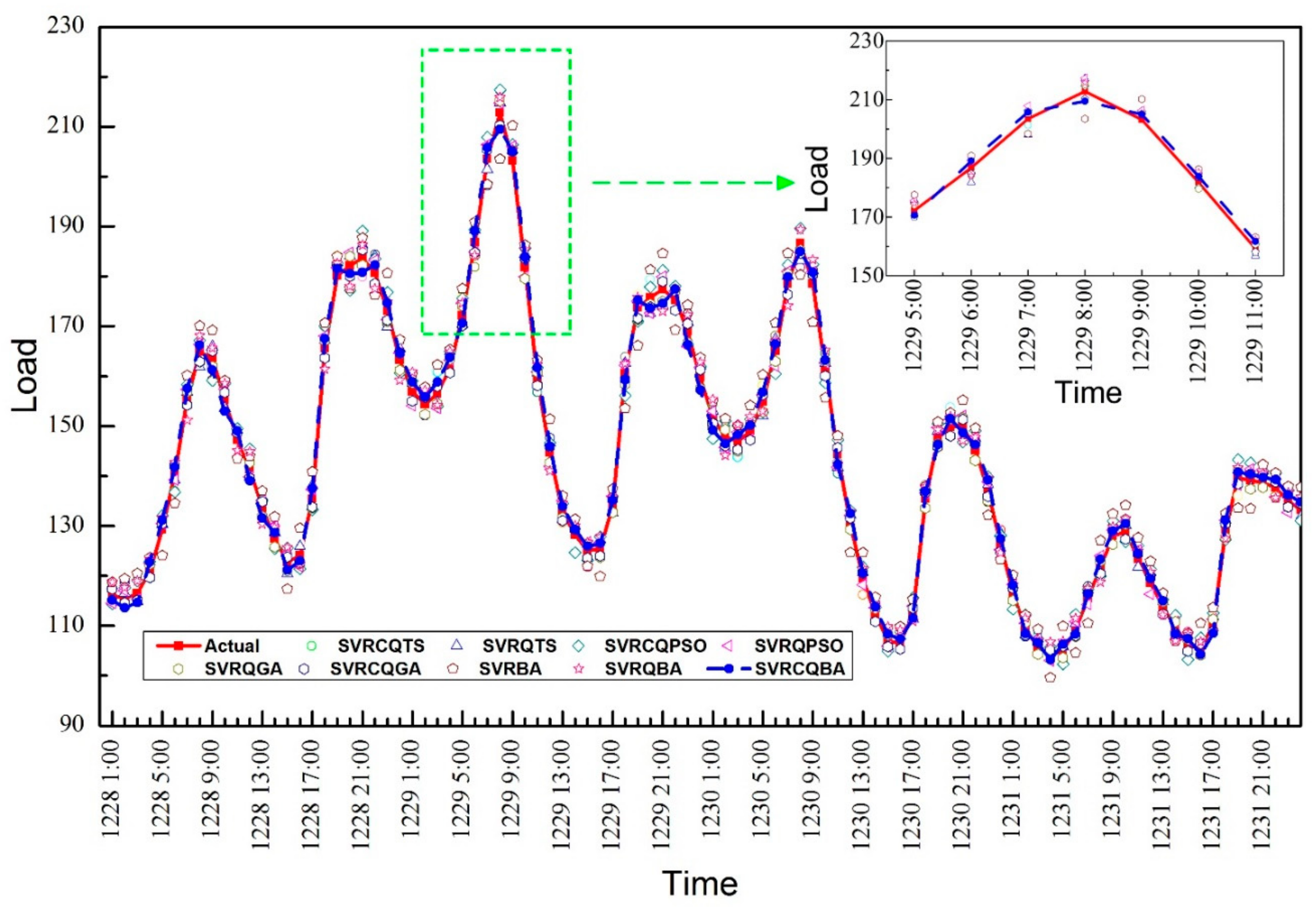
Based on the parameters combiation of each compared SVR-based model, use the training data set to conduct the training work, and receive the well trained SVR model. These trained models are further employed to forecast the load. The forecasting comparison curves of nine models mentioned above and actual values are shown as in Figure 2.

Table 2. Forecasting indexes of SVRCQBA and other alternative compared models.

Indexes	SVRQPSO [43]	SVRCQPSO [43]	SVRQTS [44]	SVRCQTS [44]	SVRQGA [45]	SVRCQGA [45]
MAPE (%)	1.9600	1.3200	1.8900	1.2900	1.7500	1.1700
RMSE	2.9358	1.9909	2.8507	1.9257	1.6584	1.4927
MAE	2.8090	1.8993	2.7181	1.8474	1.6174	1.4522
Indexes	SVRBA		SVRQBA		SVRCQBA
MAPE (%)	3.1600		1.7442		1.0982
RMSE	4.7312		2.5992		1.4835
MAE	4.5234		2.4968		1.4372

illustrates the forecasting accurate indexes for the proposed SVRCQBA and other alternative compared models.

Figure 2 clearly demonstrates that the proposed SVRCQBA model achieves results closer to the actual load values than other alternative compared models. In Table 2, the MAPE, RMSE and MAE of the proposed SVRCQBA model are 1.0982%, 1.4835, and 1.4372, respectively, which are smaller than that of other eight compared models. It also indicates that the proposed SVRCQBA model provides very contributions of improvements in terms of load forecasting accuracy. The concrete analysis results are as follows.

For forecasting performance comparison between SVRQBA and SVRBA models, the values of RMSE, MAPE and MAE for the SVRQBA model are smaller than that of the SVRBA model. It demonstrates that empowering the bats to have quantum behaviors, i.e., using quantum revolving gate (Equation (23)) in the BA to let any bats have comprehensive flying direction choices, which is an appropriate method to improve the solution, then, to improve the forecasting accuracy while the BA is hybridized with an SVR model. For example, in Table 2, the introduction of the quantum computing mechanism changes the forecasting performances (MAPE = 3.1600%, RMSE = 4.7312, MAE = 4.5234) of SVRBA model to much better performances (MAPE = 1.7442%, RMSE = 2.5992, MAE = 2.4968) of SVRQBA model. Employing the quantum revolving gate could improve almost 1.5% (=3.1600% − 1.7442%) forecasting accuracy in terms of MAPE, which plays the critical role in forecasting accuracy improvement contributions. Therefore, it is important to look for any more advanced quantum gates to empower more selection choices for any bats in the searching processes.

Meanwhile, comparing the RMSE, MAPE, MAE of SVRCQBA model with that of SVRQBA model, the forecasting accuracy of SVRCQBA model is superior to that of SVRQBA model. It reveals that the CQBA determines more appropriate parameters combination for an SVR model by introducing cat mapping function, which has a critical role in looking for an improved solution when the QBA algorithm are trapped in local optima or requires a long time to solve the problem of interest. For example, as shown in Table 2, searching parameters for an SVR model by CQBA instead of by QBA is excellently to shift the performances (MAPE = 1.7442%, RMSE = 2.5992, MAE = 2.4968) of the SVRQBA model to much better performances (MAPE = 1.0982%, RMSE = 1.4835, MAE = 1.4372) of the SVRCQBA model. Applying cat mapping function could improve almost 0.7% (=1.7442% − 1.0982%) forecasting accuracy in terms of MAPE, which also reveals the very contributions in forecasting accuracy improvement. Therefore, it is also an interesting issue to use other novel chaotic mapping functions to effectively enrich the diversity of population while searching iterations reach to a large scale.

In addition, the forecasting indexes results in Table 2 also illustrate that employing the CQPSO, CQTS, and CQGA, it could receive the best solution, ($\sigma$, C, $\epsilon$) = (19.000, 35.000, 0.820), ($\sigma$, C, $\epsilon$) = (12.000, 26.000, 0.320), and ($\sigma$, C, $\epsilon$) = (6.000, 54.000, 0.620), with forecasting error, (MAPE = 1.3200%, RMSE = 1.9909, MAE = 1.8993), (MAPE = 1.2900%, RMSE = 1.9257, MAE = 1.8474), and (MAPE = 1.1700%, RMSE = 1.4927, MAE = 1.4522), respectively. As mentioned above that it is superior to classical TS, PSO, and GA algorithms. However, the solution still could be further improved by the CQBA algorithm to ($\sigma$, C, $\epsilon$) = (11.000, 76.000, 0.670) with more accurate forecasting performance, (MAPE = 1.0982%, RMSE = 1.4835, MAE = 1.4372). It illustrates that hybridizing the cat mapping function and quantum computing mechanism with BA to select suitable parameters combination of an SVR model is a more powerful approach to receive satisfied the forecasting accuracy. Therefore, hybridizing CQBA with an SVR model could only improve at most 0.22% (=1.3200% − 1.0982%) forecasting accuracy in terms of MAPE, which also reveals the selection of advanced evolutionary algorithms could also contribute to forecasting accuracy improvements, however, along with the mature development of evolutionary algorithms, the contributions seem to be minor. Therefore, it should be a valuable remark that hybridizing other optimization approaches (such as chaotic mapping functions, quantum computing mechanism, cloud theory, and so on) to targeted overcome some embedded drawbacks of existed evolutionary algorithms is with much contributions to forecasting accuracy improvements. Based on the remark, it indicates that hybridizing novel optimization techniques with novel evolutionary algorithms could be the most important research tendency in the SVR-based load forecasting work.

Finally to ensure the significant contribution in terms of forecasting accuracy improvement for the proposed SVRQBA and SVRCQBA models the Wilcoxon signed-rank test is then implemented. In this paper the test is conducted under two significant levels α = 0.025 and α = 0.005 by one-tail test. The test results are demonstrated in

Table 3. Results of Wilcoxon signed-rank test.

Compared Models	Wilcoxon Signed-Rank Test
	α = 0.025; W = 2328	α = 0.005; W = 2328	p-Value
SVRCQBA vs. SVRQPSO	1087 T	1087 T	0.00220 **
SVRCQBA vs. SVRCQPSO	1184 T	1184 T	0.00156 **
SVRCQBA vs. SVRQTS	1123 T	1123 T	0.00143 **
SVRCQBA vs. SVRCQTS	1246 T	1246 T	0.00234 **
SVRCQBA vs. SVRQGA	1207 T	1207 T	0.00183 **
SVRCQBA vs. SVRCQGA	1358 T	1358 T	0.00578 *
SVRCQBA vs. SVRBA	874 T	874 T	0.00278 **
SVRCQBA vs. SVRQBA	1796 T	1796 T	0.00614 *

^T Denotes that the SVRCQGA model significantly outperforms the other alternative compared models; * represents that the test has rejected the null hypothesis under α = 0.025.; ** represents that the test has rejected the null hypothesis under α = 0.005.

which indicate that the proposed SVRCQBA model has received significant forecasting performance than other alternative compared models.

4. Conclusions

This paper proposes an electric demand forecasting by hybridizing SVR model with the cat mapping function quantum computing mechanism and the BA. The experimental results illustrate that the proposed model demonstrates significant forecasting performance than other hybrid chaotic quantum evolutionary algorithm SVR-based forecasting models in the literature. This paper continues to extend the search space with the limitations from conventional Newtonian dynamics by using quantum computing mechanism and to enhance ergodicity of population and to enrich the diversity of the searching space by using cat mapping function. Consequently, quantum computing mechanism is applied to endow bits to act as quantum behaviors hence to extend the searching space of BA and eventually to improve forecasting accuracy. Cat mapping function is further used to avoid premature convergence while the QBA is modeling and also contribute to accurate forecasting performances.

This paper also provides some important conclusions and indicates some valuable research directions for future research. Firstly, empowering the bats to have quantum behaviors by using quantum revolving gate could contribute most accuracy improvements. Therefore, in the future the successive researchers could consider constructing an n-dimensional quantum gate where n is the dimensions of employed data set i.e., for each bat in the modeling process it has n probability amplitudes instead of only one amplitude. Based on this new design it is expected to look for more abundant search results via those bats with n probability amplitudes.

Secondly applying chaotic mapping functions could also improve forecasting accuracy. Therefore, in the future any approaches which could enrich the diversity of population during modeling process are deserved to employ to receive more satisfied forecasting accuracy such as other novel chaotic mapping functions or novel design of mutation or crossover operations and so on.

Finally, only hybridizing different evolutionary algorithms could contribute minor forecasting accuracy improvements. Therefore, hybridizing different novel optimization techniques with novel evolutionary algorithms could contribute most in terms of forecasting accuracy improvements and would be the most important research tendency in the SVR-based load forecasting work in the future.

References

- Xiao, L.; Wang, J.; Hou, R.; Wu, J. A combined model based on data pre-analysis and weight coefficients optimization for electrical load forecasting. Energy 2015, 82, 524–549. [Google Scholar] [CrossRef]
- Bunn, D.W.; Farmer, E.D. Comparative models for electrical load forecasting. Int. J. Forecast. 1986, 2, 241–242. [Google Scholar]
- Fan, G.; Peng, L.-L.; Hong, W.-C.; Sun, F. Electric load forecasting by the SVR model with differential empirical mode decomposition and auto regression. Neurocomputing 2016, 173, 958–970. [Google Scholar] [CrossRef]
- Wang, J.; Wang, J.; Li, Y.; Zhu, S.; Zhao, J. Techniques of applying wavelet de-noising into a combined model for short-term load forecasting. Int. J. Electr. Power Energy Syst. 2014, 62, 816–824. [Google Scholar] [CrossRef]
- Pappas, S.S.; Ekonomou, L.; Karampelas, P.; Karamousantas, D.C.; Katsikas, S.K.; Chatzarakis, G.E.; Skafidas, P.D. Electricity demand load forecasting of the Hellenic power system using an ARMA model. Electr. Power Syst. Res. 2010, 80, 256–264. [Google Scholar] [CrossRef]
- Zhang, M.; Bao, H.; Yan, L.; Cao, J.; Du, J. Research on processing of short-term historical data of daily load based on Kalman filter. Power Syst. Technol. 2003, 9, 39–42. [Google Scholar]
- Maçaira, P.M.; Souza, R.C.; Oliveira, F.L.C. Modelling and forecasting the residential electricity consumption in Brazil with pegels exponential smoothing techniques. Procedia Comput. Sci. 2015, 55, 328–335. [Google Scholar] [CrossRef]
- Dudek, G. Pattern-based local linear regression models for short-term load forecasting. Electr. Power Syst. Res. 2016, 130, 139–147. [Google Scholar] [CrossRef]
- Zhang, W.; Yang, J. Forecasting natural gas consumption in China by Bayesian model averaging. Energy Rep. 2015, 1, 216–220. [Google Scholar] [CrossRef]
- Li, H.Z.; Guo, S.; Li, C.J.; Sun, J.Q. A hybrid annual power load forecasting model based on generalized regression neural network with fruit fly optimization algorithm. Knowl.-Based Syst. 2013, 37, 378–387. [Google Scholar] [CrossRef]
- Ertugrul, Ö.F. Forecasting electricity load by a novel recurrent extreme learning machines approach. Int. J. Electr. Power Energy Syst. 2016, 78, 429–435. [Google Scholar] [CrossRef]
- Bennett, C.J.; Stewart, R.A.; Lu, J.W. Forecasting low voltage distribution network demand profiles using a pattern recognition based expert system. Energy 2014, 67, 200–212. [Google Scholar] [CrossRef]
- Akdemir, B.; Çetinkaya, N. Long-term load forecasting based on adaptive neural fuzzy inference system using real energy data. Energy Procedia 2012, 14, 794–799. [Google Scholar] [CrossRef]
- Hooshmand, R.-A.; Amooshahi, H.; Parastegari, M. A hybrid intelligent algorithm based short-term load forecasting approach. Int. J. Electr. Power Energy Syst. 2013, 45, 313–324. [Google Scholar] [CrossRef]
- Mahmoud, T.S.; Habibi, D.; Hassan, M.Y.; Bass, O. Modelling self-optimised short term load forecasting for medium voltage loads using tunning fuzzy systems and artificial neural networks. Energy Convers. Manag. 2015, 106, 1396–1408. [Google Scholar] [CrossRef]
- Niu, D.X.; Shi, H.; Wu, D.D. Short-term load forecasting using Bayesian neural networks learned by hybrid Monte Carlo algorithm. Appl. Soft Comput. 2012, 12, 1822–1827. [Google Scholar] [CrossRef]
- Hanmandlu, M.; Chauhan, B.K. Load forecasting using hybrid models. IEEE Trans. Power Syst. 2011, 26, 20–29. [Google Scholar] [CrossRef]
- Li, S.; Wang, P.; Goel, L. Short-term load forecasting by wavelet transform and evolutionary extreme learning machine. Electr. Power Syst. Res. 2015, 122, 96–103. [Google Scholar] [CrossRef]
- Lou, C.W.; Dong, M.C. A novel random fuzzy neural networks for tackling uncertainties of electric load forecasting. Int. J. Electr. Power Energy Syst. 2015, 73, 34–44. [Google Scholar] [CrossRef]
- Suykens, J.A.K.; Vandewalle, J.; De Moor, B. Optimal control by least squares support vector machines. Neural Netw. 2001, 14, 23–35. [Google Scholar] [CrossRef]
- Sankar, R.; Sapankevych, N.I. Time series prediction using support vector machines: A survey. IEEE Comput. Intell. Mag. 2009, 4, 24–38. [Google Scholar]
- Vapnik, V. The Nature of Statistical Learning Theory, 2nd ed.; Springer: New York, NY, USA, 2000; ISBN 978-0-387-98780-4. [Google Scholar]
- Vapnik, V. Statistical Learning Theory; Wiley: New York, NY, USA, 1998; ISBN 978-0-471-03003-4. [Google Scholar]
- Scholkopf, B.; Smola, A.J. Learning with Kernels: Support Vector Machines, Regularization, Optimization, and Beyond; The MIT Press: Cambridge, MA, USA, 2002; ISBN 978-0-262-19475-4. [Google Scholar]
- Vapnik, V.; Golowich, S.; Smola, A. Support vector machine for function approximation, regression estimation, and signal processing. Adv. Neural Inf. Process. Syst. 1996, 9, 281–287. [Google Scholar]
- Antonanzas, J.; Urraca, R.; Martinez-De-Pison, F.J.; Antonanzas-Torres, F. Solar irradiation mapping with exogenous data from support vector regression machines estimations. Energy Convers. Manag. 2015, 100, 380–390. [Google Scholar] [CrossRef]
- Yu, P.S.; Chen, S.T.; Chang, I.F. Support vector regression for real-time flood stage forecasting. J. Hydrol. 2006, 328, 704–716. [Google Scholar] [CrossRef]
- Pai, P.-F.; Hong, W.-C. A recurrent support vector regression model in rainfall forecasting. Hydrol. Process. 2007, 21, 819–827. [Google Scholar] [CrossRef]
- Granata, F.; Gargano, R.; de Marinis, G. Support vector regression for rainfall-runoff modeling in urban drainage: A comparison with the EPA’s storm water management model. Water 2016, 8, 69. [Google Scholar] [CrossRef]
- Granata, F.; Papirio, S.; Esposito, G.; Gargano, R.; de Marinis, G. Machine learning algorithms for the forecasting of wastewater quality indicators. Water 2017, 9, 105. [Google Scholar] [CrossRef]
- Kavaklioglu, K. Modeling and prediction of Turkey’s electricity consumption using Support Vector Regression. Appl. Energy 2011, 88, 368–375. [Google Scholar] [CrossRef]
- Hong, W.C. Electric load forecasting by seasonal recurrent SVR (support vector regression) with chaotic artificial bee colony algorithm. Energy 2011, 36, 5568–5578. [Google Scholar] [CrossRef]
- Hong, W.-C.; Dong, Y.; Zhang, W.; Chen, L.-Y.; Panigrahi, B.K. Cyclic electric load forecasting by seasonal SVR with chaotic genetic algorithm. Int. J. Electr. Power Energy Syst. 2013, 44, 604–614. [Google Scholar] [CrossRef]
- Ju, F.-Y.; Hong, W.-C. Application of seasonal SVR with chaotic gravitational search algorithm in electricity forecasting. Appl. Math. Model. 2013, 37, 9643–9651. [Google Scholar] [CrossRef]
- Geng, J.; Huang, M.-L.; Li, M.-W.; Hong, W.-C. Hybridization of seasonal chaotic cloud simulated annealing algorithm in a SVR-based load forecasting model. Neurocomputing 2015, 151, 1362–1373. [Google Scholar] [CrossRef]
- Peng, L.-L.; Fan, G.-F.; Huang, M.-L.; Hong, W.-C. Hybridizing DEMD and quantum PSO with SVR in electric load forecasting. Energies 2016, 9, 221. [Google Scholar] [CrossRef]
- Yang, X.-S. A new metaheuristic bat-inspired algorithm. In Nature Inspired Cooperative Strategies for Optimization; González, J.R., Pelta, D.A., Cruz, C., Terrazas, G., Krasnogor, N., Eds.; Springer: Berlin/Heidelberg, Germany, 2010; Volume 284, pp. 65–74. ISBN 978-3-642-12537-9. [Google Scholar]
- Yang, X.-S. Nature Inspired Meta-heuristic Algorithms, 2nd ed.; Luniver Press: Frome, UK, 2010; pp. 97–104. ISBN 978-1-905986-28-6. [Google Scholar]
- Sheng, X.-H.; Ye, C.-M. Application of bat algorithm to permutation flow-shop scheduling problem. Ind. Eng. J. 2013, 16, 119–124. [Google Scholar]
- Komarasamy, G.; Wahi, A. An optimized k-means clustering technique using bat algorithm. Eur. J. Sci. Res. 2012, 84, 263–273. [Google Scholar]
- Yang, X.-S.; Gandomi, A.H. Bat algorithm: A novel approach for global engineering optimization. Eng. Comput. 2012, 29, 464–483. [Google Scholar] [CrossRef]
- Yang, X.-S. Bat algorithm for multi-objective optimization. Int. J. Bio-Inspired Comput. 2011, 3, 267–274. [Google Scholar] [CrossRef]
- Huang, M.-L. Hybridization of chaotic quantum particle swarm optimization with SVR in electric demand forecasting. Energies 2016, 9, 426. [Google Scholar] [CrossRef]
- Lee, C.-W.; Lin, B.-Y. Application of hybrid quantum tabu search with support vector regression (SVR) for load forecasting. Energies 2016, 9, 873. [Google Scholar] [CrossRef]
- Lee, C.-W.; Lin, B.-Y. Applications of the chaotic quantum genetic algorithm with support vector regression in load forecasting. Energies 2017, 10, 1832. [Google Scholar] [CrossRef]
- Li, Z.-Y.; Ma, L.; Zhang, H.-Z. Quantum bat algorithm for function optimization. J. Syst. Manag. 2014, 23, 717–722. [Google Scholar]
- Moss, C.F.; Sinha, S.R. Neurobiology of echolocation in bats. Curr. Opin. Neurobiol. 2003, 13, 751–758. [Google Scholar] [CrossRef] [PubMed]
- Yuan, X.; Wang, P.; Yuan, Y.; Huang, Y.; Zhang, X. A new quantum inspired chaotic artificial bee colony algorithm for optimal power flow problem. Energy Convers. Manag. 2015, 100, 1–9. [Google Scholar] [CrossRef]
- Peng, A.N. Particle swarm optimization algorithm based on chaotic theory and adaptive inertia weight. J. Nanoelectron. Optoelectron. 2017, 12, 404–408. [Google Scholar] [CrossRef]
- Li, M.-W.; Geng, J.; Hong, W.-C.; Chen, Z.-Y. A novel approach based on the Gauss-vSVR with a new hybrid evolutionary algorithm and input vector decision method for port throughput forecasting. Neural Comput. Appl. 2017, 28, S621–S640. [Google Scholar] [CrossRef]
- Li, M.-W.; Hong, W.-C.; Geng, J.; Wang, J. Berth and quay crane coordinated scheduling using chaos cloud particle swarm optimization algorithm. Neural Comput. Appl. 2017, 28, 3163–3182. [Google Scholar] [CrossRef]
- Global Energy Forecasting Competition. 2014. Available online: http://www.drhongtao.com/gefcom/ (accessed on 28 November 2017).
- Diebold, F.X.; Mariano, R.S. Comparing predictive accuracy. J. Bus. Econ. Stat. 1995, 13, 134–144. [Google Scholar]
- Derrac, J.; García, S.; Molina, D.; Herrera, F. A practical tutorial on the use of nonparametric statistical tests as a methodology for comparing evolutionary and swarm intelligence algorithms. Swarm Evol. Comput. 2011, 1, 3–18. [Google Scholar] [CrossRef]
- Wilcoxon, F. Individual comparisons by ranking methods. Biom. Bull. 1945, 1, 80–83. [Google Scholar] [CrossRef]
Figure 1.
Chaotic quantum bat algorithm flowchart.
Figure 2.
Forecasting values of SVRCQBA and other alternative compared models.