Parallel Multi-Objective Genetic Algorithm for Short-Term Economic Environmental Hydrothermal Scheduling

Abstract

With the increasingly serious energy crisis and environmental pollution, the short-term economic environmental hydrothermal scheduling (SEEHTS) problem is becoming more and more important in modern electrical power systems. In order to handle the SEEHTS problem efficiently, the parallel multi-objective genetic algorithm (PMOGA) is proposed in the paper. Based on the Fork/Join parallel framework, PMOGA divides the whole population of individuals into several subpopulations which will evolve in different cores simultaneously. In this way, PMOGA can avoid the wastage of computational resources and increase the population diversity. Moreover, the constraint handling technique is used to handle the complex constraints in SEEHTS, and a selection strategy based on constraint violation is also employed to ensure the convergence speed and solution feasibility. The results from a hydrothermal system in different cases indicate that PMOGA can make the utmost of system resources to significantly improve the computing efficiency and solution quality. Moreover, PMOGA has competitive performance in SEEHTS when compared with several other methods reported in the previous literature, providing a new approach for the operation of hydrothermal systems.

1. Introduction

Along with the rapid development of global economy over the past several decades, the power demand has increased continuously, and a large amount of hydro and thermal plants have been successively built to supply sufficient energy [1,2,3]. However, thermal plants inevitably produce emissions of pollutants like sulfur oxide and nitrogen oxide, which gives rise to a series of serious environmental problems and high social economic costs [4,5,6]. Given to strong awareness about sustainable development, short-term economic environmental hydrothermal scheduling (SEEHTS) is becoming one of the most important optimization problems in modern electrical power systems [7]. The main aim of SEEHTS is to choose the optimal operational process in a scheduling period to minimize the total fuel cost and pollutant emission cost simultaneously, while satisfying a group of equality and inequality constraints imposed on the system, including generation limits of hydro and thermal plants, storage and discharge limits and hydraulic balance of hydro plants, and load balance. Hence, due to the coupling characteristics in constraints and the competitiveness between objectives, SEEHTS becomes a high-dimensional multi-objective constrained optimization problem [7,8].

Many researchers have been applying every effort to develop efficient optimization algorithms to solve the SEEHTS problem. These methods can be roughly divided into two categories: one is single-objective optimization algorithms and the other is multi-objective optimization algorithms [9]. The former methods usually use the method of weighting, target or constraints conversion to transform the SEEHTS into a single-objective problem, then use standard mathematical methods, like linear programming or nonlinear programming to solve it. Although a great deal of computation can be avoided in most cases, there are such issues as sensitivity to transformation coefficients, high memory requirements, and difficulty to obtain compromise solution sets in one trial [10].

On the other hand, the latter mainly use multi-objective evolutionary algorithms (MOEAs) such as the multi-objective genetic algorithm (MOGA), multi-objective particle swarm optimization, multi-objective gravitational search algorithm, and multi-objective differential evolution to handle the SEEHTS problem [11,12]. The MOEAs have no strict requirements on the continuity and differentiability of optimization problems, and usually are able to obtain Pareto solution sets rather than one solution in a single run [13]. However, due to the stochastic optimization mechanism, MOEAs may suffer from the problems of premature convergence and solution volatility [14,15,16]. Sometimes, the satisfactory Pareto solutions cannot be obtained. In addition, when the problem scale reaches a certain large degree, the population diversity and computation cost will be intolerable [17,18,19]. Thus, there is some space to improve MOEAs for the SEEHTS problem. In general, we can modify the search mechanism of MOEAs or use advanced computer technologies to alleviate these defects [20,21]. Here, parallel technologies are used to enhance the performance of MOEAs.

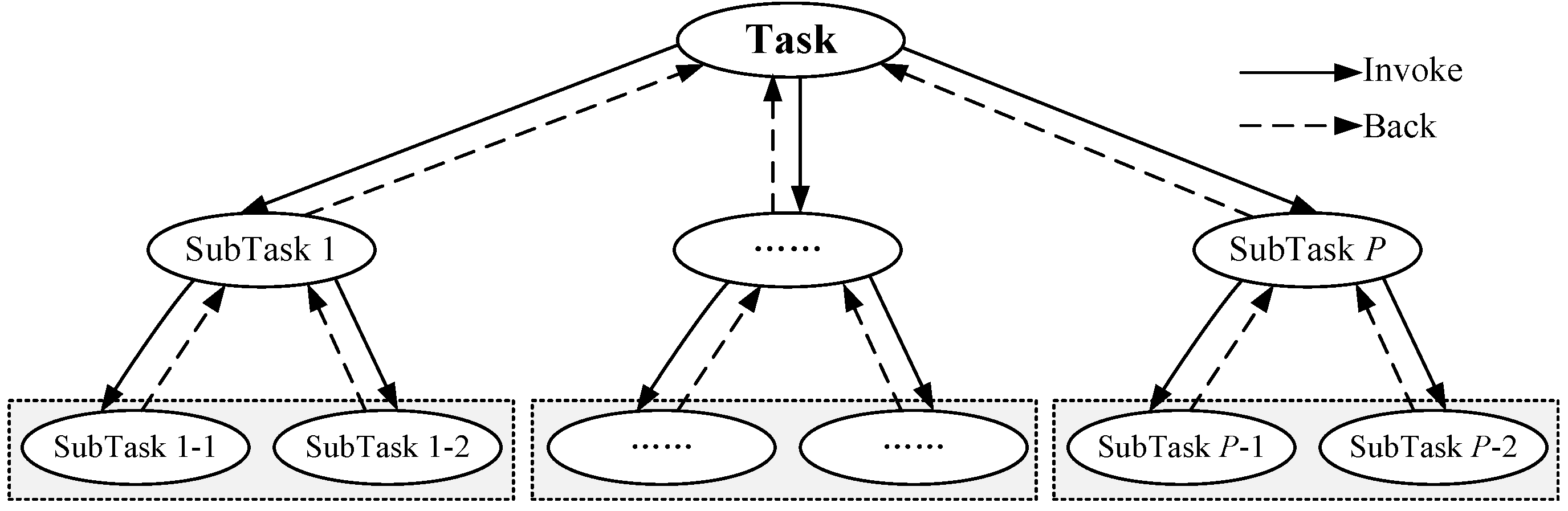
Recently, with the increasing popularity of multi-core technology, multi-core processors have become the standard configuration of personal computers, workstations and servers, providing the essential hardware conditions for the implementation of parallelization [22,23]. For parallel computation in multi-core computers, the large computational task is divided into several smaller subtasks to be concurrently executed in different cores [20], which can help shorten the computing time and improve the resource utilization efficiency [24]. Nowadays, multi-core parallel computing technology is a hot research area achieving great success in the fields of scientific research and engineering practice [21,25]. However, to our knowledge, there are a few reports about using the multi-core parallel technology to solve the SEEHTS problem. Therefore, it is of great importance to develop parallel optimization algorithms for the SEEHTS problem, and in the paper, we focus on the multi-core parallelization of MOEAs to solve the complicated SEEHTS problem.

To achieve parallel computing, many parallel frameworks have been developed by different companies or institutions, such as Fork/Join, open multi-processing and message passing interface [21]. Since the parallel framework can have a significant impact on the performance of parallel algorithms, we should take many factors into consideration when choosing the framework, such as programming language and operating environment [26,27]. Here, given that our algorithms are encoded in Java language, for the ease of implementation, the Fork/Join framework is used for the realization of algorithm parallelization [24,28]. As a standard Java parallel program platform, Fork/Join can help programmers design parallel optimization algorithms with cross-platform advantages. 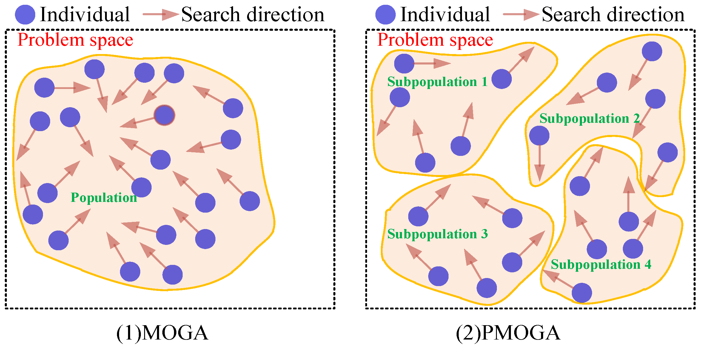Based on the non-dominated sorting genetic algorithm-II (NSGA-II) [17,29,30,31], the parallel multi-objective genetic algorithm (PMOGA) which combines the merits of NSGA-II and parallel computing is proposed. Finally, PMOGA is applied to a mature hydrothermal system consisting of four hydro plants and three thermal plants. The results from different cases show that the proposed approach has better convergence speed and Pareto optimal front performance than traditional methods, demonstrating the effectiveness of our methods.

Moreover, to clearly understand our work, the contributions of this paper can be summarized as: (1) an optimization model is presented for SEEHTS; (2) a novel PMOGA combining the advantages of MOGA and parallel techniques is proposed to enhance the computational efficiency and population diversity simultaneously; (3) a new heuristic constraint handling method based on the two-stage proportional adjustment idea is proposed to ensure the feasibility of solutions; and (4) our method outperforms several other methods, which proves to be an alternative tool for the SEEHTS problem.

The rest of this paper is organized as follows. Section 2 introduces the mathematical model for the SEEHTS problem. Section 3 presents the proposed PMOGA method. Section 4 gives the details of PMOGA for the SEEHTS problem. Section 5 provides the experimental results and discussions. Section 6 presents the conclusions.

2. Problem Formulation

2.1. Object Function

Since the short-term hydrothermal system scheduling minimizes both environmental pollutant and economic costs simultaneously, the optimization objectives can be described as follows:

$$\min \hspace{0.17em}\left(f_{eco},f_{emi}\right)$$

(1)

where f_eco ($) and f_emi (lb) denote the total economic cost and environmental cost, respectively.

2.1.1. Economic Objective

Generally, the fuel cost for thermal plants can be seen as the sum of a quadratic and a sinusoidal function representing the valve-point effect. The economic objective is to minimize the total fuel cost of hydrothermal system over the planning period, which can be described as follows:

$$\min \hspace{0.17em}{f}_{eco}={\displaystyle \sum _{i=1}^{N_T}{\displaystyle \sum _{j=1}^J{f}_i\left(P_{Ti}^j\right)}}={\displaystyle \sum _{i=1}^{N_T}{\displaystyle \sum _{j=1}^J\left\{a_i+b_i\cdot P_{Ti}^j+c_i\cdot {\left(P_{Ti}^j\right)}^2+\left|d_i\cdot \sin \left[e_i\cdot \left(P_{Ti}^{\min }-P_{Ti}^j\right)\right]\right|\right\}}}$$

(2)

where N_T is the number of thermal plants; J is the number of time intervals; $P_{Ti}^j$ is the power generation of the i-th thermal plant at the j-th interval in MW; $f_i\left(P_{Ti}^j\right)$ denotes the fuel cost function of the i-th thermal plant at the j-th interval in $; a_i ($/h), b_i ($/MWh), c_i ($/(MW)²h), d_i ($/h) and e_i (1/MW) are the fuel coefficients of the i-th thermal plant , respectively; $P_{Ti}^{\min }$ is the minimum power of the i-th thermal plant in MW.

2.1.2. Environmental Objective

Compared to hydropower plants, thermal plants may produce some atmospheric pollution during power generation. Thus, the environmental objective is to minimize the total emission pollutants of thermal generators as much as possible, which can be expressed as follows:

$$\min \hspace{0.17em}{f}_{emi}={\displaystyle \sum _{i=1}^{N_T}{\displaystyle \sum _{j=1}^J{e}_i\left(P_{Ti}^j\right)}}={\displaystyle \sum _{i=1}^{N_T}{\displaystyle \sum _{j=1}^J\left\{{\mathsf{\alpha }}_i+{\mathsf{\beta }}_i\cdot P_{Ti}^j+{\mathsf{\gamma }}_i\cdot {\left(P_{Ti}^j\right)}^2+{\mathsf{\eta }}_i\cdot \exp \left({\mathsf{\theta }}_i\cdot P_{Ti}^j\right)\right\}}}$$

(3)

where $e_i\left(P_{Ti}^j\right)$ is the emission cost function of the i-th thermal plant at the j-th interval in lb. α_i (lb/h), β_i (lb/MWh), γ_i (lb/(MW)²h), η_i (lb/h) and θ_i (1/MW) are the emission coefficients of the i-th thermal plant , respectively.

2.2. Constraints

In SEEHTS, a large amount of equality and inequality constraints must be considered, such as water and load balances, reservoir discharge rates, and technical constraints for hydro or thermal generators. Besides, for the purposed of persistence, the variable units are the same as those in [32,33].

2.2.1. Power Balance Constraints

$${\displaystyle \sum _{i=1}^{N_T}{P}_{Ti}^j}+{\displaystyle \sum _{k=1}^{N_H}{P}_{Hk}^j}=P_D^j+P_L^j,\hspace{0.17em}\hspace{0.17em}\hspace{0.17em}j\in \left[1,J\right]$$

(4)

where N_H is number of hydro plants in system; $P_D^j$ is the system load at the jth interval in MW; $P_L^j$ is the power transmission loss at the j-th interval in MW, which is described as follows:

$$P_L^j={\displaystyle \sum _{i=1}^{N_T+N_H}{\displaystyle \sum _{m=1}^{N_T+N_H}{P}_i^j\cdot B_{2i}^m\cdot P_m^j}+}{\displaystyle \sum _{i=1}^{N_T+N_H}{B}_{1i}\cdot P_i^j+B_0},\hspace{0.17em}\hspace{0.17em}\hspace{0.17em}j\in \left[1,J\right]$$

(5)

where $P_m^j$ denotes the power generation of the m-th plants in system at the j-th interval in MW; $B_{2i}^m, B_{1i}^m$ and B₀ (MW) represent the power transmission loss coefficients, respectively.

Furthermore, $P_{Hk}^j$ denotes the power output of the kth hydro plant at the j-th interval in MW, which is a quadratic function of water discharge and storage volumes as follows [32,34]:

$$P_{Hk}^j=C_{k1}\cdot {\left(V_{Hk}^j\right)}^2+C_{k2}\cdot {\left(Q_{Hk}^j\right)}^2+C_{k3}\cdot V_{Hk}^j\cdot Q_{Hk}^j+C_{k4}\cdot V_{Hk}^j+C_{k5}\cdot Q_{Hk}^j+C_{k6},\hspace{0.17em}\hspace{0.17em}\hspace{0.17em}j\in \left[1,J\right]$$

(6)

where C_k1, C_k2, C_k3, C_k4, C_k5 and C_k6 represent the generation coefficients of the k-th hydro plant, respectively. The units of C_k1, C_k2 and C_k3 are respectively MW/(10⁴·m³)², the units of C_k4 and C_k5 are respectively MW/10⁴·m³, while the unit of C_k6 is MW. $V_{Hk}^j$ is the initial storage of the k-th hydro plant at the j-th interval in 10⁴·m³. $Q_{Hk}^j$ is the water discharge of the k-th hydro plant at the j-th interval in 10⁴·m³.

2.2.2. Thermal Plant Power Output Capacity Constraints

$$P_{Ti}^{j,\min }\le P_{Ti}^j\le P_{Ti}^{j,\max },\hspace{0.17em}\hspace{0.17em}i\in \left[1,N_T\right],\hspace{0.17em}\hspace{0.17em}\hspace{0.17em}j\in \left[1,J\right]$$

(7)

where $P_{Ti}^{j,\max }$ and $P_{Ti}^{j,\min }$ are the maximum and minimum power output of the i-th thermal plant at the j-th interval in MW, respectively.

2.2.3. Hydro Plant Power Output Capacity Constraints

$$P_{Hk}^{j,\min }\le P_{Hk}^j\le P_{Hk}^{j,\max },\hspace{0.17em}k\in \left[1,N_H\right],\hspace{0.17em}\hspace{0.17em}j\in \left[1,J\right]$$

(8)

where $P_{Hk}^{j,\max }$ and $P_{Hk}^{j,\min }$ are the maximum and minimum power output of the k-th hydro plant at the j-th interval in MW, respectively.

2.2.4. Reservoir Storage Volume Constraints

$$V_{Hk}^{j,\min }\le V_{Hk}^j\le V_{Hk}^{j,\max },\hspace{0.17em}\hspace{0.17em}\hspace{0.17em}\hspace{0.17em}k\in \left[1,N_H\right],j\in \left[1,J\right]$$

(9)

where $V_{Hk}^{j,\max }$and $V_{Hk}^{j,\min }$ represent the maximum and minimum storage volume of the k-th hydro plant at the j-th interval in 10⁴·m³, respectively.

2.2.5. Water Discharge Constraints

$$Q_{Hk}^{j,\min }\le Q_{Hk}^j\le Q_{Hk}^{j,\max },\hspace{0.17em}\hspace{0.17em}\hspace{0.17em}\hspace{0.17em}k\in \left[1,N_H\right],j\in \left[1,J\right]$$

(10)

where $Q_{Hk}^{j,\max }$ and $Q_{Hk}^{j,\min }$ represent the maximum and minimum water discharge of the k-th hydro plant at the j-th interval in 10⁴·m³, respectively.

2.2.6. Water Dynamic Balance Constraints

$$V_{Hk}^j=V_{Hk}^{j-1}+I_{Hk}^j+{\displaystyle \sum _{l\in {\Omega }_k}\left(Q_{Hl}^{j-{\tau }_l^k}+S_{Hl}^{j-{\tau }_l^k}\right)}-Q_{Hk}^j-S_{Hk}^j\hspace{0.17em},\hspace{0.17em}\hspace{0.17em}k\in \left[1,N_H\right],j\in \left[1,J\right]$$

(11)

where $I_{Hk}^j$ and $S_{Hk}^j$ represent the local inflow and water spillage of the k-th hydro plant at the j-th interval in 10⁴·m³, respectively. To be mentioned, for simplicity, it is assumed that all the water discharge is used for generation. ${\Omega }_k$ is the set of directly upstream hydro plants above the kth hydro plant. ${\mathsf{\tau }}_l^k$ is the water transport period from hydro plant l to k.

2.2.7. Initial and Terminal Storage Volume Constraints

$$\{\begin{array}{l}{V_{Hk}^j|}^{j=0}=V_{Hk}^{beg}\hspace{0.17em}\hspace{0.17em},k\in \left[1,N_H\right]\\ {V_{Hk}^j|}^{j=T}=V_{Hk}^{end}\hspace{0.17em}\hspace{0.17em},k\in \left[1,N_H\right]\end{array}$$

(12)

where $V_{Hk}^{\mathrm{beg}}$ and $V_{Hk}^{\mathrm{end}}$ are the initial storage volume and final storage volume of the k-th hydro plant in 10⁴·m³, respectively.

3. Parallel Multi-Objective Genetic Algorithm

3.1. Overview of Multi-Objective Genetic Algorithm

In fact, multi-objective optimization (MOO) has found many applications in the energy field. Without loss of generality, supposing that there are n objectives to be minimized, which is defined as f(x) = [f₁(x), f₂(x), …, f_n(x)], where f_i(x) is the ith objective and x is the decision vector. Generally, in MOO problems, no one solution is better than any other solutions with respect to all objectives. Hence, MOO aims at finding the Pareto optimal solution set consisting of alternative compromise solutions for all the objectives [31,35,36,37].

The non-dominated sorting genetic algorithm-II, NSGA-II for short, is one of the most classical multi-objective genetic algorithms used to solve MOO problems [30]. Due to its practicality and feasibility, NSGA-II is chosen as the method to be parallelized in this research. In the NSGA-II, each potential solution for the optimization problem at hand is treated as one individual surviving in nature. After randomly generating the initial population in the search space, three basic evolutionary operators—the selection operator, crossover operator and mutation operator—are used to produce the new population composed of elite individuals. Moreover, using the fast sorting method and crowding distance strategy, all the Pareto solutions obtained at each cycle will be dynamically updated [38,39]. The iterative process will be not stopped until the terminal condition is met, then the final individuals represent the approximate optimal Pareto solutions. The procedures of NSGA-II are briefly described as follows:

Step 1:

Preparation and initialization. Determine the necessary computational parameters of the algorithm, and generate the parent population randomly in the feasible space.

Step 2:

Calculate the objective function values and constraint violation value of each solution in the parent population.

Step 3:

Fast non-dominated sorting the parent population. Each solution is assigned a front level equal to its own non-domination level. Then, calculate the crowding distance value of all the individuals at each non-domination level, which will be used to sort the parent population in a descending order.

Step 4:

Selection operation. Two individuals randomly chosen from the hybrid population are compared, and the one with better front level and crowding distance value will be selected as the candidate solution in the mating pool.

Step 5:

Crossover and mutation operation. To enhance the population diversity, the predefined crossover operator and mutation operator will be used to generate the offspring population.

Step 6:

The parent population and offspring population are combined and sorted based on the non-domination and crowding distance. Then, the better solutions will be chosen as the members in the new generation.

Step 7:

Repeat Steps 2 to 6 until the maximum iteration is reached, then export the Pareto optimal solutions.

3.2. Fork/Join Parallel Framework

As a famous parallel framework based on the divide-and-conquer strategy, Fork/Join first divides the complicated computational task into a series of smaller subtasks to be simultaneously solved by simple methods, and then merges the solutions of all the subtasks to obtain the final optimal result of the original problem [20,26]. Figure 1 shows a diagram of the Fork/Join framework. In the Fork/Join framework, the threshold is used to control the scale of the subtasks and decide whether to implement the decomposition process. Thus, the threshold selection has direct impact on the performance of parallel methods: smaller value usually brings about heavy management expenses spent on subtasks, while larger value cannot make full use of the abundant multi-core resource in computers. Thus, the threshold value should be chosen carefully before the calculation. To obtain better parallelization performance, the threshold here is defined as follows:

$$T=\lceil a/P\rceil$$

(13)

where T is the threshold value; a is the scale of the parent task; P is the number of units for parallel computing; and $\lceil x\rceil$ represents the minimum integer bigger than x.

In Fork/Join, to reduce the extra cost caused by the frequent creation and closure of worker threads, the thread pool where the number of threads is equal to the number of cores is created at the beginning. During the parallel computation process, to avoid wasting multi-core resources, Fork/Join uses the work stealing technique to handle the work queue contention problem. Besides, as Fork/Join is an open source project, with little knowledge of the technical parallelization, programmers can call the universal application programming interface to develop procedures running in many operating systems that support Java virtual machine operation [26]. Thus, due to the above outstanding merits, Fork/Join is employed in this paper to realize the implementation of parallel algorithms for solving the SEEHTS problem.

3.3. Parallel Multi-Objective Genetic Algorithm

Although the NSGA-II algorithm has been successfully employed to solve multi-objective problems, this method still has some disadvantages: (1) considering the worst case of all operations, the overall complexity of NSGA-II exhibits an approximate square growth [30], i.e., O(M·N²), where M and N denote the number of objectives and individuals, respectively; (2) at the latter evolution process, the diversity of individuals will significantly reduce, and the population tends to emerge the premature convergence [29]. When handling large-scale engineering problems, NSGA-II may take a long computation time to finish the entire evolution process, but the pseudo Pareto optimal solutions are obtained in the end. Then, inspired by some earlier studies on the small population technique [40,41] and multi-core parallel technology [20,21], the PMOGA is proposed in this section to alleviate the above problems in MOGA.

Figure 2 shows a map of the population decomposition process in PMOGA, while the map of the PMOGA algorithm is given in Figure 3. In the PMOGA, the calculation of the original larger population is treated as the parent task. After the initialization step, the divide-and-conquer strategy is used to divide the task into several smaller subpopulations which will be executed simultaneously in different cores or threads. Each computing unit only answers for the task assigned by thread manager, and all the subpopulations start searching for the feasible Pareto solutions. The parallel processing will not be stopped until all subtasks finish the corresponding calculation task. Once the calculation of all subtasks is done, the main thread will collect the final Pareto solutions of all the subpopulations and choose the best individuals to form up the optimal Pareto solution set.

In summary, our method can combine the advantages of MOGA and parallel technique so as to enhance the population diversity and computational efficiency simultaneously. On the one hand, as shown in Figure 4, PMOGA can maintain the population diversity by dividing the whole population into several small subpopulations to search for Pareto solutions independently in the problem space. The small-population based strategy can help increase the exploitation and exploration ability of swarms and avoid the prematurity problem of MOGA as far as possible.

On the other hand, by using the parallel technique, PMOGA can reduce the execution time of population evolution significantly. Assume there are N individuals and M objectives, when PMOGA is performed in P units, the number of individuals in each subpopulation is about N/P, and the complexity of each subtask is reduced to O(M·(N/P)²), which indicates that PMOGA lowers the computational complexity and improves the efficiency compared with MOGA. In addition, with the increase of cores involved in the calculation, the acceleration effect of the algorithm will become more obvious, and the algorithm can finish more tasks within the same computation time. Thus, based on the parallel technique and population decomposition strategy, the proposed PMOGA can effectively address the complicated SEEHTS problem.

4. PMOGA for Short-Term Economic Environmental Hydrothermal Scheduling

In this section, some practical strategies are proposed to deal with complicated constraints in the SEEHTS problem.

4.1. Structure of Individuals

For convenience, the water discharge of hydro plants and power generation of thermal plants are selected as decision variables for evolution. The structure of an individual is expressed by the following real-coded matrix consisted of some decision variables:

$$X=\left[\begin{array}{l}{Q}_{H1}^1\hspace{0.17em}\hspace{0.17em}{Q}_{H2}^1\hspace{0.17em}\hspace{0.17em}\cdots \hspace{0.17em}\hspace{0.17em}{Q}_{N_H}^1\hspace{0.17em}\hspace{0.17em}{P}_{T1}^1\hspace{0.17em}\hspace{0.17em}{P}_{T2}^1\hspace{0.17em}\hspace{0.17em}\cdots \hspace{0.17em}\hspace{0.17em}{P}_{T{N}_T}^1\\ Q_{H1}^2\hspace{0.17em}\hspace{0.17em}{Q}_{H2}^2\hspace{0.17em}\hspace{0.17em}\cdots \hspace{0.17em}\hspace{0.17em}{Q}_{N_H}^2\hspace{0.17em}\hspace{0.17em}{P}_{T1}^2\hspace{0.17em}\hspace{0.17em}{P}_{T2}^2\hspace{0.17em}\hspace{0.17em}\cdots \hspace{0.17em}\hspace{0.17em}{P}_{T{N}_T}^2\\ \hspace{0.17em}⋮\hspace{0.17em}\hspace{0.17em}\hspace{0.17em}\hspace{0.17em}\hspace{0.17em}\hspace{0.17em}\hspace{0.17em}⋮\hspace{0.17em}\hspace{0.17em}\hspace{0.17em}\hspace{0.17em}{Q}_{Hk}^j\hspace{0.17em}\hspace{0.17em}\hspace{0.17em}⋮\hspace{0.17em}\hspace{0.17em}\hspace{0.17em}\hspace{0.17em}\hspace{0.17em}\hspace{0.17em}\hspace{0.17em}⋮\hspace{0.17em}\hspace{0.17em}\hspace{0.17em}\hspace{0.17em}\hspace{0.17em}\hspace{0.17em}⋮\hspace{0.17em}\hspace{0.17em}\hspace{0.17em}\hspace{0.17em}{P}_{Ti}^j\hspace{0.17em}\hspace{0.17em}\hspace{0.17em}⋮\hspace{0.17em}\hspace{0.17em}\\ Q_{H1}^J\hspace{0.17em}\hspace{0.17em}{Q}_{H2}^J\hspace{0.17em}\hspace{0.17em}\cdots \hspace{0.17em}\hspace{0.17em}{Q}_{N_H}^J\hspace{0.17em}\hspace{0.17em}{P}_{T1}^J\hspace{0.17em}\hspace{0.17em}{P}_{T2}^J\hspace{0.17em}\hspace{0.17em}\cdots \hspace{0.17em}\hspace{0.17em}{P}_{T{N}_T}^J\end{array}\right]$$

(14)

Thus, each individual contains the detailed scheduling decision information of all the N_H + N_T generators in T periods, and the total dimension of the population is N_P·(N_H + N_T)·T, where N_P denotes the number of individuals in the population.

4.2. Initialization of Individuals

During the initialization phase, the elements of all the N_P individuals are generated randomly in the feasible range of water discharge in hydro plants and power output in thermal plants, which is as follows:

$$\{\begin{array}{l}{Q}_{Hk}^j=Q_{Hk}^{j,\min }+U\left(0,1\right)\cdot \left(Q_{Hk}^{j,\max }-Q_{Hk}^{j,\min }\right)\\ P_{Ti}^j=P_{Ti}^{j,\min }+U\left(0,1\right)\cdot \left(P_{Ti}^{j,\max }-P_{Ti}^{j,\min }\right)\end{array},\hspace{0.17em}\hspace{0.17em}i\in \left[1,N_T\right],k\in \left[1,N_H\right],j\in \left[1,J\right]$$

(15)

where U(0,1) denotes the number distributed uniformly in the range of [0,1].

4.3. Constraint Handling Method

Since the SEEHTS involves a number of complex constraints, the newly generated individuals in the initialization phase and evolution process may not satisfy all the necessary constraints, which will influence the convergence speed of algorithms [29,33]. Thus, a heuristic strategy for repairing infeasible solutions is proposed in this section to enhance the computing efficiency of algorithms. Moreover, the equality constraints (power and water balances) are solved through an iterative scheme for each set of values of decision variables given by the optimizer, and they are not handled as part of the optimization algorithm, while only bounds and inequality constraints are handled by the optimizer.

4.3.1. Inequality Constraints Handling Method

When the elements of the newly generated individuals do not satisfy the boundary constraints, the following formula will be used to modify the infeasible values:

$$P_{Ti}^j=\max \left\{P_{Ti}^{j,\min },\min \left\{P_{Ti}^{j,\max },P_{Ti}^j\right\}\right\}$$

(16)

$$Q_{Hk}^j=\max \left\{Q_{Hk}^{j,\min },\min \left\{Q_{Hk}^{j,\max },Q_{Hk}^j\right\}\right\}$$

(17)

4.3.2. Water Balance Constraints Handling Method

To deal with the water balance constraints, a two stage proportional adjustment method is proposed. This method first calculates the total water discharge volume, and then adjusts the water discharge sequence by the relative weight which is gotten by the original water discharge rate in the total left water discharge volume. The procedure is as follows:

Step 1:

Set the hydro plant index k = 1.

Step 2:

Calculate the total water discharge of the kth hydro plant. According to Equations (11) and (12), the terminal reservoir storage volume $V_{Hk}^{\mathrm{end}}$ can be expressed as follows:

$$V_{Hk}^{end}=V_{Hk}^{beg}+{\displaystyle \sum _{j=1}^T\left\{I_{Hk}^j+{\displaystyle \sum _{l\in {\Omega }_k}\left(Q_{Hl}^{j-{\tau }_l^k}+S_{Hl}^{j-{\tau }_l^k}\right)}-Q_{Hk}^j-S_{Hk}^j\right\}}\hspace{0.17em}$$

(18)

Thus, the possible total discharge rate W_k of the k-th hydro plant during the whole scheduling periods is as follows:

$$W_k={\displaystyle \sum _{j=1}^T\left(Q_{Hk}^j+S_{Hk}^j\right)}=V_{Hk}^{beg}+{\displaystyle \sum _{j=1}^T\left\{I_{Hk}^j+{\displaystyle \sum _{l\in {\Omega }_k}\left(Q_{Hl}^{j-{\tau }_l^k}+S_{Hl}^{j-{\tau }_l^k}\right)}\right\}}\hspace{0.17em}-V_{Hk}^{end}$$

(19)

Step 3:

Use the following formula to adjust the water discharge rate to be feasible value at any periods, and then the modified water discharge sequence $\left(Q_{Hk}^1,Q_{Hk}^2,\cdots ,Q_{Hk}^T\right)$ is used to calculate the corresponding storage volumes of the kth hydro plant in the scheduling periods.

$$\{\begin{array}{l}{Q}_{Hk}^j=\max \left\{\min \left\{W_k\cdot \frac{Q_{Hk}^j}{{\displaystyle \sum _{m=j}^T{Q}_{Hk}^m}},Q_{Hk}^{j,\max }\right\},Q_{Hk}^{j,\min }\right\}\\ W_k=W_k-Q_{Hk}^j\end{array},j\in \left[1,J\right]$$

(20)

Step 4:

Set $k=k+1$, and if $k\le N_H$, go to Step 2; otherwise, the process to adjust water balance constraints is done.

4.3.3. Power Balance Constraints Handling Method

In this section, to satisfy the power balance constraints, the output of thermal plants is adjusted without changing the output of hydro plants in the previous adjustment. The procedure is as follows:

Step 1:

Set the period index j = 1.

Step 2:

Calculate the power transmission loss by Equation (5) and the total power output D_j left for thermal plants by Equation (21).

$$D_j=P_D^j+P_L^j-{\displaystyle \sum _{k=1}^{N_H}{P}_{Hk}^j}$$

(21)

Step 3:

Use the following formula to adjust the power output of all thermal plants to be feasible value at the current period:

$$\{\begin{array}{l}{P}_{Ti}^j=\max \left\{\min \left\{D_j\cdot \frac{P_{Ti}^j}{{\displaystyle \sum _{o=i}^{N_T}{P}_{To}^j}},P_{Ti}^{j,\max }\right\},P_{Ti}^{j,\min }\right\}\\ D_j=D_j-P_{Ti}^j\end{array},\hspace{0.17em}i\in \left[1,N_T\right]$$

(22)

Step 4:

Set j = j + 1, and if j ≤ T, go back to Step 2; otherwise, the process for handling load balance constraints is done.

4.4. Selection Strategy Based on Constraint Violation

In theory, the individuals modified by the above constraint handling process can satisfy all the constraints imposed on hydrothermal systems. However, it is possible that some infeasible solutions still exist because of various problems. Thus, after the elements are modified to be feasible values during the constraint handling process, the total violation of individual X will be calculated by summing the violation of storage volume, power output and system balance, which is as follows:

$$\begin{array}{l}TV\left(\mathit{X}\right)={\displaystyle \sum _{k=1}^{N_H}\left|V_{Hk}^T-V_{Hk}^{end}\right|}+{\displaystyle \sum _{j=1}^T\left|P_D^j+P_L^j-{\displaystyle \sum _{i=1}^{N_T}{P}_{Ti}^j}-{\displaystyle \sum _{k=1}^{N_H}{P}_{Hk}^j}\right|}\\ \hspace{0.17em}\hspace{0.17em}\hspace{0.17em}\hspace{0.17em}\hspace{0.17em}\hspace{0.17em}\hspace{0.17em}\hspace{0.17em}\hspace{0.17em}\hspace{0.17em}\hspace{0.17em}\hspace{0.17em}\hspace{0.17em}\hspace{0.17em}+{\displaystyle \sum _{j=1}^T{\displaystyle \sum _{k=1}^{N_H}\left\{\max \left\{0,V_{Hk}^j-V_{Hk}^{j,\max },V_{Hk}^{j,\min }-V_{Hk}^j\right\}+\max \left\{0,P_{Hk}^j-P_{Hk}^{j,\max },P_{Hk}^{j,\min }-P_{Hk}^j\right\}\right\}}}\end{array}$$

(23)

From the above equation, it can be found that TV will be zero and a positive number for feasible solutions and infeasible solutions, respectively. Here, to make full use of the constraint violation information, the dominance relationship between any two solutions X¹ and X² is modified as below: (1) the feasible individual always dominates the infeasible one; (2) between two feasible individuals, the dominance relationship is determined by the objectives and crowding distance; (3) between two infeasible candidates, the one with smaller violation value is chosen.

4.5. Outline of PMOGA for the SEEHTS Problem

The outline of PMOGA for solving the SEEHTS problem is presented as below:

Step 1:

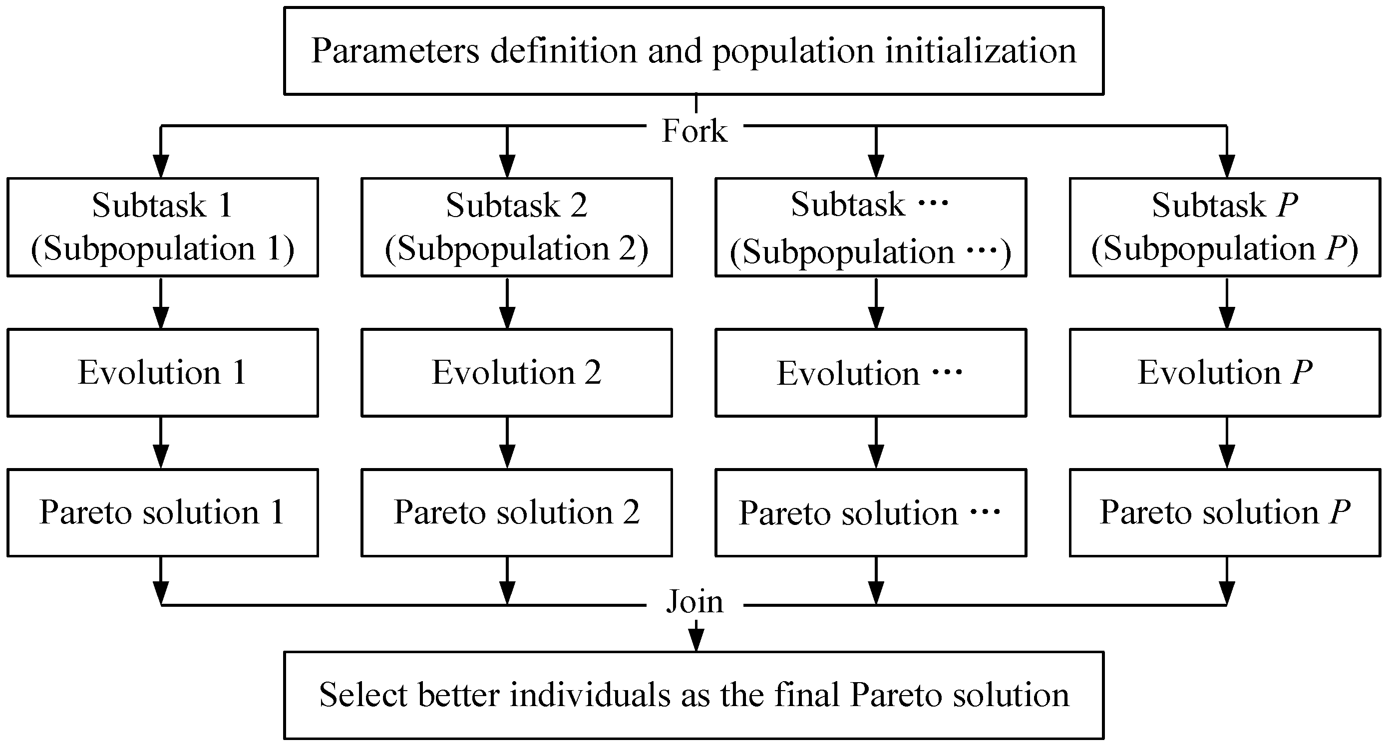
Preparation. Set the computing parameters, such as the population size, the maximum iteration and the worker threads for parallelization.

Step 2:

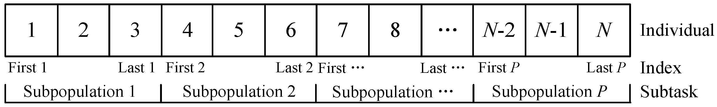
Initialization. Use the method in Section 4.2 to initialize all the individuals randomly in the problem space. Then, the main thread creates a thread pool and divides the whole population into several subpopulations to be concurrently optimized.

Step 3:

Subpopulation evolution. For any one subpopulation, use the corresponding crossover, mutation and selection operators to generate the members for the next cycle, and the whole iterative process will not be stopped until the maximum iteration is reached. To be mentioned, for the target subpopulation, the constraint handling method in Section 4.3 is used to repair infeasible solutions, while the method in Section 4.4 is employed to verify the performance of solutions.

Step 4:

Stop the calculation. The main thread will shut down the thread pool when all the subpopulations finish the calculation. Meanwhile, the results of each subpopulation are collected to form up the optimal Pareto solution set that will be exported as the final solutions for the problem.

5. Case Study

5.1. Description of the Power System

In this section, we choose a classical interconnected hydrothermal power system to verify the performance of the proposed method. Figure 5 shows a schematic map of the test hydrothermal system that has four cascaded hydro plants and three thermal plants. The scheduling period is one day, while the time interval is 1 h, and the whole number of scheduling intervals is 24. For the power system, the related coefficients data and operation limits of plants, system load at each period and hydraulic connection of reservoirs are taken from [32]. These data are not given here due to the space limitations. For testifying the feasibility of the proposed method, three different case studies were implemented in the following sections. For three cases, there is some difference in the calculation of the economic objective and transmission line losses, while they all have 168 decision variables and are subjected to the necessary boundary constraints, about 192 inequality constraints and 128 equality constraints. In addition, given that evolutionary algorithms use random numbers, there may be some difference in the optimal solutions found in different trails. Hence, to compare the performance of algorithms in each study, we run our algorithms 10 times with a different random number seed.

5.2. Parameters Setting

Based on lots of trials, the basic parameters of PMOGA are set as follows: the population size is 1200, the max iterations are 1000, and the size of external archive set is 30. The MOGA parameters are the same as that of PMOGA. Moreover, the number of worker threads in PMOGA is set to be equal to the number of computer cores. All the examples are encoded in Java language and executed on a personal computer with the Windows XP operating system and one Intel Xeon CPU [email protected] GHz (four cores).

5.3. Simulation Results

5.3.1. Case Study 1

In the first case study, for the sake of simplicity, the valve-point effect and transmission line losses are not considered. The result of multi-objective cultural algorithm based on particle swarm optimization (MOCA-PSO) is employed to testify the effectiveness of the proposed method [12]. In order to verify its stability and effectiveness, the algorithm runs the experiment 10 trials independently for each case with different initial populations. The best compromise solutions in 10 trails obtained by PMOGA are drawn in Figure 6, where it can be seen that both the fuel cost and emission have a small range of variation, and the 7th trial with smaller objectives is selected as the best one among the 10 trials [42]. In a similar way, the best trial for the following two cases can be obtained, which details are not given to save space.

Figure 7 shows the Pareto optimal front obtained by various methods, while

Table 1. The non-dominated schemes obtained by different methods for Case 1.

No.	MOGA		PMOGA		No.	MOGA		PMOGA
	fceo ($)	femi (lb)	fceo ($)	femi (lb)		fceo ($)	femi (lb)	fceo ($)	femi (lb)
1	39,716	17,913	39,687	17,936	16	39,812	16,385	39,782	16,136
2	39,721	17,858	39,689	17,528	17	39,821	16,317	39,795	16,074
3	39,722	17,718	39,692	17,381	18	39,833	16,214	39,806	16,023
4	39,728	17,581	39,695	17,235	19	39,854	16,150	39,818	15,977
5	39,730	17,444	39,697	17,144	20	39,866	16,100	39,830	15,937
6	39,732	17,328	39,701	17,049	21	39,879	16,057	39,851	15,879
7	39,736	17,208	39,705	16,951	22	39,894	16,022	39,871	15,836
8	39,744	17,094	39,713	16,795	23	39,910	15,980	39,891	15,804
9	39,751	17,007	39,717	16,720	24	39,922	15,958	39,908	15,781
10	39,755	16,908	39,723	16,644	25	39,947	15,930	39,924	15,763
11	39,761	16,751	39,728	16,573	26	39,972	15,907	39,950	15,740
12	39,772	16,696	39,734	16,508	27	39,989	15,891	39,971	15,727
13	39,777	16,604	39,746	16,388	28	40,002	15,878	40,000	15,714
14	39,790	16,531	39,758	16,291	29	40,026	15,866	40,020	15,709
15	39,797	16,434	39,770	16,207	30	40,048	15,863	40,048	15,706

lists the detailed objective values of both MOGA and PMOGA. To demonstrate the validity of the constraint handling strategy, Scheme 15 in Table 1 is selected as the trade-off scheduling plan, the hourly reservoir storage volume is drawn in Figure 8, while the water discharge rates of hydro plants and power outputs of all plants are shown in

Table 2. The detailed results of scheme 15 by PMOGA for case 1.

Period	Hydro Plant Output (MW)				Thermal Output (MW)
	Ph1	Ph2	Ph3	Ph4	Ps1	Ps2	Ps3
1	79.74	49.00	28.22	132.08	137.57	174.74	148.65
2	80.67	50.16	32.44	129.25	145.79	185.32	156.36
3	77.94	51.30	30.59	125.93	120.42	155.98	137.84
4	75.29	52.93	31.10	121.83	107.25	137.79	123.81
5	74.89	54.50	36.56	115.97	114.75	144.26	129.08
6	76.26	55.50	41.19	139.45	143.29	185.80	158.51
7	77.79	59.85	43.49	190.84	175.00	220.65	182.38
8	77.32	62.78	42.39	227.43	175.00	233.97	191.12
9	79.84	66.47	41.32	261.25	175.00	253.94	212.18
10	78.46	66.80	41.15	273.48	175.00	242.62	202.49
11	79.52	69.59	41.07	281.05	175.00	247.46	206.32
12	82.19	74.65	39.47	284.88	175.00	270.30	223.50
13	81.58	73.37	37.34	287.07	175.00	249.64	205.99
14	79.10	70.85	36.55	285.96	168.91	212.20	176.43
15	78.31	72.09	37.22	285.22	161.63	202.26	173.27
16	80.36	75.54	39.13	289.24	175.00	218.23	182.50
17	79.18	75.99	44.43	294.38	167.18	211.43	177.41
18	81.11	80.40	46.95	297.40	175.00	240.75	198.38
19	78.32	78.78	48.70	299.58	171.02	214.82	178.79
20	76.26	78.72	51.52	304.24	161.85	206.06	171.34
21	70.15	76.77	53.06	303.97	120.55	152.14	133.36
22	65.88	79.19	55.35	300.67	104.03	133.69	121.19
23	68.23	81.78	57.14	296.21	97.42	129.31	119.91
24	67.68	80.86	58.30	291.23	88.22	108.93	104.77

.

From the distribution of Pareto solutions in Figure 7, it can be clearly seen that the optimal PMOGA scheme dominates the solutions of other methods, which means that the PMOGA outperforms both MOGA and MOCA-PSO in terms of solution convergence and diversity. The economic objective and emission objective are in conflict with each other because the increasing value of one object will decrease the other one, which is in line with the results of [10,42]. That’s to say, for the SEEHTS problem, the lowest fuel costs may lead to damage of the environmental benefit. Meanwhile, with the same level of fuel cost, the proposed method can obtain the scheme with smaller emission cost in comparison with other methods. Moreover, Table 2 and Figure 8 indicate that the water discharge and storage volumes, power outputs are all in the predefined boundaries of the predefined operational constraints, demonstrating the feasibility and validity of the constraints handling method proposed in this research. Therefore, the proposed method can provide abundant technical options for planners and decision makers.

5.3.2. Case Study 2

In this section, the valve-point effect and the constraints of the first case are considered in the problem formulation. To compare the performance of the proposed method, the improved multi-objective gravitational search algorithm (IMOGSA) [13] and multi-objective differential evolution with adaptive Cauchy mutation (MODE-ACM) [4] are employed to solve the same problem. The Pareto optimal fronts by various methods are drawn in Figure 9, while the numerical results of MOGA and PMOGA are listed in

Table 3. The non-dominated schemes obtained by different methods for Case 2.

No.	MOGA		PMOGA		No.	MOGA		PMOGA
	fceo ($)	femi (lb)	fceo ($)	femi (lb)		fceo ($)	femi (lb)	fceo ($)	femi (lb)
1	43,497	16,864	41,630	17,338	16	45,162	16,195	44,282	16,133
2	43,509	16,805	41,634	17,331	17	45,330	16,152	44,440	16,111
3	43,608	16,743	41,770	17,222	18	45,555	16,112	44,745	16,071
4	43,710	16,697	41,771	16,854	19	45,777	16,073	45,018	16,038
5	43,726	16,648	41,954	16,759	20	46,023	16,043	45,257	16,010
6	43,853	16,597	42,140	16,686	21	46,160	16,007	45,647	15,965
7	43,923	16,552	42,330	16,617	22	46,374	15,990	45,940	15,932
8	44,018	16,488	42,506	16,556	23	46,510	15,978	46,197	15,906
9	44,140	16,429	42,690	16,501	24	46,747	15,958	46,592	15,867
10	44,263	16,366	42,821	16,448	25	46,983	15,906	46,848	15,845
11	44,379	16,324	43,035	16,366	26	47,269	15,901	47,088	15,830
12	44,469	16,287	43,168	16,327	27	47,631	15,879	47,382	15,806
13	44,649	16,269	43,321	16,291	28	47,883	15,860	47,682	15,787
14	44,777	16,245	43,665	16,230	29	48,216	15,855	47,978	15,777
15	44,929	16,223	44,000	16,180	30	48,418	15,844	48,318	15,771

. Moreover, the detailed operational processes of Scheme 15 in Table 3 are given in

Table 4. The detailed results of scheme 15 by PMOGA for case 2.

Period	Hydro Plant Output (MW)				Thermal Output (MW)
	Ph1	Ph2	Ph3	Ph4	Ps1	Ps2	Ps3
1	75.49	49.00	28.37	131.88	116.90	209.01	139.35
2	70.71	50.16	23.02	129.03	175.00	192.61	139.47
3	70.35	51.30	18.95	125.74	173.88	125.25	134.53
4	70.04	52.93	24.01	121.63	118.46	124.96	137.97
5	53.36	54.50	24.12	115.87	166.18	125.02	130.95
6	59.85	55.50	36.49	131.91	172.32	204.90	139.02
7	89.98	66.07	38.84	215.74	175.00	213.78	150.59
8	88.24	67.94	37.45	253.73	175.00	214.42	173.22
9	88.37	69.47	34.20	274.74	175.00	220.74	227.47
10	85.20	68.07	34.11	286.53	175.00	212.64	218.45
11	86.22	70.36	33.76	282.50	175.00	222.98	229.18
12	86.81	70.42	29.25	282.04	175.00	280.77	225.71
13	85.83	73.62	32.10	287.88	175.00	226.63	228.93
14	87.93	74.10	32.79	288.16	175.00	217.46	154.57
15	84.82	72.63	37.36	290.14	175.00	209.95	140.11
16	86.17	77.60	40.92	299.86	175.00	213.41	167.03
17	86.12	78.72	44.07	294.99	175.00	214.01	157.09
18	84.74	78.86	46.01	299.35	175.00	282.07	153.97
19	86.29	78.48	47.31	304.91	175.00	215.11	162.91
20	84.61	75.94	49.28	302.47	175.00	212.07	150.63
21	53.64	59.35	53.27	293.40	119.69	190.91	139.74
22	55.60	72.60	55.94	295.47	112.73	128.00	139.66
23	54.31	70.59	58.13	291.98	114.08	124.95	135.97
24	55.10	67.50	58.96	286.87	110.22	124.89	96.46

and Figure 10, respectively.

From Table 3 and Figure 9, it can be found that the proposed method can gives a group of solutions closer to the true optimal Pareto front compared with other evolution techniques, which proves that PMOGA can be an effective approach to solve complex multi-objective problems. Meanwhile, the results again prove that there is irreconcilable contradiction between the economic objective and the environmental objective. For example, in the best economic scheme, the fuel cost of PMOGA is reduced by 1867 ($) compared to the MOGA. In addition, the results in Table 4 and Figure 10 indicate that all the variables can satisfy the preset maximum and minimum constraints of the SEEHTS problem, which proves the validity of the proposed algorithm to deal with complicated constraints. Hence, from the above analysis, it can be concluded that PMOGA is an alternative method to handle the hydrothermal system scheduling problem.

Moreover, to further show the effectiveness of the proposed technique, its results is compared to the results of other methods in

Table 5. Comparison of solutions by PMOGA and other methods for case 2. ELS: economic load scheduling; EES: economic emission scheduling; CEES: combined economic emission scheduling; DE: differential evolution; QPSO-DM: quantum-behaved particle swarm optimization with differential mutation; and IQPSO: improved quantum-behaved particle swarm optimization.

Case	Method	Fuel Cost ($)		Emission (lb)
		Value	Improvement	Value	Improvement
ELS	PMOGA	41,630	-	17,338	-
	DE	43,500	1870	21,092	No comparison required
	QPSO-DM	41,909	279	30,724	No comparison required
	IQPSO	42,359	729	31,298	No comparison required
EES	PMOGA	48,318	-	15,771	-
	DE	51,449	No comparison required	18,257	2486
	QPSO-DM	45,392	No comparison required	17,659	1888
	IQPSO	45,271	No comparison required	17,767	1996
CEES	PMOGA	44,000	-	16,180	-
	DE	44,914	914	19,615	3435
	QPSO-DM	43,507	−493	18,183	2003
	IQPSO	44,259	259	18,229	2049

, including differential evolution (DE) [43], quantum-behaved particle swarm optimization with differential mutation (QPSO-DM) [44], and improved quantum-behaved particle swarm optimization (IQPSO) [1]. For the ELS case, the fuel cost is the only objective to be optimized, and it is not necessary to compare the emissions. Similarly, for the EES case, the emissions are the objective we care about, thus the fuel cost is not compared. From Table 5, it can be clearly observed that compared with methods reported in previous literatures, PMOGA provides results with fewer fuel cost and pollutant emissions in different cases. From the comparison with DE, QPSO-DM and IQPSO, the proposed algorithm can reduce the total fuel cost by 1870 ($), 279 ($) and 729 ($) in the ELS case; while the emission obtained by PMOGA is reduced by 2486 (lb), 1888 (lb) and 1996 (lb) in the EES case. In the CEES case, PMOGA can reduce simultaneously the fuel cost and emission compared with the DE and IQPSO, while its solution is not dominated by that of QPSO-DM. Thus, PMOGA is able to provide better solutions in comparison with other methods while satisfying all the constraints of the hydrothermal system.

5.3.3. Case Study 3

In this case, all constraints are considered for accurate formulation. Compared with previous cases, the power balance constraint makes it much more difficult to solve the SEEHTS because the power transmission losses changes dynamically with the outputs of plants in system. To verify its effectiveness, PMOGA is employed for the practical power system with MOGA and HMOCA [45]. The Pareto optimal schemes obtained by various methods are drawn in Figure 11, and the detailed objectives of PMOGA and MOGA are listed in

Table 6. The non-dominated schemes obtained by different methods for Case 3.

No.	MOGA		PMOGA		No.	MOGA		PMOGA
	fceo ($)	femi (lb)	fceo ($)	femi (lb)		fceo ($)	femi (lb)	fceo ($)	femi (lb)
1	43,891	17,984	42,687	18,471	16	45,567	17,250	44,624	17,292
2	43,898	17,920	42,713	18,440	17	45,733	17,216	44,914	17,223
3	43,948	17,858	42,895	18,339	18	45,940	17,181	45,190	17,173
4	44,046	17,808	42,897	18,099	19	46,188	17,148	45,470	17,134
5	44,151	17,748	43,018	18,002	20	46,381	17,094	45,737	17,094
6	44,276	17,715	43,166	17,907	21	46,599	17,069	45,949	17,062
7	44,377	17,666	43,323	17,830	22	46,778	17,038	46,159	17,032
8	44,449	17,609	43,485	17,760	23	47,054	16,986	46,520	16,980
9	44,546	17,560	43,665	17,693	24	47,355	16,953	46,799	16,944
10	44,635	17,511	43,794	17,627	25	47,589	16,924	47,193	16,898
11	44,790	17,487	43,909	17,563	26	47,868	16,883	47,470	16,869
12	44,925	17,443	43,976	17,495	27	48,149	16,868	47,840	16,834
13	45,040	17,403	44,169	17,403	28	48,445	16,832	48,146	16,814
14	45,266	17,357	44,299	17,364	29	48,770	16,828	48,502	16,798
15	45,470	17,304	44,452	17,326	30	49,047	16,804	48,969	16,783

. In addition, the 15th scheme is selected as the compromise plan, and its scheduling processes are given in

Table 7. The detailed results of Scheme 15 by PMOGA for Case 3.

Period	Hydro Plant Output (MW)				Thermal Output (MW)			Total (MW)	Loss PL (MW)	Load PD (MW)
	Ph1	Ph2	Ph3	Ph4	Ps1	Ps2	Ps3
1	74.00	49.00	25.90	132.38	127.53	210.05	139.80	758.66	8.66	750
2	66.21	50.16	21.49	129.41	175.00	209.78	139.67	791.72	11.72	780
3	74.18	51.73	23.78	126.15	169.25	126.76	137.90	709.75	9.75	700
4	71.95	52.90	34.20	123.33	108.56	126.02	139.44	656.40	6.40	650
5	53.37	54.47	23.28	116.27	102.52	189.88	137.11	676.90	6.90	670
6	61.81	55.47	37.93	132.47	175.00	209.94	139.04	811.66	11.66	800
7	92.14	67.06	41.85	228.93	175.00	210.76	146.52	962.26	12.26	950
8	83.06	64.83	38.43	229.43	175.00	210.63	224.37	1025.75	15.75	1010
9	86.24	62.39	35.80	259.95	175.00	275.29	211.98	1106.64	16.64	1090
10	87.15	72.84	34.17	286.49	175.00	292.70	146.06	1094.41	14.41	1080
11	88.90	73.67	34.76	276.11	175.00	294.93	172.02	1115.39	15.39	1100
12	83.42	70.04	35.67	282.33	175.00	294.31	227.28	1168.05	18.05	1150
13	86.24	67.30	32.08	287.40	175.00	250.75	228.35	1127.12	17.12	1110
14	88.40	73.81	36.53	291.57	175.00	234.43	143.28	1043.02	13.02	1030
15	87.67	74.79	38.86	290.33	175.00	214.74	141.13	1022.53	12.53	1010
16	82.46	75.17	41.48	288.84	175.00	269.66	141.07	1073.68	13.68	1060
17	90.76	79.65	44.94	297.15	175.00	231.20	144.34	1063.04	13.04	1050
18	83.99	80.42	47.46	301.07	175.00	292.90	153.94	1134.77	14.77	1120
19	85.04	81.06	48.67	303.87	175.00	247.51	142.20	1083.35	13.35	1070
20	80.56	78.56	49.66	301.51	175.00	212.09	166.04	1063.42	13.42	1050
21	53.76	67.10	54.18	288.62	104.96	209.72	139.85	918.20	8.20	910
22	54.05	61.35	56.38	293.95	104.08	160.19	137.43	867.42	7.42	860
23	61.03	75.11	57.88	292.64	105.76	125.29	139.51	857.22	7.22	850
24	56.77	74.17	58.71	286.47	103.00	125.21	101.68	806.01	6.01	800

and Figure 12, respectively.

From the results listed in Figure 11, it can be seen that, with the same size of external archive set, the Pareto optimal front distribution of PMOGA is wilder than other methods. Therefore, PMOGA has better performance than other methods in the solution diversity because its schemes are closer to the true Pareto optimal front. Moreover, from the data in Table 6, we can find that PMOGA can obtain schemes with smaller objective values than that of the traditional MOGA algorithm. For example, compared to MOGA, PMOGA can reduce the emission cost by 487 (lb) in the optimal economic scheme and decrease the fuel cost by 78 ($) in the optimal emission scheme, respectively. From Table 7 and Figure 12, we can find that the results of PMOGA can satisfy all kinds of equality and inequality constraints in the hydrothermal system at each period. Moreover, due to the valve-point and power transmission losses, compared with the compromise solution (Scheme 15) in previous case studies, there is some visible difference in the scheduling process of plants, and the fuel cost and emission cost are higher. Hence, PMOGA is an effective optimization algorithm for solving multi-objective problems.

5.4. Parallelization Performance

5.4.1. Metrics

The speedup and efficiency are two indicators frequently used to evaluate the performance of parallel computation [20,26], which are defined as follows:

$$S_P=T_S/T_P$$

(24)

$$E_P=S_P/P$$

(25)

where S_P and E_P are the speedup and efficiency, respectively; P is the number of cores; T_S is the serial computation time of the task in a single core; and T_P is the parallel computation time of the task with P computing units.

5.4.2. Results Analysis and Discussion

In this section, a group of scenarios with different populations and worker threads for three cases was executed to test the computational efficiency of parallel algorithms in multi-core environment.

Table 8. Serial and parallel computation time in different cases (time: s).

Scenario	Popsize	MOGA Time	PMOGA Time			PMOGA Speedup			PMOGA Efficiency
			2	4	8	2	4	8	2	4	8
Case 1	600	155.3	62.9	37.8	59.2	2.47	4.11	2.62	1.24	1.03	0.33
	800	244.7	94.8	53.7	78.5	2.58	4.56	3.12	1.29	1.14	0.39
	1000	346.7	127.0	68.9	95.8	2.73	5.03	3.62	1.36	1.26	0.45
	1200	455.5	163.6	80.9	120.0	2.78	5.63	3.79	1.39	1.41	0.47
Case 2	600	170.2	69.8	39.5	56.1	2.44	4.31	3.04	1.22	1.08	0.38
	800	258.0	97.5	54.4	79.0	2.65	4.74	3.27	1.32	1.18	0.41
	1000	349.1	131.5	66.0	102.9	2.65	5.29	3.39	1.33	1.32	0.42
	1200	461.6	167.2	82.3	121.1	2.76	5.61	3.81	1.38	1.40	0.48
Case 3	600	201.2	83.9	46.2	55.0	2.40	4.36	3.66	1.20	1.09	0.46
	800	288.1	116.3	63.0	75.2	2.48	4.57	3.83	1.24	1.14	0.48
	1000	393.7	151.9	80.4	88.1	2.59	4.90	4.47	1.30	1.22	0.56
	1200	508.0	192.2	95.5	106.6	2.64	5.32	4.77	1.32	1.33	0.60

lists the computation time in different scenario using both serial and parallel algorithms with various working threads.

From Table 8, it can be observed that the number of threads has no effect on the performance of algorithms in the serial situation, which means that conventional serial algorithm cannot make full use of the abundant computing resources available in a multi-core environment. On one hand, as the problem complexity increases, the MOGA execution time shows an obvious increase: with the same 600 individuals, the time consumption increases by 46 s from Case 1 to Case 3. On the other hand, the computation time of MOGA was increased rapidly with the increase of population: in the first case, the time for 1200 individuals increases 3-fold in comparison with 600 individuals. Thus, the MOGA will experience a rapid increase with the expansion of problem scale, which motivates us to develop a parallel algorithm to improve the performance of MOGA.

The time of PMOGA in different cases are also listed in Table 8. Compared with the MOGA, the PMOGA can significantly shorten the computation time. When there are 1200 individuals, the time reductions are 291.8 s, 374.5 s and 335.4 s for two threads, four threads and eight threads in the first case. In addition, the speedup increases with the number of individuals and threads, and there is super linear speedup when the number of worker threads is lesser than the maximum number of computational cores. This is because MOGA exhibits a quadratic growth in the computational complexity, which means that the population with greater size needs longer computation time; while in PMOGA, each subpopulation has relative smaller scale than MOGA, which dramatically reduces the time spent on iteration process of the algorithm. Besides, the speedup has a quick decrease when the number of worker threads exceeds the maximum number of computational cores. The reason lies in that under such circumstances, the thread pool needs more communication time and memory usage, which has a negative effect on the computational efficiency [21,26]. Thus, unreasonable worker threads only use some of the parallel resources in the multi-core computer, and the number of threads equal to the cores can obtain the best performance for most tasks.

Moreover, it can be seen from Table 8 that the efficiency in the same case has a quick drop as the computing units increase. This is because more time is spent on the internal storage sharing and working tasks communication between different computing units [20]. In other word, the task with larger scale tends to obtain greater efficiency in the same condition. Hence, the above analysis indicates that, for the SEEHTS problem, the parallel technology can make full use of the abundant computational resources to enhance the efficiency of algorithms.

6. Conclusions

The SEEHTS is classified as a multi-objective optimization problem subject to a set of complex constraints. In the present study, a new method known as PMOGA is proposed to handle the SEEHTS problem. Based on the Fork/Join parallel framework and natural parallelism of evolutionary algorithms, PMOGA makes full use of the abundant computational resources in a multi-core environment to enhance the performance of MOGA. A mature hydrothermal test system is used to test the effectiveness of the proposed approach. The simulation results in different cases indicate that compared with MOGA and several methods reported in the previous literature, PMOGA can obtain better results with less fuel cost and environment pollution. Besides, with two worker threads, the execution time of PMOGA for different population sizes is less than half that of MOGA for computing, demonstrating the effectiveness of the parallel technique. Furthermore, the speedup and efficiency of PMOGA are improved significantly with the expansion of problem scale, proving its potential to solve large-scale multi-objective optimization problems. Thus, the practicality and feasibility of PMOGA is verified adequately by the results of various cases, which indicate that the PMOGA can be a competitive tool for the SEEHTS problem. Since the choices of objective have great influence on the operational process, it is recommended that decision makers should pay careful attention to the hydrothermal scheduling so as to balance the economic and environmental objectives, and choose the approximate compromise scheme based on the actual demands of power systems.

References

1. Sun, C.; Lu, S. Short-term combined economic emission hydrothermal scheduling using improved quantum-behaved particle swarm optimization. Expert Syst. Appl. 2010, 37, 4232–4241. [Google Scholar] [CrossRef]
2. Guo, S.; Chen, J.; Li, Y.; Liu, P.; Li, T. Joint operation of the Multi-Reservoir system of the three gorges and the qingjiang cascade reservoirs. Energies 2011, 4, 1036–1050. [Google Scholar] [CrossRef]
3. Liu, P.; Nguyen, T.D.; Cai, X.; Jiang, X. Finding multiple optimal solutions to optimal load distribution problem in hydropower plant. Energies 2012, 5, 1413–1432. [Google Scholar] [CrossRef]
4. Qin, H.; Zhou, J.; Lu, Y.; Wang, Y.; Zhang, Y. Multi-objective differential evolution with adaptive Cauchy mutation for short-term multi-objective optimal hydro-thermal scheduling. Energy Convers. Manag. 2010, 51, 788–794. [Google Scholar] [CrossRef]
5. Lu, S.; Sun, C. Quadratic approximation based differential evolution with valuable trade off approach for bi-objective short-term hydrothermal scheduling. Expert Syst. Appl. 2011, 38, 13950–13960. [Google Scholar] [CrossRef]
6. Pan, L.; Guo, Z.; Liu, P.; Ma, L.; Li, Z. Comparison and analysis of macro energy scenarios in china and a decomposition-based approach to quantifying the impacts of economic and social development. Energies 2013, 6, 3444–3465. [Google Scholar] [CrossRef]
7. Ahmadi, A.; Sharafi Masouleh, M.; Janghorbani, M.; Yadollahi Ghasemi Manjili, N.; Sharaf, A.M.; Esmaeel Nezhad, A. Short term multi-objective hydrothermal scheduling. Electr. Power Syst. Res. 2015, 121, 357–367. [Google Scholar] [CrossRef]
8. Norouzi, M.R.; Ahmadi, A.; Sharaf, A.M.; Esmaeel Nezhad, A. Short-term environmental/economic hydrothermal scheduling. Electr. Power Syst. Res. 2014, 116, 117–127. [Google Scholar] [CrossRef]
9. Nezhad, A.E.; Javadi, M.S.; Rahimi, E. Applying augmented ɛ-constraint approach and lexicographic optimization to solve multi-objective hydrothermal generation scheduling considering the impacts of pumped-storage units. Int. J. Electr. Power Energy Syst. 2014, 55, 195–204. [Google Scholar] [CrossRef]
10. Zhang, H.; Zhou, J.; Fang, N.; Zhang, R.; Zhang, Y. Daily hydrothermal scheduling with economic emission using simulated annealing technique based multi-objective cultural differential evolution approach. Energy 2013, 50, 24–37. [Google Scholar] [CrossRef]
11. Immanuel Selvakumar, A. Civilized swarm optimization for multiobjective short-term hydrothermal scheduling. Int. J. Electr. Power Energy Syst. 2013, 51, 178–189. [Google Scholar] [CrossRef]
12. Zhang, R.; Zhou, J.; Wang, Y. Multi-objective optimization of hydrothermal energy system considering economic and environmental aspects. Int. J. Electr. Power Energy Syst. 2012, 42, 384–395. [Google Scholar] [CrossRef]
13. Li, C.; Zhou, J.; Lu, P.; Wang, C. Short-term economic environmental hydrothermal scheduling using improved multi-objective gravitational search algorithm. Energy Convers. Manag. 2015, 89, 127–136. [Google Scholar] [CrossRef]
14. Li, Y.; He, H.; Wang, Y.; Xu, X.; Jiao, L. An improved multiobjective estimation of distribution algorithm for environmental economic dispatch of hydrothermal power systems. Appl. Soft Comput. 2015, 28, 559–568. [Google Scholar] [CrossRef]
15. Pandit, M.; Srivastava, L.; Sharma, M. Environmental economic dispatch in multi-area power system employing improved differential evolution with fuzzy selection. Appl. Soft Comput. 2015, 28, 498–510. [Google Scholar] [CrossRef]
16. Xu, B.; Zhong, P.A.; Wan, X.; Zhang, W.; Chen, X. Dynamic feasible region genetic algorithm for optimal operation of a multi-reservoir system. Energies 2012, 5, 2894–2910. [Google Scholar] [CrossRef]
17. Basu, M. Economic environmental dispatch of fixed head hydrothermal power systems using nondominated sorting genetic algorithm-II. Appl. Soft Comput. 2011, 11, 3046–3055. [Google Scholar] [CrossRef]
18. Zhang, J.; Tang, Q.; Chen, Y.; Lin, S. A hybrid particle swarm optimization with small population size to solve the optimal short-term hydro-thermal unit commitment problem. Energy 2016, 109, 765–780. [Google Scholar] [CrossRef]
19. Shen, J.; Cheng, C.; Zhang, J.; Lu, J. Peak operation of cascaded hydropower plants serving multiple provinces. Energies 2015, 8, 11295–11314. [Google Scholar] [CrossRef]
20. Cheng, C.; Wang, S.; Chau, K.; Wu, X. Parallel discrete differential dynamic programming for multireservoir operation. Environ. Model. Softw. 2014, 57, 152–164. [Google Scholar] [CrossRef]
21. Li, X.; Wei, J.; Li, T.; Wang, G.; Yeh, W.W.G. A parallel dynamic programming algorithm for multi-reservoir system optimization. Adv. Water Resour. 2014, 67, 1–15. [Google Scholar] [CrossRef]
22. Li, M.; Xia, T.; Zhu, C.; Xi, B.; Jia, X.; Wei, Z.; Zhu, J. Effect of short-time hydrothermal pretreatment of kitchen waste on biohydrogen production: Fluorescence spectroscopy coupled with parallel factor analysis. Bioresour. Technol. 2014, 172, 382–390. [Google Scholar] [CrossRef] [PubMed]
23. Dias, B.H.; Tomim, M.A.; Marcato, A.L.M.; Ramos, T.P.; Brandi, R.B.S.; Junior, I.C.D.S.; João, A.P.S. Parallel computing applied to the stochastic dynamic programming for long term operation planning of hydrothermal power systems. Eur. J. Oper. Res. 2013, 229, 212–222. [Google Scholar] [CrossRef]
24. Aldinucci, M.; Danelutto, M.; Teti, P. An advanced environment supporting structured parallel programming in Java. Future Gener. Comput. Syst. 2003, 19, 611–626. [Google Scholar] [CrossRef]
25. Zhang, Y.; Jiang, Z.; Ji, C.; Sun, P. Contrastive analysis of three parallel modes in multi-dimensional dynamic programming and its application in cascade reservoirs operation. J. Hydrol. 2015, 529, 22–34. [Google Scholar] [CrossRef]
26. Zhang, Z.; Zhang, S.; Wang, Y.; Jiang, Y.; Wang, H. Use of parallel deterministic dynamic programming and hierarchical adaptive genetic algorithm for reservoir operation optimization. Comput. Ind. Eng. 2013, 65, 310–321. [Google Scholar] [CrossRef]
27. Tosun, U. On the performance of parallel hybrid algorithms for the solution of the quadratic assignment problem. Eng. Appl. Artif. Intel. 2015, 39, 267–278. [Google Scholar] [CrossRef]
28. Qiu, D.; Li, B.; Leung, H. Understanding the API usage in Java. Inf. Softw. Technol. 2016, 73, 81–100. [Google Scholar] [CrossRef]
29. Yuan, X.; Tian, H.; Yuan, Y.; Huang, Y.; Ikram, R.M. An extended NSGA-III for solution multi-objective hydro-thermal-wind scheduling considering wind power cost. Energy Convers. Manag. 2015, 96, 568–578. [Google Scholar] [CrossRef]
30. Deb, K.; Pratap, A.; Agarwal, S.; Meyarivan, T. A fast and elitist multiobjective genetic algorithm: NSGA-II. IEEE Trans. Evol. Comput. 2002, 6, 182–197. [Google Scholar] [CrossRef]
31. Wong, J.Y.Q.; Sharma, S.; Rangaiah, G.P. Design of shell-and-tube heat exchangers for multiple objectives using elitist non-dominated sorting genetic algorithm with termination criteria. Appl. Therm. Eng. 2016, 93, 888–899. [Google Scholar] [CrossRef]
32. Basu, M. An interactive fuzzy satisfying method based on evolutionary programming technique for multiobjective short-term hydrothermal scheduling. Electr. Power Syst. Res. 2004, 69, 277–285. [Google Scholar] [CrossRef]
33. Zhou, J.; Liao, X.; Ouyang, S.; Zhang, R.; Zhang, Y. Multi-objective artificial bee colony algorithm for short-term scheduling of hydrothermal system. Int. J. Electr. Power Energy Syst. 2014, 55, 542–553. [Google Scholar] [CrossRef]
34. Mandal, K.K.; Basu, M.; Chakraborty, N. Particle swarm optimization technique based short-term hydrothermal scheduling. Appl. Soft Comput. 2008, 8, 1392–1399. [Google Scholar] [CrossRef]
35. Rangaiah, G.; Sharma, S.; Sreepathi, B.K. Multi-objective optimization for the design and operation of energy efficient chemical processes and power generation. Curr. Opin. Chem. Eng. 2015, 10, 49–62. [Google Scholar] [CrossRef]
36. Pinto, F.S.; Figueira, J.R.; Marques, R.C. A multi-objective approach with soft constraints for water supply and wastewater coverage improvements. Eur. J. Oper. Res. 2015, 246, 609–618. [Google Scholar] [CrossRef]
37. Pinto, F.S.; Marques, R.C. Tariff suitability framework for water supply services: Establishing a regulatory tool linking multiple stakeholders’ objectives. Water Resour. Manag. 2016, 30, 2037–2053. [Google Scholar] [CrossRef]
38. Fang, L.; Qin, S.; Xu, G.; Li, T.; Zhu, K. Simultaneous optimization for hybrid electric vehicle parameters based on Multi-Objective genetic algorithms. Energies 2011, 4, 532–544. [Google Scholar] [CrossRef]
39. Li, F.F.; Qiu, J. Multi-Objective reservoir optimization balancing energy generation and firm power. Energies 2015, 8, 6962–6976. [Google Scholar] [CrossRef]
40. Qiu, W.; Zhang, J.; Yu, X.; Tang, Q. A small-population based binary PSO approach for unit commitment problem. J. Inf. Comput. Sci. 2015, 12, 3599–3610. [Google Scholar] [CrossRef]
41. Zhang, J.; Wang, J.; Yue, C. Small population-based particle swarm optimization for short-term hydrothermal scheduling. IEEE Trans. Power Syst. 2012, 27, 142–152. [Google Scholar] [CrossRef]
42. Tian, H.; Yuan, X.; Ji, B.; Chen, Z. Multi-objective optimization of short-term hydrothermal scheduling using non-dominated sorting gravitational search algorithm with chaotic mutation. Energy Convers. Manag. 2014, 81, 504–519. [Google Scholar] [CrossRef]
43. Mandal, K.K.; Chakraborty, N. Short-term combined economic emission scheduling of hydrothermal power systems with cascaded reservoirs using differential evolution. Energy Convers Manag. 2009, 50, 97–104. [Google Scholar] [CrossRef]
44. Lu, S.; Sun, C.; Lu, Z. An improved quantum-behaved particle swarm optimization method for short-term combined economic emission hydrothermal scheduling. Energy Convers. Manag. 2010, 51, 561–571. [Google Scholar] [CrossRef]
45. Lu, Y.; Zhou, J.; Qin, H.; Wang, Y.; Zhang, Y. A hybrid multi-objective cultural algorithm for short-term environmental/economic hydrothermal scheduling. Energy Convers. Manag. 2011, 52, 2121–2134. [Google Scholar] [CrossRef]
Figure 1. Map of the divide-and-conquer strategy.
Energies 10 00163 g001
Figure 2. Map of the population decomposition in parallel multi-objective genetic algorithm (PMOGA).
Energies 10 00163 g002
Figure 3. Map of the PMOGA algorithm.
Energies 10 00163 g003
Figure 4. Maps of the evolution process of (1) MOGA and (2) PMOGA.
Energies 10 00163 g004
Figure 5. Schematic map of the test hydrothermal system.
Energies 10 00163 g005
Figure 6. Best compromise solutions obtained by PMOGA in 10 independent trials.
Energies 10 00163 g006
Figure 7. The optimal Pareto front by different algorithms for Case 1.
Energies 10 00163 g007
Figure 8. The water storage processes of Scheme 15 by PMOGA for Case 1.
Energies 10 00163 g008
Figure 9. The optimal Pareto front by different algorithms for Case 2.
Energies 10 00163 g009
Figure 10. The water storage processes of Scheme 15 by PMOGA for Case 2.
Energies 10 00163 g010
Figure 11. The optimal Pareto front by different algorithms for Case 3.
Energies 10 00163 g011
Figure 12. The water storage processes of Scheme 15 by PMOGA for Case 3.
Energies 10 00163 g012